A GPU-based coupled SPH-DEM method for particle-fluid flow with free surfaces

A GPU-based coupled SPH-DEM method for particle-

fl

uid

fl

ow with

free surfaces

Yi He

⁎

, Andrew E. Bayly

, Ali Hassanpour

, Frans Muller

, Ke Wu

, Dongmin Yang

School of Chemical and Process Engineering, University of Leeds, Leeds LS2 9JT, UK b_{School of Civil Engineering, University of Leeds, Leeds LS2 9JT, UK}

a b s t r a c t

a r t i c l e i n f o

Article history:

Received 11 April 2018

Received in revised form 8 July 2018 Accepted 14 July 2018

Available online 17 July 2018

Particle-fluidflows with free-surfaces are commonly encountered in many industrial processes, such as wet ball milling, slurry transport and mixing. Accurate prediction of particle behaviors in these systems is critical to estab-lish fundamental understandings of the processes, however the presence of the free-surface makes modelling them a challenge for most traditional, continuum, multi-phase methodologies. Coupling of smoothed particle hy-drodynamics and discrete element method (SPH-DEM) has the potential to be an effective numerical method to achieve this goal. However, practical application of this method remains challenging due to high computational demands. In this work, a general purposed SPH-DEM model that runs entirely on a Graphic Processing Unit (GPU) is developed to accelerate the simulation. Fluid-solid coupling is based on local averaging techniques and, to accelerate neighbor searching, a dual-grid searching approach is adapted to a GPU architecture to tackle the size difference in the searching area between SPH and DEM. Simulation results compare well with experimental results on dam-breaking of a free-surfaceflow and particle-fluidflow both qualitatively and quantitatively, confirming the validity of the developed model. More than 10 millionfluid particles can be simulated on a single GPU using double-precisionfloating point operations. A linear scalability of calculation time with the number of particles is obtained for both single-phase and two-phaseflows. Practical application of the developed model is demonstrated by simulations of an agitated tubular reactor and a rotating drum, showing its capability in han-dling complex engineering problems involving both free-surfaces and particle-fluid interactions.

© 2018 The Authors. Published by Elsevier B.V. This is an open access article under the CC BY-NC-ND license (http://creativecommons.org/licenses/by-nc-nd/4.0/). Keywords:

GPU

Smoothed particle hydrodynamics Discrete element method Fluid-particle interaction Free surfaceflow Solid-liquidflow

1. Introduction

Understanding particle behaviors in free-surfaceflows is crucial to many natural phenomena and industrial processes, such as debris flow [1], wet ball milling [2,3], slurry transport [4], mixing and separa-tion in chemical and mineral processing [5–7] and additive manufactur-ing [8]. Despite wide popularity, application of traditional grid-based methods, such as coupled computationalfluid dynamic (CFD) and dis-crete element method (DEM), to handle particles in free-surfaceflows is still challenging due to the presence of free-surfaces, especially splashing and fragmentations [9–11]. Additional detection algorithms are required to track the free surfaces for grid-based Eulerian methods, such as volume offluid [9], marker-and-cell [10] and level-set method [11]. In addition, numerical diffusion may arise due to advection terms. On the other hand, grid-based Lagrangian methods face prob-lems of mesh distortion, which requires expensive mesh re-generation. The presence of splashing and fragmentations requires a numerical method which can handle the discrete nature of the free-surface flows. SPH, as a meshless method, shows strong potentials in this regard

as it discretize thefluid into a set of particles, thus allowing the dynam-ics of the free-surfaceflows to be readily captured. Since the pioneer work of Gingold and Monaghan [12], SPH has been widely used to model free-surfaceflows in manyfields [13]. It has been recently extended to deal with solid particles in free-surfaceflows by coupling SPH with DEM [7,14–17]. Nevertheless, application of this method to engineering problems remains limited due to associated high computa-tional cost. This is especially the case when complex moving boundaries are present. Thus, a high performance implementation of the SPH-DEM method is necessary for applications in engineering practice.

Coupling of SPH and DEM enables a unified Lagrangian particle-based method, well suited for applications where free-surfaces and strongfluid-particle interactions coexist. Approaches for coupling the momentum transfer between thefluid and particles can be classified into two groups: resolved and unresolved methods. In the resolved method the SPH particles are significantly smaller than the solid parti-cles and theflow around the solid particles is explicitly resolved. In the unresolved method the SPH particles are of a comparable size of the solid particles and empirical force correlations are used to capture the momentum transport between phases. For resolved simulation, a variety of methods have been developed to enable no-slip conditions at solid surfaces. Potapov et al. [18] coupled SPH with DEM to simulate ⁎ Corresponding author.

E-mail address:[email protected](Y. He).

https://doi.org/10.1016/j.powtec.2018.07.043

0032-5910/© 2018 The Authors. Published by Elsevier B.V. This is an open access article under the CC BY-NC-ND license (http://creativecommons.org/licenses/by-nc-nd/4.0/).

Contents lists available atScienceDirect

Powder Technology

shearflow of neutrally buoyant particles, where no-slip boundary condition is enabled by placing SPH particles inside large solid particles [19]. Densities of the interior SPH particles are updated in the same manner as thefluid SPH particles while moving the interior SPH parti-cles with the solid partiparti-cles. This approach was verified with experi-mental results on the drag force and size of the wake for_fluid_flow around a circular cylinder. Canelas et al. [20] coupled SPH with a so-called distributed contact DEM, where the solid body is represented by a set of small particles withfixed relative position. The interaction betweenfluid and solid particles are calculated in a manner similar to the methodology of dynamic boundary conditions [21]. The interactions among solid bodies are calculated through the small constituent parti-cles by means of soft-sphere collision model. This model shows good comparison with experiments on tracking blocks subjected to a dam-break wave [20] and on a debrisflow [22]. Ren et al. [23] also reported a similar method to study stability of 2D blocks on a slope due to wave-structure interaction. Since the fluid resolution has to be sufficiently small to resolveflow structure around the particle, high computational demand is thus inevitable when dealing with a large number of solid particles. The requirement of a larger size of solid parti-cles than thefluid particles further limits their range of applicability, especially considering a wide size distribution of solid particles is com-monly encountered in practical systems.

On the other hand, phase interaction in the unresolved simulation is handled by empirical force correlations. Both one-way and two-way coupled SPH-DEM methods have been reported. For example, Komoroczi et al. [24] combined SPH with DEM by treating either DEM particles as SPH particles or treating SPH particles as DEM particles. Cleary et al. [4,5] treated the solid bed as a dynamic porous media by av-eraging the velocities and porosities of the DEM particles, through which the SPHfluid is able toflow. This one-way coupled method has been applied to predict slurry transport in SAG mills [4] and to model slurryflow on a double deck vibrating banana screen [5] in mineral processing. Sun et al. [6] reported a two-way coupled SPH-DEM method in which a boundary model based on variational approach is explicitly included in the momentum equation. A unified boundary representa-tion is enabled for both phases, eliminating the redundant wall particles for thefluid phase. Similarly, Robinson et al. [17] developed a coupled SPH-DEM method based on the locally averaged Navier-Stokes equa-tions. The model showed good agreement with sedimentation test cases with increasing complexity, namely, settling of single sphere, constant block of particles and multiple particles. The fully coupled SPH-DEM method is gaining popularity in different engineering applica-tions, including fluid-particle-structure interaction problem with free-surfaceflow [14,15] and landslide generated surge waves [16] and particle separation due to density difference in waste recycling [7]. To date, however, most of these studies are concerned with 2D sim-ulation [14–16] or limited to a very small scale [7,17], therefore, devel-oping a general SPH-DEM model capable of accelerating simulation is of great importance for practical problems in engineering applications.

Computational efficiency of numerical methods is closely related to the progress of hardware architecture. GPU-based parallelism has been increasingly applied to speedup simulations of particle-based nu-merical methods due to high memory bandwidth and instruction throughput offered by GPU processors, such as Molecular Dynamics [25,26], Lattice Boltzmann Method [27–29], SPH [30,31] and DEM [32–36]. GPU-based implementations show orders of magnitude faster than their serial counterparts, making it very attractive for schemes that can make use of the single instruction multiple data architecture. Due to the locality of particle interactions, both SPH and DEM schemes require identification of neighboring particles. In pure SPH models the interaction length is greater than twice the particle diameter, where in pure DEM simulations there is no long distance force and the interaction search area is approximately the solid particle diameter. In coupled SPH-DEM systems, the interactions between different particle types leads to increased complexity. To accelerate neighbor searching on

GPU, different algorithms have been reported, including thek-dtree method [37] and spatial subdivision approaches, such as the bounding volume hierarchy method [38,39] and the uniform grid method [35]. Thek-dtree structure needs to be reconstructed at every time step, thus not suitable for discrete methods while the spatial subdivision approaches are limited by the fact that the grid size needs to be large enough to host the largest particles. Application of these searching methods mentioned above to SPH-DEM is thus not straightforward, especially on a GPU platform. A general purpose SPH-DEM program also needs to be efficient at GPU memory management. To the best of our knowledge, coupling of SPH and DEM methods that run entirely on a GPU platform has yet to be reported.

Starting from the theoretical background, this work will address the development of a general purposed GPU-based SPH-DEM method in detail. A dual-grid searching approach is incorporated to handle the dif-ference in the particle interacting range between SPH and DEM. Model validation and performance analysis of the GPU-based model will be evaluated for both the single phase and the particle-fluidflows, respec-tively. Practical application of the GPU-based model to chemical engineering will be illustrated by the simulating free-surfaceflows in an agitated tubular reactor and particle-fluidflows in a rotating drum. The paper is organized as follows: the model formulation isfirst presented inSection 2followed by a detailed description of the GPU implementation, including the neighbor searching method, memory management and programflow. Then, the validation, engineering application and performance of the developed model in handling both single-phase flow and particle-fluid flow with free-surfaces are addressed separately inSection 3.

2. Model description and GPU implementation

To achieve unresolved simulation, different approaches to couple DEM to SPH have been reported [6,14–17], which are essentially solving governing equations of the conventional Two Fluid Model (TFM) [40] in the framework of SPH, which are given as,

∂ðερfÞ

∂t þ∇∙ðερfuÞ ¼0 ð1Þ

∂ðερfuÞ

∂t þ∇∙ðερfuuÞ ¼−∇P−Spþ∇∙ðετfÞ þερfg ð2Þ

withρfthefluid density,Ppressure acting on thefluid phases,τfthe viscous stress tensor andgthe acceleration due to gravity.εis the vol-ume fraction of_fluid in each cell.Spis the source term due to the rate of momentum exchange between thefluid phase and the solid phase. The coupling strategy adopted here is similar to that proposed by Robinson et al. [17]. In this section, an overview of the SPH and the DEM methods used to discretize the governing equations and the strategy of phase coupling are provided. A detailed description of the force models used in DEM can be found elsewhere [41–43]. For ease of reading, thefluid particles are labeled as particleaandbwhile the solid particles are labeled as particleiandj.

2.1. Fluid phase: SPH

The methodology behind SPH is based on the theory of integral interpolants, the interpolated value of a function A(r) at positionris expressed as,

Að Þ ¼r Z Að Þr0 Wðjr−r0j;hÞdr0 ð3Þ

associated properties, such as density, pressure and momentum. The fluid particles follow theflow due to pressure gradient, viscous shear and body force while acting as interpolation points for their neighbors. The integral interpolant at the position of the particle is approximated by,

Að Þ ¼ra X

b

Ab

mb

ρb

Wðj jrab;hÞ ð4Þ

withmbandρbthe mass and density of particleb, |rab| being the distance between twofluid particles. The summation is taken over all particles within the support domain of particlea.

The kernel functionW(|rab|,h)must obey a number of mathematic constraints, including positivity, monotonically decreasing, compact support and normalization. In this study, the Wendland kernel function is used since it can achieve a good balance between numerical accuracy and computational cost [44].

Wðj jrab;hÞ ¼αD 1−q

2

4

1þ2q

ð Þ0≤q≤2 ð5Þ

whereαDis 7/8πh3in 3D.q= |rab|/h. In practice, the kernel function vanishes when the particle separation is greater than 2hto achieve a compact support domain.

2.1.1. Continuity equation

Applying the SPH particle approximation, the continuity equation of Eq.(1)can be written as,

dρa dt ¼

X

b

mbvab∇aWabðj jrab;hÞ ð6Þ

with∇aW(|rab|,h) the gradient of the kernel function at the position of particlea, andvab=va−vbis the velocity vector.ρdenotes the super-ficialfluid density defined asρa¼ερf, withεthe volume fraction of fluid andρfthe intrinsicfluid density.

2.1.2. Equation of state

In the weakly compressible SPH schemes [45],fluid particles are driven by local pressure gradient. Pressure is expressed as a function of thefluid density, giving a quasi-incompressible equation of state as follows:

P¼B ρa ερ0

γ

−1

ð7Þ

withγ= 7 andρ0reference density of thefluid.Bis a pressure constant determines the speed of sound bycs2=γB/ρ0. The densityfluctuation in fluidflow is proportional toM2_{whereMis the Mach number. By} limiting the Mach number, theflow can be considered practically in-compressible. To limit the density variation within 1%, the coefficient Bcan be calculated as,

B¼100_γρ0v2

max ð8Þ

2.1.3. Momentum equation

The momentum equation of Eq.(2)in SPH form is given by,

dva dt ¼−

X b mb Pa ρ2 a þPb ρ2 b þRab " #

∇aWabðj jrab;hÞ þΠabþSaþg ð9Þ

withPthe pressure due tofluid phase,Πabthe viscosity term andRabthe term due to tensile instability andSathe couple term due to solid parti-cles. The symmetrical form of the pressure gradient term is taken in order to reduce error arising from particle inconsistence. The stress

termsΠabrepresenting the viscous diffusion derived by [19] is incorpo-rated into the momentum equation,

Πab¼X b

mbðμaþμbÞrab∙∇aWabðj jrab;hÞ

ρaρb r2 abþ0:01h

2

vab ð10Þ

whereμis the dynamic viscosity. In the weakly compressible SPH, tensile instability is often attributed as the cause of unphysical particle clumping. This phenomenon is especially significant in materials with an equation of state which can give rise to negative pressures, which reduces numerical accuracy due to the uneven particle distribution. To remove the instability, [46] introduced an additional pressure between particles to prevent particle from forming small clumps. This artificial pressure termRabis added to the momentum equation, given as,

Rab¼0:01 Pa ρ2 a

þPb ρ2 b

!

Wðj jrab;hÞ WðΔp;hÞ

4

ð11_Þ

whereΔpis the initial particle spacing.

2.1.4. Moving the particles

To keep an orderlyflow of particle, the particles are moved using the XSPH variant,

dra dt ¼va−ϵ

X

b mb

ρabvabWabðj jrab;hÞ ð12Þ

where _{ρab¼ ðρ}aþρbÞ=2 andϵ is a problem-dependent constant,

ranging from 0 to 1. It moves a particle at a velocity close to the average velocity of its neighbors. In this study,ϵis set to 0.3.

2.1.5. Boundary treatment

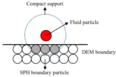
When a SPH particle approaches a rigid boundary, the support domain of its kernel will be truncated by the boundary. Ideally, the boundary treatment should compensate for the lack of particles beyond the boundary and provide enough repulsive force to prevent particles from penetration. Different treatments have been proposed to this end, including kernel re-normalization [47], ghost particles [48], layers offixedfluid particles, repulsive particles [45] and dynamic particles [49–51]. Sun et al. [6] introduced a correction to the SPH approximation where the boundary information are explicit included without using extra wall particles. Together with level-set functions, a unified bound-ary was enabled for both the solid phase and thefluid phase. In the pres-ent study, a generalized wall boundary treatmpres-ent that is capable of handling arbitrarily shaped geometries was adopted [52]. As shown in Fig. 1, solid wall is discretised into dummy particles whose properties do not evolve with time. These wall particles provide support for the kernel interpolants of thefluid particles. The pressure and velocity at the position of a wall particle is interpolated from surroundingfluid

DEM boundary

Fluid particle

Compact support

SPH boundary particle

particles to ensure a non-slip boundary condition of the solid walls, which are given by,

vw¼2va− X

b

vbWabðj jrab;hÞ

X

b

Wabðj jrab;hÞ ð13Þ

Pw¼

X

f

PfWwfðjrwfj;hÞ þðg−awÞX f

ρfrwfWwfðjrwfj;hÞ

X

f

Wwfðjrwfj;hÞ

ð14Þ

ρw¼ρ0

Pw

B þ1

1

γ

ð15Þ

withvathe prescribed wall velocity,awthe acceleration of the wall and | rwf| being the distance betweenfluid particle and wall particle. In prac-tice, however, wall penetration cannot be fully avoid where violent fluid-wall interactions exist. Therefore, in this study, the repulsive force proposed by Monaghan [45] is combined with the above boundary treatment to fully prevent wall penetration.

2.2. Solid phase: DEM

In DEM, the motion of solid particles is tracked by Newton’s second law of motion, written as,

mdv

dt¼FfþFcþmg ð16Þ

Idω

dt ¼TfþTc ð17Þ

wherem,I,vandωare, the mass, inertia, translational and rotational velocities of the element, respectively. The force and torques acting on each particle consists of several contributions, including the hydrody-namic components,FfandTf, arising fromfluid-particle interaction, the collision components,FcandTc, due to solid-solid interaction and mgthe gravity. The collisions between particles are handled by a soft-sphere model that allows for inter-particle overlap. The collision force includes the normal contact forceFn, normal damping forceFd,n, tangential contact forceFtand tangential damping forceFd, t. The normal contact is described by Hertz theory while tangential elastic frictional contact is based on Mindlin and Deresiewicz theory [53]. The normal and tangential contact forces are given as,

Fn_¼4 3E

_R1=2 δ3=2

n n^ ð18Þ

Ft¼−δtμtj jFn δt

j j 1− 1−

minj jδt;δt;max δt;max

3=2

" #

ð19Þ

in which theR∗,E∗andδt, maxare calculated as,

1 R¼

1 Riþ

1

Rj ð20Þ

1 E¼

1−ν2 i

Ei þ

1−ν2 j

Ej ð

21Þ

δt;max¼ 2−ν

ð Þ

2−2νμtδn ð22Þ

withRiandRjbeing the radius of two particles in contact.Eandνare the Young’s Modulus and Poisson’s ratio of solid particles, respectively.δn andδtrepresent the overlap in normal and tangential directions andμt is the sliding friction.

The equations used to calculate damping in normal and tangential directions are given by,

Fd_;n¼−cn 8mE

ffiffiffiffiffiffiffiffiffiffi

Rδn

p

1=2

vn ð20Þ

Fd_;t¼−ct 6μtmEj jFn

ffiffiffiffiffiffiffiffiffiffiffiffiffiffiffiffiffiffiffiffiffiffiffiffiffiffiffiffiffi

1−j jδt=δt;max

p

δt;max

!1=2

vt ð21Þ

wherecnandctare the normal and tangential damping coefficient, respectively. The normal damping coef_ficient can be directly linked to the restitution coefficientein the normal direction by,

cn¼−lne=

ffiffiffiffiffiffiffiffiffiffiffiffiffiffiffiffiffiffiffiffiffiffiffi

π2_{þ ln}2 e

q

ð23Þ

The normal restitution coefficienteis defined as the ratio of post-col-lisional contact velocity to pre-colpost-col-lisional contact velocity.

The collision torqueTcis composed of the torque due to the tangen-tial forceTtand the torqueTrdue to particle rolling friction resulting from the elastic hysteresis losses or viscous dissipation [54], calculated as,

Tt¼ FtþFd;t

R ð24Þ

Tr¼μrR_{j j}Fnω^n ð25Þ

where_μris the rolling friction andω^n¼ωn=jωnjwithωnthe angular

velocity.

2.3. Phase coupling

The local porosity at the position offluid particleais calculated by a summation over neighboring DEM particles within a coupling lengthhc,

given as,

εa¼1− X

j

Wajð ÞhcVj ð26Þ

withVjthe volume of DEM particlej,Waj(hc) the SPH kernel andhcthe

coupling length for the interaction between two phases. The coupling length should be larger than the diameter of solid particle but small enough to capture local feature of the porosityfield. Here, the coupling length is set to be same as the SPH smoothing length.

For the solid particles, forces due tofluidflow are modelled. The total fluid force can be split into a pressure gradient force and a drag force.

Fi¼−Við−∇Pþ∇∙τÞ þFd ð27Þ

withVithe particle volume,∇Pthe pressure gradient andFdthe drag force. The pressure gradient is evaluated at solid particleiusing a Shepard corrected SPH interpolation [55], given as,

−∇P_þ∇∙τ

ð Þi¼

1

X

b mb

ρbWabð Þhb

X

b mb

ρbθbWibð Þhb ð28Þ

θa¼−

X b mb Pa ρ2 a þPb ρ2 b !

∇aWabð Þ þhb Πab ð29Þ

Thefluid-particle drag forceFddepends on the local porosity and rel-ative velocity betweenfluid and particle. For the dense particlefluid flow, the drag model of Ergun and Wen & Yu [56,57] is used, which is based on experimental measurements.

withβthe interphase momentum exchange coefficient, which is given by,

β¼

150μð1−εÞ 2

εd2i

þ1::75ð1−εÞρf

di ju−vij ðε<0:8Þ 3

4CD εð1−εÞ

di ρfju−vijε

−2:65 _ðε>0:8Þ

8 > > > < > > > :

ð31Þ

whereCDis the drag coefficient. It can be calculated as,

CD¼

24 1:0þ0:15Re0:687 p

Rep Rep≤1000

0:44 Rep>1000

8 > < >

: ð32Þ

in which the particle Reynolds numberRepis defined asRep=ρdpε|u −vp|/μ.

The rate of momentum exchange in the right hand of Eq.(2)for each SPH particle is calculated by a weighted average offluid-particle coupling force acting on the surrounding DEM particles within the cou-pling lengthhc, so that Newton’s third law of motion is satisfied, which

is given by,

Sa¼−ma ρa

X

j

1

X

b mb

ρbWabð Þhb

FiWajð Þhc ð33Þ

2.4. GPU implementation

2.4.1. Neighbor searching

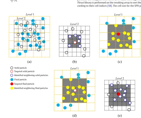
The locality of interaction in both SPH and DEM methods highlights the importance of an efficient neighbor searching algorithm. Neighbor searching is often regarded as the most time demanding aspect of a par-ticle-based method. Although extensive studies have been conducted to optimize the searching process, implementation of a searching algo-rithm on the GPU platform is still not straightforward for the coupled SPH-DEM method. The reason is attributed to the size difference be-tween the support domain, 2h, of the SPH particles and the diameter, d, of the DEM particles. DEM calculations are mainly concerned with particles in direct contact or with short-range interactions, whilst long-ranged interactions are present in the SPH calculations. If the size of the search grid is set as the smoothing length of the SPH particles, 2h, it would inevitably include redundant DEM particles. A dual-grid searching approach was therefore implemented to reduce the size of the search domain for the solid phase and thus accelerate the neighbor searching process.Fig. 2shows a schematic view of the dual-grid searching approach applied to a coupled system where particles of two phases are of the same size. The hollow circles represent the DEM particles while the solid circles represent the SPH particles. Based on a traditional linked-cell method, the implemented searching method consists of two steps: particle mapping and all-level searching.

Firstly, particles are mapped onto different grids according to their type: solid particles are mapped onto Level 1 while fluid particles are mapped ontoLevel 2. A radix sort algorithm from the Thrustlibrary is performed on the resulting array to sort the particles ac-cording to their cell indices [58]. The cell size for the SPH particles is set

(a)

(b)

(c)

(d)

(e)

Level

1

Level

2

Level

2

Level

1

Fluid particle Solid particle

Targeted solid particle

Identified neighboring solid particles

Targeted fluid particle

Identified neighboring fluid particles

Level

1

Level

2

as 2h+ΔSPHwhile it is set asdmax+ΔDEMfor the DEM particles, in whichdmaxis the maximum particle diameter. Consequently, only par-ticles in the neighboring cells contribute to the update of a same phase (Fig. 2(b) and2(c)). The searching area is shaded for illustration purposes inFig. 2. The purpose of introducing an extra searching gap Δis to avoid conducting the particle mapping and searching at every time step. A large value ofΔmeans more time are needed to conduct neighbor searching for each time. It is thus a balance between the fre-quency of searching and the time cost of each searching routine. Its value depends on factors like the particle velocities and solid concentra-tion, but normally smaller than the particle size. In this study, it is set as 0.3 times of the particle size. Potential neighbors are then identified by looping through all levels of the searching grid. For SPH particles, the fluid neighbors are detected fromLevel 2while its solid neighbors are searched onLevel 1. For the DEM particles, the contact detection between solid particles is conducted onLevel 1while the interaction withfluid particles is performed onLevel 2. For interactions between phases, the search area depends on the size ratio between the size of the SPH particle support domain and the DEM particle size. To_find neighboring DEM particles, the SPH particle is mapped intoLevel 1, as shown inFig. 2(e). In this illustrative example,⌈2h/d⌉= 3 (where the nomenclature⌈x⌉returns the smallest integer larger thanx). Searching is therefore conducted by looping through the three surrounding layers of the DEM cells. On the other hand, tofind neighboring SPH particles for a given DEM particle, searching is only performed within the sur-rounding SPH cells and the mapped cell itself as⌈d/2h⌉= 1, as shown inFig. 3(d).

2.4.2. Memory management

A unique feature of the DEM calculation is the need to record the contact status between two contacted particles. It is used to determine the friction status, either in static friction or in dynamic friction. If plastic deformation or inter-particle bonding is considered, a large amount of memory is required to keep the contact history information [43]. Additionally, double-precisionfloating point accuracy is required to minimize numerical errors. Consequently to enable the efficient solu-tion of large-scale problems, it is important to optimize the algorithm to balance memory consumption and computing efficiency. To this end, a neighbor list is only constructed for the DEM particles as each SPH particle can host a large amount of neighbors due to its large size of support domain. Instead, the step of particle mapping for the SPH par-ticles is conducted occasionally while the step of all-level searching is conducted at every time step. The reconstruction of DEM neighbor list and the particle mapping step for SPH particles are triggered when ac-cumulated displacement of any particles exceeds a specified threshold: ΔDEM/2 for DEM particles andΔSPH/2 for SPH particles, respectively.

In this study, both the neighbor list and associated contact history in-formation are saved in the global memory on the GPU. Each time step, neighbor searching and force calculations require frequent access to this data. The memory layout has therefore been optimized to boost the efficiency of data fetching. GPU threads are grouped into warps of 32 threads and each memory operation is issued per warp, meaning that one memory fetch can return a cache line of 128 bytes. Conse-quently to promote coalesced memory access, and therefore maximize the efficiency of each fetch, the neighbor index and contact history data arrays of each DEM particle are organized in a column-major pattern.

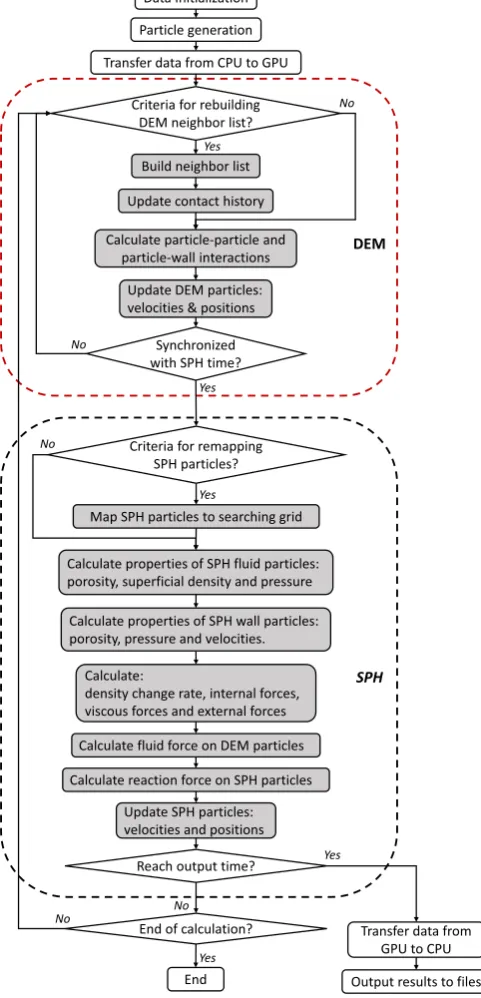
2.4.3. Programflow

The coupled SPH-DEM method was implemented using C++ and Compute Unified Device Architecture (CUDA) developed by NVIDIA. The GPU program was formulated using a single-program multiple-data (SPMD) technique, where the same program is executed by multi-ple threads simultaneously. Due to the discrete nature of the particle methods, GPU threads are assigned to each particle (either DEM or SPH particle). As a result, neighbor searching, force calculation and

time integration of the equation of motion can be carried out independently for each particle using different GPU kernel functions. For efficient use of the GPU memory, parameters that remain the same during simulation, such as material properties, are stored in the constant memory (a type of read-only memory on the GPU with fast data fetching) while other particle-related information, including posi-tions, velocities, forces and contact histories, are stored in the global memory on the GPU.

Fig. 3shows theflow chart of the algorithm that runs on a single GPU. The whole program can be divided into two major parts: DEM calculation and SPH calculation. For each type of calculation, there are three major components: i) neighbor searching (DEM) or particle mapping (SPH), ii) force computation and iii) time integration of the

Data Initialization

Update DEM particles: velocities & positions

Map SPH particles to searching grid

Calculate:

density change rate, internal forces, viscous forces and external forces

Calculate fluid force on DEM particles

Calculate reaction force on SPH particles

Update SPH particles: velocities and positions Calculate properties of SPH fluid particles: porosity, superficial density and pressure

DEM

Particle generation

Build neighbor list

Update contact history

Calculate particle-particle and particle-wall interactions

Synchronized with SPH time?

Calculate properties of SPH wall particles: porosity, pressure and velocities.

End of calculation? Transfer data from GPU to CPU Reach output time?

Output results to files End

Transfer data from CPU to GPU

Criteria for rebuilding DEM neighbor list?

Criteria for remapping SPH particles?

SPH

Yes No

Yes No

Yes

No No

Yes Yes

No

equation of motion using an explicit time integration method (forward Euler method). The time step for time integration in SPH is limited by the CFL-condition based on the arti_ficial sound speed and the maximum flow speed and viscous condition [13] while the time step used for DEM calculation is determined based on a Rayleigh wave propagation criteria [59].

The program starts by reading pre-defined initial positions and the associated properties of the SPH particles fromfiles generated from a pre-processing step. The solid particles are subsequently randomly generated and allowed to settle within the required region or the geom-etry. Once this initialization is complete the DEM and SPH calculations are started. During each step, the DEM calculation arefirst performed following an order of searching neighbors, updating contact histories, calculating forces and updating the particle velocities and positions. The DEM calculation iterates multiple times until the DEM time is syn-chronized with the SPH time. The SPH calculation is then started by mapping thefluid particles onto the searching grid, namely assigning thefluid particles into axially-aligned cells, ready for neighbor searching in the following steps. The porosity at the position of each_fluid particle is calculated from surrounding solid particles (Eq.(26)). The pressure of fluid particles is updated using the equation of state based on thefluid superficial density (Eq.(7)). Then, the interaction betweenfluid parti-cles is calculated by solving the continuity (Eq.(6)) and momentum equations (Eq.(9)). The phase coupling is achieved by calculating the fluid force acting on the solid particles (Eq.(27)) and then the reaction force on thefluid particles is calculated using a weighted-average of the forces from the solid particles (Eq.(33)). Finally, thefluid particles’ density, velocity and position are updated. These calculations are re-peated over the simulation time. It should be noted that the bandwidth between CPU and GPU limits the efficiency of memory transfer. Therefore, we only retrieve simulation data occasionally back to the CPU for data recording. With the exception of the data transfer all the calculations are performed on the GPU by means of issuing a set of CUDA kernel functions.

3. Results and discussion

In this section, validation, application and performance evaluation of the GPU-based models are carried out. The model validation is focused on the SPH model and the coupled SPH-DEM model as the GPU execution of the DEM model has been validated and applied in previous studies of powderflow and compaction [41–43]. Dam break simulations with single and two-phaseflow are chosen for this purpose due to their simplicity and wide acceptance as validation tests for free-surfaceflows. The validated models are then applied to two systems: a novel tubular reactor where thefluidflow is agitated by a perforated tube and a quasi-steady solid-liquidflow in a rotating cylindrical drum. These were selected to examine the capability of the models in handling complex systems encountered in engineering practice.

3.1. Single phaseflow

3.1.1. Model validation: single phase dam break

3.1.1.1. Validation and effect offluid resolution.

The single phase dam break system modelled here has been widely used for SPH method validation [6,7,14,16] by comparison with the ex-perimental results of Koshizuka et al. [60]. Thefluid particles are set up initially on a Cartesian lattice, as shown inFig. 4.

The predictedflow patterns were compared with those from the experiments at a series of time instants, as shown inFig. 5. Particles are colored by the velocity magnitude. A wedge-shaped water front is generated and moves rapidly towards the right after the sudden removal of the confinement (Fig. 5(a)). The water front starts to deflect and deform once hitting on the vertical wall, a significant amount of water is deflected vertically (Fig. 5(b)) and then falls back due to gravity,

generating a plunging surface wave which travels back towards the left side of the tank (Fig. 5(c) and (d)). Theflow patterns agree well with those observed experimentally, indicating that the present model is ca-pable of qualitatively capturing the_flow behavior in the dam-breaking. The effect of thefluid particle size on the predictedflow patterns was investigated by comparing the results form 2, 3 and 4 mm fluid particles. The overallflow patterns were very similar however more de-tailed structure was seen with smaller particles. This is illustrated in Fig. 6, which compares theflow patterns seen at 0.8 s. It can be seen that the size of the void formed under the leading front of the water wave increases with the smaller particle size.

A quantitative estimate of the model accuracy is made by comparing predicted and experimental propagation of the wave front before hitting the right side vertical wall. To this end, two dimensionless numbers are defined: the position of the leading wave frontx∗and the characteristic timet∗, which are given as,

x¼x=a ð30Þ

t¼tpffiffiffiffiffiffiffiffiffiffiffi2g=a ð31Þ

xis the position of the wave front in the horizontal direction;ais the width of the water column before collapsing;tis the physical time andgis gravitational acceleration. As shown inFig. 7, the SPH slightly underpredict the position of the leading front at the initial stage while a better agreement can be seen aftert∗> 1.5. The fair agreement of the results gives a difference within 5% of the predicted value, demon-strating that the model is able to provide accurate quantitative data for single phase free-surfaceflows.Fig. 7also shows the effect of particle resolution on the position of the wave front, with decreasing particle size, the wave front propagates slightly quicker, indicating that a better agreement can be reached when usingfiner particle resolution.

3.1.1.2. Performance evaluation.

The performance and scalability of the GPU-based SPH method were evaluated by increasing the dam width in the simulation above from 200 mm to 12,800 mm, while other dimensions remain the same. This increased the particle number to 14.142 million in the largest

simulation. The calculation time required for these simulations is shown inFig 8. A comparison of the same implementation run on two different Nvidia GPU cards, Tesla K80 and P100, is also shown. The mean calcula-tion time per iteracalcula-tion was found to scale linearly with the number of particles (R2_{> 0.99). It shows that more than 10 million particles can} be simulated on both cards. The performance of the P100 card is consis-tently better than that of the K80 card in both the procedures of particle mapping and a calculation cycle. The ratio of the scalability (de_fined as the slope of the linearfit) between K80 and P100 is 1.83 for the process of particle mapping and 3.19 for a calculation cycle. This is primarily be-cause the P100 card provides 1.6 times more GFLOPS (double precision) and 3 times more memory bandwidth than the K80 card.

3.1.2. Application of SPH: agitated tubular reactor

The validated model was applied to an agitated tubular reactor (ATR), a novel, intensified, reactor used for continuous chemical processing. The ATR system consists of a series of tubes with free-mov-ing internal agitators, which are mounted on a shakfree-mov-ing platform. The internal agitators have a cylindrical shape with caps attached to both ends to prevent direct contact with the tube surface, thus reducing mill-ing of the catalyst particles. Compared with conventional mechanically agitated reactors, such as stirred tank reactors, the ATR has no driving shafts and baffles. Instead, the lateral shaking of the system drives the agitator motion. The resulting radial mixing is independent on the axialflow rate. Theflexibility to independently control axialflow and

mixing make it well suited for handling slurries, gas/liquid mixture and catalysed reactions [62,63].

3.1.2.1. Flow system.

In the present study, a periodic section of a single external tube is subjected to a sinusoidal oscillation. The passive internal agitator that drives theflow is a perforated tube with ellipse-shaped surface holes. Fig. 9(a) shows a schematic view of the geometrical and particle repre-sentation of the modelled system in SPH.

The collision of the agitator with the external tube is modelled using an approach which is analogous to a soft-sphere collision model used in DEM calculations; the agitator is treated as a single element whose motion is tracked by Newton's second law of motion [64]. Factors deter-mining its motion include gravity and forces due to collision with the external tube. The contact between the agitator and the tube wall only occurs at the end caps, consequently the collision contact diameter is set as the cap size. For simplicity, however,fluid forces are not consid-ered in the present model due to the fact that the motion of the agitator is dominated by the collision between structures. The temporal velocity of the tube is described as a sinusoidal motion, given by,

U tð Þ ¼2πfAcos 2ð πftÞ ð32Þ

withfthe shaking frequency andAthe shaking amplitude. As a result, the computational domain is not stationary but constantly changing

with the shaking of the external tube, which would complicate the model implementation and data analysis. In order to enable a stationary domain, simulations are performed in the reference frame of the shak-ing tube. To this end, an acceleration is imposed to both the agitator and thefluid, given by,

a tð Þ ¼−4π2

f2Asin 2ð πftÞ ð33Þ

with a direction opposite to the shaking. Computationally, it is prohibi-tive to model the whole length of the reactor, a section of ATR system is thus modelled with periodic boundary condition applied in the axial direction. The workingfluid is water. Other modelling parameters are summarized inTable 1, which are typical operational parameters. A total physical time of 5s is simulated.

3.1.2.2. Motion of the agitator.

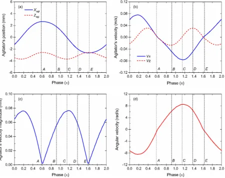
The agitator presents a well-behaved periodic motion due to the si-nusoidal oscillation of the reactor tube. The motion of the agitator quickly reaches a stable state after thefirst two periods. The behaviour of the agitator in a typical period are shown inFig. 10. From phase 0 to 0.5π, the reactor tube moves toward the right hand side with a de-creasing velocity, while the agitator accelerates towards the bottom of the tube followed by a deceleration when it moves upwards. The

Fig. 7.Comparison of the propagation of the wave front as a function of characteristic time between SPH results and experiments [61].

Fig. 8.Computational cost of a calculation cycle as a function of the number of particles on different GPU cards. The results are shown in the form of the wall clock time per simulated time step averaged over 1000 timesteps.

(a)

(b)

(c)

Agitator

End cap

Lateral shaking

Fluid Internal agitator

External tube

Fig. 9.(a) Schematic of the cross-section of the reactor tube in the Coflore ATR1 reactor (courtesy AM Technology), (b) Geometrical representation of the agitator and (c) particle representation of the simulated ATR system, in which the size of thefluid particle is 0.2 mm.

Table 1

Parameters used in simulation.

External tube

Amplitude,A(mm) 7.1

Frequency,f(Hz) 4.06

Diameter,D(mm) 25.4

Internal agitator

Inner diameter,Di(mm) 13.8

Outer diameter,Do(mm) 14.4

Density,ρs(kg/m3) 7800

Cap size,Scap(mm) 1.5

Moment of Inertia,I(kg·m2

) 2.516 × 10-7

Young’s modulus,E(Pa) 1.0 × 108

Poisson ratio,ν 0.3

Sliding friction coefficient,μt 0.3

Restitution coefficient,e 0.6

Fluid particles

Fluid density,ρf(kg/m3) 1000

agitator reaches the highest point around phaseAshortly after the tube reverses its moving direction at 0.5π. At this stage, the tube continues to move to the left hand side at an increasing speed while the agitator slides down towards the bottom at an increasing speed. The maximum velocity of the agitator is around 0.076 m/s which corresponds to 42% of the maximum shaking velocity (0.181 m/s). After the tube pass the mid-dle point of its moving region (>1.0π), the agitator reaches the bottom of the tube at phaseC. After that, the agitator start to move upward at a decreasing speed.

3.1.2.3. Agitatedflowfield.

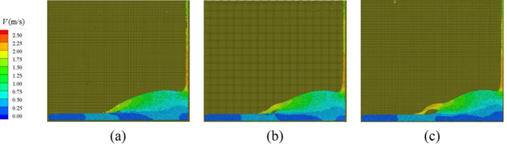
Fig. 11(b) shows the contours offluid velocity magnitude at thefive selected phases marked inFig. 10(a). Combining the information from Fig. 10(a)-(d), an illustration of the agitator’s motion and the position of the shaking tube in the global reference frame are given inFig. 11 (a). In general, the motion of thefluid is mainly driven by the shaking of the reactor tube as suggested by the rotation of thefluid as a whole. However, local variations can still be seen due to the presence of the ag-itator. For example, at phaseA, local maximum of thefluid particles are found located at the interstice between the agitator and the reactor, similar to that of the phaseE. This is primarily due to the small relative velocity between the agitator and the reactor tube at these phases. The fluid particles at the contact region are being squeezed out by the agita-tor. Due to the presence of the surface holes, a repeated pattern of the fluid velocity along the axial direction can be observed at the free sur-face. The complex dynamics captured in the ATR system shows the strong potential of applying the developed GPU-based SPH in

understanding and further optimizing the design and the operational conditions of chemical reactors where the free-surfaceflows present.

3.2. Particle-_fluid_flow

3.2.1. Model validation: two-phase dam break

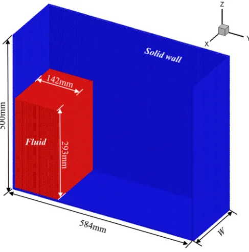
To validate the coupling between SPH and DEM, a two-phase dam break is simulated and is compared with the experimental re-sults reported by Sun et al. [6]. This test case has also been adopted to validate coupled SPH-DEM approaches in other studies [7,15]. The water tank has overall dimensions: 200 mm × 150 mm × 150 mm, and is split into two volumes by a movable gate 50 mm from one end. Water with a depth of 100 mm along with a packed particle bed are blocked by the gate. The dam break is initiated by moving the gate upward at a constant speed of 0.68 m/s. The initial particle configuration of the SPH-DEM simulation is shown inFig. 12.

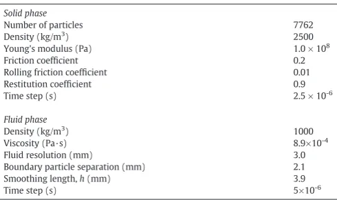
For the solid phase, a total mass of 200 g spherical particles arefirst randomly generated behind the moving gate. Then, they are allowed to settle under gravity until the total kinetic energy essentially vanishes. For thefluid phase, SPH particles with material properties of water are orderly distributed behind the gate. Other modelling parameter can be found inTable 2.

Fig. 13compares the simulation with the experiments at a time in-terval of 0.5 s. The SPH particles are colored by volume fraction while the DEM particles are colored by the velocity magnitude. The dam break is initiated by moving the gate upward at a constant velocity of 0.68 m/s. With restriction of the vertical gate, particles are driven by

thefluid drag to move along with theflow direction. In comparison, both thefluid and the solid phase observed in experiments are well reproduced, indicating qualitatively comparable simulation results. The minimumfluid volume fraction produced by the simulation is around 0.33 which is close to the packing fraction of random loose packing (0.64). In the simulation, however, the wave front of the water lags the experiment very slightly, this can be seen inFig. 13d; in the experiment the water has reached the left hand wall, where as in the simulation the water wave has not quite made impact.

Quantitative comparisons of the extent of propagation of the leading front of both thefluid and the solid phases are shown inFig. 14. The same dimensionless numbers are used as the previous single phase case. It can be seen that the simulation matches well with the experi-ments. Discrepancies, however, are seen at initial stage of the dam break for thefluid phase (0.015 s to 0.035 s) and at the later stage for

the solid phase (>0.14 s). Several factors may contribute to the discrep-ancy, including the use of uncalibrated DEM parameters, such as the friction coefficient and the restitution coefficient, as also noted by Markauskas et al. [7], and the lack of the lubrication mechanism in the present simulation which would also lead to an underestimation of the position of the solid front.

3.2.2. Application of coupled SPH-DEM: rotating drum

In mineral and chemical processing, rotating drums are often used for mixing or grinding. Water is added to suppress dust or to modify the operational conditions, leading to a typical slurry_flow. In this section, the GPU-based coupling method is applied to model the parti-cle-fluidflow in a rotating cylindrical drum. The setup is the same as reported in the work of Sun et al. [6]. The predicted results arefirst com-pared with experiments in terms of the bed shape and dimensions.

Fig. 11.Velocity profile in a half-filled ATR system at different phases, in which phaseA= 0.581π,B= 0.906π,C= 1.150π,D= 1.393πandE= 1.637π. Fluid particles are colored by velocity magnitude in the reference frame of the tube.

Fig. 12.Particle configuration of the two-phase dam break test case for SPH-DEM, solid particles are not shown. Fluid particles are colored by volume of fraction.

Table 2

Modelling parameters used in the simulation.

Solid phase

Number of particles 7762

Density (kg/m3

) 2500

Young's modulus (Pa) 1.0 × 108

Friction coefficient 0.2

Rolling friction coefficient 0.01

Restitution coefficient 0.9

Time step (s) 2.5 × 10-6

Fluid phase

Density (kg/m3

) 1000

Viscosity (Pa·s) 8.9×10-4

Fluid resolution (mm) 3.0

Boundary particle separation (mm) 2.1

Smoothing length,h(mm) 3.9

Then, the performance of the GPU implementation is evaluated by scaling up the device.

3.2.2.1. Model validation.

In this study, the diameter and the length of the drum are both 100 mm. The drum rotates at a constant speed of 104 rpm, with half of it filled with water. A quasi-steady state of the solid particle bed is reached at this speed. In the simulation, a total of 7755 solid particles with a di-ameter of 2.7 mm are used, replicating the simulation reported by Sun et al. [6]. The rest of the parameters are the same as summarized in Table 2.Fig. 15(a) shows the initial configuration of the SPH particles. A single layer of wall particles are used. The randomly generated solid particles are allowed to settle down in the drum without the in_fluence offluid force to form a packed bed. Then the drum starts to rotate. After reaching a steady state, a particle bed with bilinear slope is ob-served. As shown inFig. 15(b) and (c), the present simulation is capable of qualitatively reproducing the bilinear slope close to that observed in the experiment.

Quantitative comparisons are made of both the average height and the width of the bed. The dimensions are obtained by averaging over 50 equally spaced sample times over a period of 10 s. The comparisons with experimental results are given inTable 3, together with a compar-ison to the simulation results of Sun et al. [6]. The present simulation

accurately captured the width of the bed, with a difference smaller than 1%. However, the height of the bed is slightly under-predicted with a difference around 8% compared to the experiment. Compared to the simulation of Sun et al. [6], the difference is about 4.8%. This dis-crepancy seems to arise from differences in contact models and no proper calibration of the parameters. For example, we used the Hertz model for the normal contact force and the Mindlin and Deresiewicz theory for the tangential elastic frictional contact while [6] used a spring-dashpot model.

3.2.2.2. Performance evaluation.

The rotating drum is scaled to evaluate the performance of the coupled SPH-DEM on the Tesla P100 card. Four different diameters of the drum, 100 mm, 200 mm, 300 mm and 400 mm, are tested. The length of the drum is the same as its diameter in all cases. The water and article volume fractions were kept constant across all simulations. The computational time cost for the DEM calculations and the SPH cal-culations were recorded and are shown inFig. 16. The elapsed time per step is calculated by averaging over 10,000 steps. It can be seen that the time cost of the SPH part is consistently more than an order of magnitude higher than that of the DEM part. Moreover, the computa-tional cost for both parts increase linearly with increasing number of particles.

4. Conclusion

A GPU-based program has been developed to accelerate the simula-tions of single phase_fluid_flow and particle-_fluid_flow involving free-surfaces, with the goal of an efficient technique for application to multi-phase chemical processes. The free-surfacefluidflow is resolved using SPH, while DEM is adopted to track the motion of solid particles if present, thus a unified particle-based modelling framework was established. The coupling between the two phases is achieved using local averaging techniques. A dual-grid neighbor searching method was proposed to handle coupling between phases, due to the difference

Fig. 14.Normalized leading front as a function of scaled time: comparison between simulation and experiments [6].

Fig. 15.(a) Particle representation of the simulated rotating drum, in which the size of thefluid particle is 3 mm and the typical snapshot of (b) experiment [6] and (b) the present simulation, in which the solid particles are represented by yellow spheres while thefluid particles are represented by blue cubes. The bilinear slope is indicated by the red lines in thefigure.

Table 3

Comparison of the bed dimensions between simulation and results of Sun et al. [6]. Bed dimensions (standard

deviation)

Experiment [6]

Simulation of [6]

Current study

Width, mm 73.41 (1.25) 71.45 (0.79) 73.78 (0.708)

in the size of influencing area between solid particles andfluid particles. The algorithm and the memory management was specifically designed to suit the GPU platform.

For the single phaseflow, a single-phase dam breakflow was simu-lated to validate the SPH model. The model accuracy was evaluated in terms of theflow pattern and evolution of the position of the wave front, all showed good agreement with published experimental results. A sensitivity test indicates more detailedflow structure can be obtained usingfinerfluid particle resolution. The performance of the SPH algo-rithm implemented on GPU was evaluated by changing the width of the dam. A linear scalability was obtained between the averaged calcu-lation time per step and the number of particles. The overall perfor-mance achieved on the Tesla P100 card was about 2 times faster than that on the Tesla K80 card. The model’s ability to predict free-surface flows in complex engineering problems was demonstrated by a novel tubular reactor with a free-moving perforated agitator.

For particle-fluidflow, validation was conducted on a similar exam-ple case, this time with particles present. A good agreement with exper-imental results was obtained for the temporal evolution of both the solid particle bed and thefluid wave front. A typical application to chemical process was demonstrated by a simulation of a quasi-steady particle-fluid flow in a rotating drum. The obtained results have shown satisfactory predictions in terms of bed shape and bed

dimensions. The performance of the coupled SPH-DEM model was eval-uated by scaling up the size of the rotating drum. The SPH related calcu-lations consumed more time than those of the DEM. The computational time for both the DEM and the SPH particle scales linearly with the par-ticle number.

With the reliable results and acceptable scalability obtained from the GPU platform, the coupled SPH-DEM model has demonstrated its po-tential to contribute to an improved understanding of the practical problems encountered in chemical processing. Future work on extend-ing the implementation to multiple GPUs by means of Message Passextend-ing Interface is on course to further enhance the computational capabilities.

Acknowledgments

The authors would like to thank the European Commission for supporting this work as part of the research project "Intensi_fied by De-sign® for the intensification of processes involving solids handling" un-der the H2020 SPIRE programme (SPIRE-08-2015-680565). This work was undertaken on ARC3, part of the high performance computing facil-ities at the University of Leeds, UK.

Reference

[1] K. Hutter, B. Svendsen, D. Rickenmann, Debrisflow modeling: a review, Continuum. Mech Therm. 8 (1996) 1–35.

[2] C. Tangsathitkulchai, Acceleration of particle breakage rates in wet batch ball mill-ing, Powder Technol. 124 (2002) 67–75.

[3] M. Hussain, Y. Oku, A. Nakahira, K. Niihara, Effects of wet ball-milling on particle dis-persion and mechanical properties of particulate epoxy composites, Mater. Lett. 26 (1996) 177–184.

[4] P.W. Cleary, M. Sinnott, R. Morrison, Prediction of slurry transport in SAG mills using SPHfluidflow in a dynamic DEM based porous media, Miner. Eng. 19 (2006) 1517–1527.

[5] J.W. Fernandez, P.W. Cleary, M.D. Sinnott, R.D. Morrison, Using SPH one-way coupled to DEM to model wet industrial banana screens, Miner. Eng. 24 (2011) 741–753.

[6] X. Sun, M. Sakai, Y. Yamada, Three-dimensional simulation of a solid-liquidflow by the DEM-SPH method, J. Comput. Phys. 248 (2013) 147–176.

[7] D. Markauskas, H. Kruggel-Emden, V. Scherer, Numerical analysis of wet plastic par-ticle separation using a coupled DEM-SPH method, Powder Technol. 325 (2018) 218–227.

[8] X. Wang, M. Jiang, Z.W. Zhou, J.H. Gou, D. Hui, 3D printing of polymer matrix com-posites: a review and prospective, Compos. Part B-Eng. 110 (2017) 442–458.

[9] C.W. Hirt, B.D. Nichols, Volume offluid (Vof) method for the dynamics of free boundaries, J. Comput. Phys. 39 (1981) 201–225.

[10] M.F. Tome, L. Grossi, A. Castelo, J.A. Cuminato, N. Mangiavacchi, V.G. Ferreira, F.S. de Sousa, S. McKee, A numerical method for solving three-dimensional generalized Newtonian free surfaceflows, J. Non-Newton Fluid. 123 (2004) 85–103.

[11]S. Osher, J.A. Sethian, Fronts propagating with curvaturedependent speed -algorithms based on Hamilton-Jacobi formulations, J. Comput. Phys. 79 (1988) 12–49.

[12] R.A. Gingold, J.J. Monaghan, Smoothed particle hydrodynamics - theory and applica-tion to non-spherical stars, Mon. Not. R. Astron. Soc. 181 (1977) 375–389.

[13] J.J. Monaghan, Smoothed particle hydrodynamics and its diverse applications, Annu. Rev. Fluid Mech. 44 (2012) 323–346.

[14] K. Wu, D.M. Yang, N. Wright, A coupled SPH-DEM model forfluid-structure interac-tion problems with free-surfaceflow and structural failure, Comput. Struct. 177 (2016) 141–161.

[15] K. Wu, D. Yang, N. Wright, A. Khan, An integrated particle model forfluid–particle–

structure interaction problems with free-surfaceflow and structural failure, J. Fluids Struct. 76 (2018) 166–184.

[16] H. Tan, S.H. Chen, A hybrid DEM-SPH model for deformable landslide and its gener-ated surge waves, Adv. Water Resour. 108 (2017) 256–276.

[17] M. Robinson, M. Ramaioli, S. Luding, Fluid-particleflow simulations using two-way-coupled mesoscale SPH-DEM and validation, Int. J. Multiphase Flow 59 (2014) 121–134.

[18]A.V. Potapov, M.L. Hunt, C.S. Campbell, Liquid-solidflows using smoothed particle hydrodynamics and the discrete element method, Powder Technol. 116 (2001) 204–213.

[19]J.P. Morris, P.J. Fox, Y. Zhu, Modeling low Reynolds number incompressibleflows using SPH, J. Comput. Phys. 136 (1997) 214–226.

[20] R.B. Canelas, A.J.C. Crespo, J.M. Dominguez, R.M.L. Ferreira, M. Gomez-Gesteira, SPH-DCDEM model for arbitrary geometries in free surface solid-fluidflows, Comput. Phys. Commun. 202 (2016) 131–140.

[21] A.J.C. Crespo, M. Gomez-Gesteira, R.A. Dalrymple, Boundary conditions generated by dynamic particles in SPH methods, Comput. Mater. Con. 5 (2007) 173–184.

[22] R.B. Canelas, J.M. Dominguez, A.J.C. Crespo, M. Gomez-Gesteira, R.M.L. Ferreira, Re-solved Simulation of a Granular-Fluid Flow with a Coupled SPH-DCDEM Model, J. Hydraul. Eng. 143 (2017).

[23] B. Ren, Z. Jin, R. Gao, Y.X. Wang, Z.L. Xu, SPH-DEM modeling of the hydraulic stability of 2D blocks on a slope, J. Waterw. Port. Coast (2014) 140.

[24] A. Komoroczi, S. Abe, J.L. Urai, Meshless numerical modeling of brittle-viscous defor-mation:first results on boudinage and hydrofracturing using a coupling of discrete element method (DEM) and smoothed particle hydrodynamics (SPH), Comput. Geosci. 17 (2013) 373–390.

[25] J.A. Anderson, C.D. Lorenz, A. Travesset, General purpose molecular dynamics simu-lations fully implemented on graphics processing units, J. Comput. Phys. 227 (2008) 5342–5359.

[26] W.M. Brown, P. Wang, S.J. Plimpton, A.N. Tharrington, Implementing molecular dy-namics on hybrid high performance computers - short range forces, Comput. Phys. Commun. 182 (2011) 898–911.

[27] F. Kuznik, C. Obrecht, G. Rusaouen, J.J. Roux, LBM basedflow simulation using GPU computing processor, Comput. Math. Appl. 59 (2010) 2380–2392.

[28] M. Januszewski, M. Kostur, Sailfish: aflexible multi-GPU implementation of the lat-tice Boltzmann method, Comput. Phys. Commun. 185 (2014) 2350–2368.

[29]C. Obrecht, F. Kuznik, B. Tourancheau, J.J. Roux, Multi-GPU implementation of the lattice Boltzmann method, Comput. Math. Appl. 65 (2013) 252–261.

[30]J.M. Dominguez, A.J.C. Crespo, D. Valdez-Balderas, B.D. Rogers, M. Gomez-Gesteira, New multi-GPU implementation for smoothed particle hydrodynamics on hetero-geneous clusters, Comput. Phys. Commun. 184 (2013) 1848–1860.

[31]Q.G. Xiong, B. Li, J. Xu, GPU-accelerated adaptive particle splitting and merging in SPH, Comput. Phys. Commun. 184 (2013) 1701–1707.

[32] J. Xu, H.B. Qi, X.J. Fang, L.Q. Lu, W. Ge, X.W. Wang, M. Xu, F.G. Chen, X.F. He, J.H. Li, Quasi-real-time simulation of rotating drum using discrete element method with parallel GPU computing, Particuology 9 (2011) 446–450.

[33]N. Govender, D.N. Wilke, S. Kok, Blaze-DEMGPU: modular high performance DEM framework for the GPU architecture, SoftwareX 5 (2016) 62–66.

[34] J.Q. Gan, Z.Y. Zhou, A.B. Yu, A GPU-based DEM approach for modelling of particulate systems, Powder Technol. 301 (2016) 1172–1182.

[35]J.W. Zheng, X.H. An, M.S. Huang, GPU-based parallel algorithm for particle contact detection and its application in self-compacting concreteflow simulations, Comput. Struct. 112 (2012) 193–204.

[36]Y. He, T.J. Evans, A.B. Yu, R.Y. Yang, A GPU-based DEM for modelling large scale powder compaction with wide size distributions, Powder Technol. 333 (2018) 219–228.

[37]K. Zhou, Q.M. Hou, R. Wang, B.N. Guo, Real-time KD-tree construction on graphics hardware, Acm T Graphic. (2008) 27.

[38]C. Lauterbach, Q. Mo, D. Manocha, gProximity: hierarchical GPU-based operations for collision and distance queries, Comput. Graph. Forum 29 (2010) 419–428.

[39] S. Pabst, A. Koch, W. Strasser, Fast and scalable CPU/GPU collision detection for rigid and deformable surfaces, Comput. Graph. Forum 29 (2010) 1605–1612.

[40]T.B. Anderson, R. Jackson, A. Fluid Mechanical, Description offluidized beds, Ind. Eng. Chem. Fundam. 6 (1967) 527.

[41] Y. He, T.J. Evans, Y.S. Shen, A.B. Yu, R.Y. Yang, Discrete modelling of the compaction of non-spherical particles using a multi-sphere approach, Miner. Eng. 117 (2018) 108–116.

[42] Y. He, T.J. Evans, A.B. Yu, R.Y. Yang, DEM investigation of the role of friction in mechanical response of powder compact, Powder Technol. 319 (2017) 183–190.

[43] Y. He, Z. Wang, T.J. Evans, A.B. Yu, R.Y. Yang, DEM study of the mechanical strength of iron ore compacts, Int. J. Miner. Process. 142 (2015) 73–81.

[44]W. Dehnen, H. Aly, Improving convergence in smoothed particle hydrodynamics simulations without pairing instability, Mon. Not. R. Astron. Soc. 425 (2012) 1068–1082.

[45] J.J. Monaghan, Simulating free-surfaceflows with SPH, J. Comput. Phys. 110 (1994) 399–406.

[46] J.J. Monaghan, SPH without a tensile instability, J. Comput. Phys. 159 (2000) 290–311.

[47] J.K. Chen, J.E. Beraun, T.C. Carney, A corrective smoothed particle method for bound-ary value problems in heat conduction, Int. J. Numer. Methods Eng. 46 (1999) 231–252.

[48]P.W. Randles, L.D. Libersky, Smoothed particle hydrodynamics: some recent im-provements and applications, Comput. Method Appl. M 139 (1996) 375–408.

[49] R.A. Dalrymple, O. Knio, SPH modelling of water waves, Coastal Dynamics '01: Pro-ceedings, 2001 779–787.

[50] M. Gomez-Gesteira, D. Cerqueiroa, C. Crespoa, R.A. Dalrymple, Green water overtopping analyzed with a SPH model, Ocean Eng. 32 (2005) 223–238.

[51] A.J.C. Crespo, M. Gomez-Gesteira, R.A. Dalrymple, 3D SPH Simulation of large waves mitigation with a dike, J. Hydraul. Res. 45 (2007) 631–642.

[52] S. Adami, X.Y. Hu, N.A. Adams, A generalized wall boundary condition for smoothed particle hydrodynamics, J. Comput. Phys. 231 (2012) 7057–7075.

[53] R.D. Mindlin, H. Deresiewicz, Elastic Spheres in Contact under Varying Oblique Forces, J. Appl. Mech.-T Asme 20 (1953) 327–344.

[54]Y.C. Zhou, B.D. Wright, R.Y. Yang, B.H. Xu, A.B. Yu, Rolling friction in the dynamic simulation of sandpile formation, Phys. A 269 (1999) 536–553.

[55]D. Shepard, A two-dimensional interpolation function for irregularly-spaced data, Proceedings of the 1968 23rd ACM National Conference, ACM 1968, pp. 517–524.

[56] S. Ergun, Fluidflow through packed columns, Chem. Eng. Prog. 48 (1952) 89–94.

[57] C.Y. Wen, Y.H. Yu, Mechanics offluidization, Chem. Eng. Prog. Symp. Ser. 62 (1966) 100–111.

[58] J. Hoberock, N. Bell, Thrust: a C++ Template Libaray for CUDAavailable from:

https://github.com/thrust/thrust.

[59] H.P. Zhu, Z.Y. Zhou, R.Y. Yang, A.B. Yu, Discrete particle simulation of particulate sys-tems: theoretical developments, Chem. Eng. Sci. 62 (2007) 3378–3396.

[60]S.Koshizuka, Y. Oka, H. Tamako, A Particle Method for Calculating Splashing of In-compressible Viscous Fluid, American Nuclear Society, Inc., La Grange Park, 1L (United States), 1995.

[61] J.C. Martin, W.J. Moyce, An experimental study of the collapse of liquid columns on a rigid horizontal plane 4, Philos. Trans. R Soc. S-A 244 (1952) 312–324.

[62]D.L. Browne, B.J. Deadman, R. Ashe, I.R. Baxendale, S.V. Ley, Continuousflow pro-cessing of slurries: evaluation of an agitated cell reactor, Org. Process. Res. Dev. 15 (2011) 693–697.

[63] G. Gasparini, I. Archer, E. Jones, R. Ashe, Scaling up biocatalysis reactions inflow re-actors, Org. Process. Res. Dev. 16 (2012) 1013–1016.