Performance of algorithms that reconstruct missing transverse momentum in root s=8 TeV proton-proton collisions in the ATLAS detector

DOI 10.1140/epjc/s10052-017-4780-2 Regular Article - Experimental Physics

Performance of algorithms that reconstruct missing transverse

momentum in

√

s

=

8 TeV proton–proton collisions in the ATLAS

detector

ATLAS Collaboration CERN, 1211 Geneva 23, Switzerland

Received: 30 September 2016 / Accepted: 21 March 2017

© CERN for the benefit of the ATLAS collaboration 2017. This article is an open access publication

Abstract The reconstruction and calibration algorithms used to calculate missing transverse momentum (E_Tmiss) with the ATLAS detector exploit energy deposits in the calorime-ter and tracks reconstructed in the inner detector as well as the muon spectrometer. Various strategies are used to sup-press effects arising from additional proton–proton interac-tions, called pileup, concurrent with the hard-scatter pro-cesses. Tracking information is used to distinguish contribu-tions from the pileup interaccontribu-tions using their vertex separa-tion along the beam axis. The performance of theE_Tmiss recon-struction algorithms, especially with respect to the amount of pileup, is evaluated using data collected in proton–proton collisions at a centre-of-mass energy of 8 TeV during 2012, and results are shown for a data sample corresponding to an integrated luminosity of 20.3 fb−1. The simulation and modelling ofE_Tmissin events containing aZ boson decaying to two charged leptons (electrons or muons) or aW boson decaying to a charged lepton and a neutrino are compared to data. The acceptance for different event topologies, with and without high transverse momentum neutrinos, is shown for a range of threshold criteria for E_Tmiss, and estimates of the systematic uncertainties in the E_Tmissmeasurements are presented.

Contents

1 Introduction . . . . 2 ATLAS detector . . . . 3 Data samples and event selection . . . . 3.1 Track and vertex selection. . . . 3.2 Event selection for Z→ . . . . 3.3 Event selection forW →ν . . . . 3.4 Monte Carlo simulation samples . . . . 4 Reconstruction and calibration of theE_Tmiss . . . . 4.1 Reconstruction of theE_Tmiss . . . .

_{e-mail:[email protected]}

4.1.1 Reconstruction and calibration of theE_Tmiss

hard terms. . . . 4.1.2 Reconstruction and calibration of theE_Tmisssoft

term . . . . 4.1.3 Jet pT threshold and JVF selection . . . .

4.2 TrackE_Tmiss . . . . 5 Comparison of E_Tmiss distributions in data and MC

simulation . . . .

5.1 Modelling of Z→ events . . . .

5.2 Modelling ofW →ν events . . . .

6 Performance of theEmiss_T in data and MC simulation. 6.1 Resolution ofE_Tmiss . . . .

6.1.1 Resolution of the E_Tmiss as a function of the number of reconstructed vertices . . . . 6.1.2 Resolution of theE_Tmiss as a function ofET

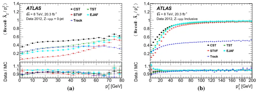
6.2 TheE_Tmissresponse . . . . 6.2.1 MeasuringE_Tmiss recoil versusp_TZ . . . . . 6.2.2 Measuring E_Tmiss response in simulated

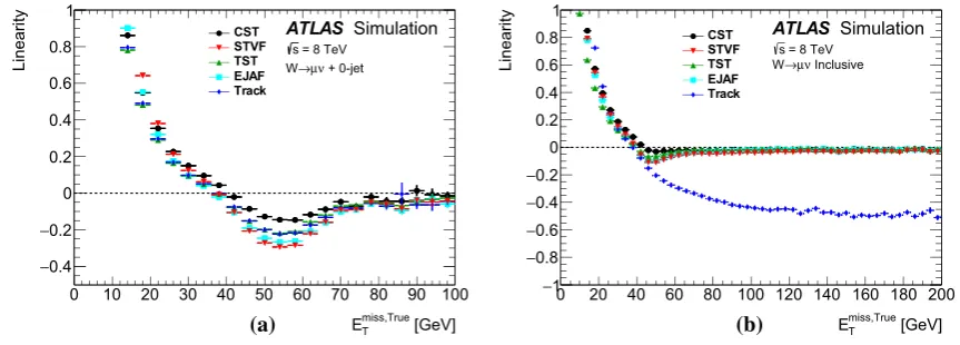
W →ν events . . . . 6.3 TheE_Tmissangular resolution . . . .

6.4 Transverse mass inW →ν events . . . .

6.5 Proxy forE_Tmisssignificance . . . . 6.6 Tails ofE_Tmiss distributions . . . . 6.7 Correlation of fakeE_Tmiss between algorithms . . 7 Jet-pT threshold and vertex association selection. . .

8 Systematic uncertainties of the soft term . . . . 8.1 Methodology for CST. . . .

8.1.1 Evaluation of balance between the soft term and the hard term . . . . 8.1.2 Cross-check method for the CST

system-atic uncertainties . . . . 8.2 Methodology for TST and TrackE_Tmiss . . . . 8.2.1 Propagation of systematic uncertainties . . 8.2.2 Closure of systematic uncertainties. . . . . 8.2.3 Systematic uncertainties from tracks inside

Appendix . . . . A. Calculation of EJAF . . . . References. . . .

1 Introduction

The Large Hadron Collider (LHC) provided proton–proton (pp) collisions at a centre-of-mass energy of 8 TeV during 2012. Momentum conservation transverse to the beam axis1 implies that the transverse momenta of all particles in the final state should sum to zero. Any imbalance may indicate the presence of undetectable particles such as neutrinos or new, stable particles escaping detection.

The missing transverse momentum (E_Tmiss) is recon-structed as the negative vector sum of the transverse momenta (pT) of all detected particles, and its magnitude is represented by the symbol Emiss_T . The measurement of Emiss_T strongly depends on the energy scale and resolution of the recon-structed “physics objects”. The physics objects considered in the E_Tmiss calculation are electrons, photons, muons,τ -leptons, and jets. Momentum contributions not attributed to any of the physics objects mentioned above are reconstructed as theE_Tmiss“soft term”. Several algorithms for reconstruct-ing theE_Tmisssoft term utilizing a combination of calorimeter signals and tracks in the inner detector are considered.

The E_Tmiss reconstruction algorithms and calibrations developed by ATLAS for 7 TeV data from 2010 are sum-marized in Ref. [1]. The 2011 and 2012 datasets are more affected by contributions from additional pp collisions, referred to as “pileup”, concurrent with the hard-scatter pro-cess. Various techniques have been developed to suppress such contributions. This paper describes the pileup depen-dence, calibration, and resolution of theE_Tmissreconstructed with different algorithms and pileup-mitigation techniques.

The performance of Emiss_T reconstruction algorithms, or “E_Tmiss performance”, refers to the use of derived quanti-ties like the mean, width, or tail of theEmiss_T distribution to study pileup dependence and calibration. The E_Tmiss recon-structed with different algorithms is studied in both data and Monte Carlo (MC) simulation, and the level of agreement between the two is compared using datasets in which events with a leptonically decayingWorZboson dominate. TheW boson sample provides events with intrinsicEmiss_T from non-interacting particles (e.g. neutrinos). Contributions to the E_Tmissdue to mismeasurement are referred to as fakeEmiss_T .

1_{ATLAS uses a right-handed coordinate system with its origin at the}

nominal interaction point (IP) in the centre of the detector and thez-axis along the beam pipe. Thex-axis points from the IP to the centre of the LHC ring, and they-axis points upward. Cylindrical coordinates(r, φ) are used in the transverse plane,φbeing the azimuthal angle around the beam pipe. The pseudorapidity is defined in terms of the polar angleθ asη= −ln tan(θ/2).

Sources of fake E_Tmiss may include pT mismeasurement, miscalibration, and particles going through un-instrumented regions of the detector. In MC simulations, the E_Tmissfrom each algorithm is compared to the true E_Tmiss (E_Tmiss,True), which is defined as the magnitude of the vector sum of pTof stable2weakly interacting particles from the hard-scatter col-lision. Then the selection efficiency after a E_Tmiss-threshold requirement is studied in simulated events with high-pT neu-trinos (such as top-quark pair production and vector-boson fusionH →ττ) or possible new weakly interacting particles that escape detection (such as the lightest supersymmetric particles).

This paper is organized as follows. Section2gives a brief introduction to the ATLAS detector. Section3describes the data and MC simulation used as well as the event selections applied. Section4 outlines how the E_Tmiss is reconstructed and calibrated while Sect.5presents the level of agreement between data and MC simulation inW andZboson produc-tion events. Performance studies of theE_Tmissalgorithms on data and MC simulation are shown for samples with different event topologies in Sect.6. The choice of jet selection crite-ria used in the E_Tmissreconstruction is discussed in Sect.7. Finally, the systematic uncertainty in the absolute scale and resolution of the Emiss

T is discussed in Sect. 8. To provide a reference, Table1 summarizes the different E_Tmiss terms discussed in this paper.

2 ATLAS detector

The ATLAS detector [2] is a multi-purpose particle physics apparatus with a forward-backward symmetric cylindrical geometry and nearly 4π coverage in solid angle. For track-ing, the inner detector (ID) covers the pseudorapidity range of|η|<2.5, and consists of a silicon-based pixel detector, a semiconductor tracker (SCT) based on microstrip technol-ogy, and, for|η|<2.0, a transition radiation tracker (TRT). The ID is surrounded by a thin superconducting solenoid pro-viding a 2 T magnetic field, which allows the measurement of the momenta of charged particles. A high-granularity elec-tromagnetic sampling calorimeter based on lead and liquid argon (LAr) technology covers the region of |η| < 3.2. A hadronic calorimeter based on steel absorbers and plastic-scintillator tiles provides coverage for hadrons, jets, andτ -leptons in the range of|η| <1.7. LAr technology using a copper absorber is also used for the hadronic calorimeters in the end-cap region of 1.5<|η|<3.2 and for electromag-netic and hadronic measurements with copper and tungsten absorbing materials in the forward region of 3.1<|η|<4.9. The muon spectrometer (MS) surrounds the calorimeters. It

2 _{ATLAS defines stable particles as those having a mean lifetime>}

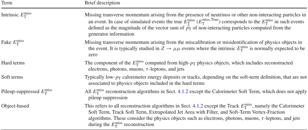
Table 1 Summary of definitions forEmiss

T terms used in this paper

Term Brief description

IntrinsicE_Tmiss Missing transverse momentum arising from the presence of neutrinos or other non-interacting particles in an event. In case of simulated events the trueEmiss

T (E

miss,True

T ) corresponds to theEmissT in such events

defined as the magnitude of the vector sum ofpTof non-interacting particles computed from the

generator information FakeEmiss

T Missing transverse momentum arising from the miscalibration or misidentification of physics objects in

the event. It is typically studied inZ→μμevents where the intrinsicEmiss

T is normally expected to be

zero

Hard terms The component of theEmiss

T computed from high-pTphysics objects, which includes reconstructed

electrons, photons, muons,τ-leptons, and jets

Soft terms Typically low-pTcalorimeter energy deposits or tracks, depending on the soft-term definition, that are not

associated to physics objects included in the hard terms

Pileup-suppressedE_Tmiss AllE_Tmissreconstruction algorithms in Sect.4.1.2except the Calorimeter Soft Term, which does not apply pileup suppression

Object-based This refers to all reconstruction algorithms in Sect.4.1.2except the TrackEmiss_T , namely the Calorimeter Soft Term, Track Soft Term, Extrapolated Jet Area with Filter, and Soft-Term Vertex-Fraction algorithms. These consider the physics objects such as electrons, photons, muons,τ-leptons, and jets during theEmiss

T reconstruction

consists of three air-core superconducting toroid magnet sys-tems, precision tracking chambers to provide accurate muon tracking out to|η| =2.7, and additional detectors for trig-gering in the region of|η|<2.4. A precision measurement of the track coordinates is provided by layers of drift tubes at three radial positions within|η|<2.0. For 2.0<|η|<2.7, cathode-strip chambers with high granularity are instead used in the innermost plane. The muon trigger system consists of resistive-plate chambers in the barrel (|η|<1.05) and thin-gap chambers in the end-cap regions (1.05<|η|<2.4).

3 Data samples and event selection

ATLAS recordedppcollisions at a centre-of-mass energy of 8 TeV with a bunch crossing interval (bunch spacing) of 50 ns in 2012. The resulting integrated luminosity is 20.3 fb−1[3]. Multiple inelastic pp interactions occurred in each bunch crossing, and the mean number of inelastic collisions per bunch crossing (μ) over the full dataset is 21 [4], excep-tionally reaching as high as about 70.

Data are analysed only if they satisfy the standard ATLAS data-quality assessment criteria [5]. Jet-cleaning cuts [5] are applied to minimize the impact of instrumental noise and out-of-time energy deposits in the calorimeter from cosmic rays or beam-induced backgrounds. This ensures that the residual sources ofE_Tmissmismeasurement due to those instrumental effects are suppressed.

3.1 Track and vertex selection

The ATLAS detector measures the momenta of charged parti-cles using the ID [6]. Hits from charged particles are recorded

and are used to reconstruct tracks; these are used to recon-struct vertices [7,8].

Each vertex must have at least two tracks with pT > 0.4 GeV; for the primary hard-scatter vertex (PV), the requirement on the number of tracks is raised to three. The PV in each event is selected as the vertex with the largest value of (pT)2, where the scalar sum is taken over all the tracks matched to the vertex. The following track selection criteria3 _{[7] are used throughout this paper, including the} vertex reconstruction:

• pT>0.5 GeV (0.4 GeV for vertex reconstruction and the calorimeter soft term),

• |η|<2.5,

• Number of hits in the pixel detector≥1,

• Number of hits in the SCT≥6.

These tracks are then matched to the PV by applying the following selections:

• |d0|<1.5 mm, • |z0sin(θ)|<1.5 mm.

The transverse (longitudinal) impact parameter d0 (z0)is the transverse (longitudinal) distance of the track from the PV and is computed at the point of closest approach to the PV in the plane transverse to the beam axis. The require-ments on the number of hits ensures that the track has an

3 _{The track reconstruction for electrons and for muons does not strictly}

accurate pT measurement. The|η|requirement keeps only the tracks within the ID acceptance, and the requirement of pT>0.4 GeV ensures that the track reaches the outer layers of the ID. Tracks with lowpThave large curvature and are more susceptible to multiple scattering.

The average spread along the beamline direction forpp collisions in ATLAS during 2012 data taking is around 50 mm, and the typical track z0 resolution for those with |η| < 0.2 and 0.5 < pT < 0.6 GeV is 0.34 mm. The typical trackd0resolution is around 0.19 mm for the sameη andpTranges, and both thez0andd0resolutions improve with higher trackpT.

Pileup effects come from two sources: in-time and out-of-time. In-time pileup is the result of multipleppinteractions in the same LHC bunch crossing. It is possible to distinguish the in-time pileup interactions by using their vertex posi-tions, which are spread along the beam axis. Atμ =21, the efficiency to reconstruct and select the correct vertex for Z→μμsimulated events is around 93.5% and rises to more than 98% when requiring two generated muons withpT>10 GeV inside the ID acceptance [10]. When vertices are sepa-rated along the beam axis by a distance smaller than the posi-tion resoluposi-tion, they can be reconstructed as a single vertex. Each track in the reconstructed vertex is assigned a weight based upon its compatibility with the fitted vertex, which depends on theχ2of the fit. The fraction of Z→μμ recon-structed vertices with more than 50% of the sum of track weights coming from pileup interactions is around 3% at

μ =21 [7,10]. Out-of-time pileup comes from pp colli-sions in earlier and later bunch crossings, which leave signals in the calorimeters that can take up to 450 ns for the charge collection time. This is longer than the 50 ns between subse-quent collisions and occurs because the integration time of the calorimeters is significantly larger than the time between the bunch crossings. By contrast the charge collection time of the silicon tracker is less than 25 ns.

3.2 Event selection for Z→

The “standard candle” for evaluation of the E_Tmiss perfor-mance is Z → events ( =eor μ). They are produced without neutrinos, apart from a very small number originat-ing from heavy-flavour decays in jets produced in association with theZ boson. The intrinsicE_Tmissis therefore expected to be close to zero, and the Emiss_T distributions are used to evaluate the modelling of the effects that give rise to fake E_Tmiss.

Candidate Z → events are required to pass an elec-tron or muon trigger [11,12]. The lowestpTthreshold for the unprescaled single-electron (single-muon) trigger ispT>25 (24) GeV, and both triggers apply a track-based isolation as well as quality selection criteria for the particle

identifica-tion. Triggers with higher pT thresholds, without the isola-tion requirements, are used to improve acceptance at high pT. These triggers require pT>60 (36) GeV for electrons (muons). Events are accepted if they pass any of the above trigger criteria. Each event must contain at least one primary vertex with azdisplacement from the nominalppinteraction point of less than 200 mm and with at least three associated tracks.

The offline selection of Z → μμ events requires the presence of exactly two identified muons [13]. An identi-fied muon is reconstructed in the MS and is matched to a track in the ID. The combined ID+MS track must have pT > 25 GeV and |η| < 2.5. The z displacement of the muon track from the primary vertex is required to be less than 10 mm. An isolation criterion is applied to the muon track, where the scalar sum of the pT of additional tracks within a cone of sizeR=(η)2_+(φ)2_{=0.2 around} the muon is required to be less than 10% of the muon pT. In addition, the two leptons are required to have oppo-site charge, and the reconstructed dilepton invariant mass, m, is required to be consistent with the Z boson mass: 66<m<116 GeV.

TheEmiss_T modelling and performance results obtained in Z→ μμandZ →eeevents are very similar. For the sake of brevity, only the Z → μμdistributions are shown in all sections except for Sect.6.6.

3.3 Event selection forW →ν

Leptonically decaying W bosons (W → ν) provide an important event topology with intrinsic E_Tmiss; the E_Tmiss distribution for such events is presented in Sect. 5.2. Sim-ilar to Z → events, a sample dominated by leptoni-cally decayingW bosons is used to study theEmiss_T scale in Sect.6.2.2, the resolution of theE_Tmissdirection in Sect.6.3, and the impact on a reconstructed kinematic observable in Sect.6.4.

The E_Tmissdistributions forW boson events in Sect.5.2 use the electron final state. These electrons are selected with

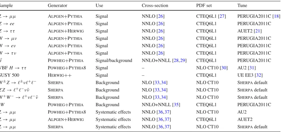
Table 2 Generators, cross-section normalizations, PDF sets, and MC tunes used in this analysis

Sample Generator Use Cross-section PDF set Tune

Z→μμ Alpgen+Pythia Signal NNLO [26] CTEQ6L1 [27] PERUGIA2011C [18]

Z→ee Alpgen+Pythia Signal NNLO [26] CTEQ6L1 PERUGIA2011C

Z→ττ Alpgen+Herwig Signal NNLO [26] CTEQ6L1 AUET2 [21]

W→μν Alpgen+Pythia Signal NNLO [26] CTEQ6L1 PERUGIA2011C

W→eν Alpgen+Pythia Signal NNLO [26] CTEQ6L1 PERUGIA2011C

W→τν Alpgen+Pythia Signal NNLO [26] CTEQ6L1 PERUGIA2011C

tt¯ Powheg+Pythia Signal/background NNLO+NNLL [28,29] CTEQ6L1 PERUGIA2011C

VBFH→ττ Powheg+Pythia8 Signal – NLO CT10 [30] AU2 [31]

SUSY 500 Herwig++ Signal – CTEQ6L1 UE EE3 [32]

W±Z→±ν+− Sherpa Background NLO [33,34] NLO CT10 Sherpadefault

Z Z →+−νν¯ Sherpa Background NLO [33,34] NLO CT10 Sherpadefault

W+W−→+ν−ν¯ Sherpa Background NLO [33,34] NLO CT10 Sherpadefault

t W Powheg+Pythia Background NNLO+NNLL [35] CTEQ6L1 PERUGIA2011C

Z→μμ Powheg+Pythia8 Systematic effects NNLO [36,37] NLO CT10 AU2

Z→μμ Alpgen+Herwig Systematic effects NNLO [36,37] CTEQ6L1 AUET2

Z→μμ Sherpa Systematic effects NNLO [36,37] NLO CT10 Sherpadefault

electron tracks are then matched to the PV by applying the following selections:

• |d0|<5.0 mm, • |z0sin(θ)|<0.5 mm.

TheW boson selection is based on the single-lepton trig-gers and the same lepton selection criteria as those used in the Z→ selection. Events are rejected if they contain more than one reconstructed lepton. Selections on theE_Tmissand transverse mass (mT) are applied to reduce the multi-jet back-ground with one jet misidentified as an isolated lepton. The transverse mass is calculated from the lepton and theE_Tmiss,

mT=

2p_TEmiss_T (1−cosφ), (1)

wherep_Tis the transverse momentum of the lepton andφis the azimuthal angle between the lepton andEmiss_T directions. Both themTandETmissare required to be greater than 50 GeV. These selections can bias the event topology and its phase space, so they are only used when comparing simulation to data in Sect.5.2, as they substantially improve the purity of W bosons in data events.

TheE_Tmissmodelling and performance results obtained in W →eνandW →μνevents are very similar. For the sake of brevity, only one of the two is considered in following two sections:E_Tmissdistributions inW →eνevents are presented in Sect.5.2and the performance studies show W → μν events in Sect.6. When studying the Emiss_T tails, both final states are considered in Sect.6.6, because theη-coverage

and reconstruction performance between muons and elec-trons differ.

3.4 Monte Carlo simulation samples

Table2summarizes the MC simulation samples used in this paper. The Z→andW →νsamples are generated with

Alpgen_{[16] interfaced with}Pythia_{[17] (denoted by} Alp-gen₊Pythia_{) to model the parton shower and hadronization,}

and underlying event using the PERUGIA2011C set [18] of tunable parameters. One exception is the Z → ττ sample with leptonically decayingτ-leptons, which is generated with

Alpgen _{interfaced with} Herwig_{[19] with the underlying}

event modelled usingJimmy[20] and the AUET2 tunes [21].

Alpgen_{is a multi-leg generator that provides tree-level}

cal-culations for diagrams with up to five additional partons. The matrix-element MC calculations are matched to a model of the parton shower, underlying event and hadronization. The main processes that are backgrounds to Z → and W → ν are events with one or more top quarks (tt¯and single-top-quark processes) and diboson production (W W, W Z, Z Z). The tt¯ and t W processes are generated with

Powheg_{[22] interfaced with}Pythia_{[17] for hadronization}

and parton showering, and PERUGIA2011C for the underly-ing event modellunderly-ing. All the diboson processes are generated withSherpa[23].Powhegis a leading-order generator with corrections at next-to-leading order inαS, whereasSherpa is a multi-leg generator at tree level.

with at least one leptonically decayingW boson are consid-ered in Sect.6.6. The single top quark (t W) production is considered with at least one leptonically decayingWboson. Both thett¯andt Wprocesses contribute to theWandZboson distributions shown in Sect.5as well as Z boson distribu-tions in Sects.4,6, and8that compare data and simulation. A supersymmetric (SUSY) model comprising pair-produced 500 GeV gluinos each decaying to att¯pair and a neutralino is simulated with Herwig++[24]. Finally, to study events with forward jets, the vector-boson fusion (VBF) produc-tion ofH→ττ, generated withPowheg+Pythia8[25], is considered. Bothτ-leptons are forced to decay leptonically in this sample.

To estimate the systematic uncertainties in the data/MC ratio arising from the modelling of the soft hadronic recoil, E_Tmiss distributions simulated with different MC generators, parton shower and underlying event models are compared. The estimation of systematic uncertainties is performed using a comparison of data and MC sim-ulation, as shown in Sect. 8.2. The following combina-tions of generators and parton shower models are consid-ered: Sherpa, Alpgen+Herwig, Alpgen+Pythia, and

Powheg_+Pythia8_{. The corresponding underlying event}

tunes are mentioned in Table2. Parton distribution functions are taken fromCT10[30] forPowhegandSherpasamples andCTEQ6L1[38] forAlpgensamples.

Generated events are propagated through a Geant4 sim-ulation [39,40] of the ATLAS detector. Pileup collisions are generated with Pythia8for all samples, and are overlaid on top of simulated hard-scatter events before event reconstruc-tion. Each simulation sample is weighted by its correspond-ing cross-section and normalized to the integrated luminosity of the data.

4 Reconstruction and calibration of theE_Tmiss

Several algorithms have been developed to reconstruct the E_Tmissin ATLAS. They differ in the information used to recon-struct thepTof the particles, using either energy deposits in the calorimeters, tracks reconstructed in the ID, or both. This section describes these various reconstruction algorithms, and the remaining sections discuss the agreement between data and MC simulation as well as performance studies.

4.1 Reconstruction of theE_Tmiss

TheE_Tmissreconstruction uses calibrated physics objects to estimate the amount of missing transverse momentum in the detector. TheE_Tmissis calculated using the components along thexandyaxes:

E_xmiss_(y) =Emiss_x(y),e+E_xmiss_(y),γ +E_xmiss_(y),τ

+Emiss_x(y),jets+E_xmiss_(y),μ+Emiss_x(y),soft, (2)

where each term is calculated as the negative vectorial sum of transverse momenta of energy deposits and/or tracks. To avoid double counting, energy deposits in the calorimeters and tracks are matched to reconstructed physics objects in the following order: electrons (e), photons (γ), the visible parts of hadronically decayingτ-leptons (τhad-vis; labelled asτ), jets and muons (μ). Each type of physics object is represented by a separate term in Eq. (2). The signals not associated with physics objects form the “soft term”, whereas those associated with the physics objects are collectively referred to as the “hard term”.

The magnitude and azimuthal angle4(φmiss) ofE_Tmissare calculated as:

E_Tmiss=

(Emiss

x )2+(Emissy )2, φmiss_=arctan(Emiss

y /Emissx ).

(3)

The total transverse energy in the detector, labelled asET, quantifies the total event activity and is an important observ-able for understanding the resolution of theE_Tmiss, especially with increasing pileup contributions. It is defined as:

ET=

p_Te +p_Tγ+p_Tτ+p_Tjets

+pμ_T+psoft_T , (4)

which is the scalar sum of the transverse momenta of recon-structed physics objects and soft-term signals that contribute to theE_Tmissreconstruction. The physics objects included in

psoft_T depend on theEmiss_T definition, so both calorimeter objects and track-based objects may be included in the sum, despite differences in pTresolution.

4.1.1 Reconstruction and calibration of the E_Tmisshard terms

The hard term of the Emiss_T , which is computed from the reconstructed electrons, photons, muons,τ-leptons, and jets, is described in more detail in this section.

Electrons are reconstructed from clusters in the electro-magnetic (EM) calorimeter which are associated with an ID track [14]. Electron identification is restricted to the range of

|η|<2.47, excluding the transition region between the barrel and end-cap EM calorimeters, 1.37<|η|<1.52. They are calibrated at the EM scale5with the default electron

calibra-4 _{The arctan function returns values from[−π,+π]and uses the sign}

of both coordinates to determine the quadrant.

5 _{The EM scale is the basic signal scale for the ATLAS}

tion, and those satisfying the “medium” selection criteria [14] withpT>10 GeV are included in theE_Tmissreconstruction. The photon reconstruction is also seeded from clusters of energy deposited in the EM calorimeter and is designed to separate electrons from photons. Photons are calibrated at the EM scale and are required to satisfy the “tight” photon selection criteria with pT>10 GeV [14].

Muon candidates are identified by matching an ID track with an MS track or segment [13]. MS tracks are used for 2.5<|η|<2.7 to extend theηcoverage. Muons are required to satisfy pT >5 GeV to be included in the E_Tmiss recon-struction. The contribution of muon energy deposited in the calorimeter is taken into account using either parameterized estimates or direct measurements, to avoid double counting a small fraction of their momenta.

Jets are reconstructed from three-dimensional topolog-ical clusters (topoclusters) [41] of energy deposits in the calorimeter using the anti-kt algorithm [42] with a distance parameterR=0.4. The topological clustering algorithm sup-presses noise by forming contiguous clusters of calorime-ter cells with significant energy deposits. The local clus-ter weighting (LCW) [43,44] calibration is used to account for different calorimeter responses to electrons, photons and hadrons. Each cluster is classified as coming from an EM or hadronic shower, using information from its shape and energy density, and calibrated accordingly. The jets are reconstructed from calibrated topoclusters and then corrected for in-time and out-of-time pileup as well as the position of the PV [4]. Finally, the jet energy scale (JES) corrects for jet-level effects by restoring, on average, the energy of reconstructed jets to that of the MC generator-level jets. The complete procedure is referred to as the LCW+JES scheme [43,44]. Without chang-ing the average calibration, additional corrections are made based upon the internal properties of the jet (global sequen-tial calibration) to reduce the flavour dependence and energy leakage effects [44]. Only jets with calibratedpTgreater than 20 GeV are used to calculate the jet termE_xmiss_(y),jetsin Eq. (2), and the optimization of the 20 GeV threshold is discussed in Sect.7.

To suppress contributions from jets originating from pileup interactions, a requirement on the jet vertex-fraction (JVF) [4] may be applied to selected jet candidates. Tracks matched to jets are extrapolated back to the beamline to ascer-tain whether they originate from the hard scatter or from a pileup collision. The JVF is then computed as the ratio shown below:

JVF=

track,PV,jet

pT/

track,jet

pT. (5)

This is the ratio of the scalar sum of transverse momentum of all tracks matched to the jet and the primary vertex to the pT sum of all tracks matched to the jet, where the sum is performed over all tracks withpT>0.5 GeV and|η|<2.5

and the matching is performed using the “ghost-association” procedure [45,46].

The JVF distribution is peaked toward 1 for hard-scatter jets and toward 0 for pileup jets. No JVF selection require-ment is applied to jets that have no associated tracks. Require-ments on the JVF are made in the STVF, EJAF, and TST E_Tmissalgorithms as described in Table3and Sect.4.1.3.

Hadronically decayingτ-leptons are seeded by calorime-ter jets with|η|<2.5 and pT >10 GeV. As described for jets, the LCW calibration is applied, corrections are made to subtract the energy due to pileup interactions, and the energy of the hadronically decaying τ candidates is calibrated at theτ-lepton energy scale (TES) [47]. The TES is indepen-dent of the JES and is determined using an MC-based proce-dure. Hadronically decayingτ-leptons passing the “medium” requirements [47] and havingpT>20 GeV after TES cor-rections are considered for theEmiss_T reconstruction.

4.1.2 Reconstruction and calibration of the E_Tmisssoft term

The soft term is a necessary but challenging ingredient of the Emiss_T reconstruction. It comprises all the detector sig-nals not matched to the physics objects defined above and can contain contributions from the hard scatter as well as the underlying event and pileup interactions. Several algorithms designed to reconstruct and calibrate the soft term have been developed, as well as methods to suppress the pileup contri-butions. A summary of theEmiss_T and soft-term reconstruction algorithms is given in Table3.

Four soft-term reconstruction algorithms are considered in this paper. Below the first two are defined, and then some motivation is given for the remaining two prior to their defi-nition.

• Calorimeter Soft Term (CST)

Table 3 Summary ofEmiss

T and soft-term reconstruction algorithms used in this paper

Term Brief description Section list

CSTE_Tmiss The Calorimeter Soft Term (CST)E_Tmisstakes its soft term from energy deposits in the calorimeter which are not matched to high-pTphysics objects. Although noise

suppression is applied to reduce fake signals, no additional pileup suppression techniques are used

Section4.1.2(definition) Section5.1(Z→μμmodelling) Section5.2(W→eνmodelling) Section6(perf. studies) TSTE_Tmiss The Track Soft Term (TST)Emiss_T algorithm uses a soft term that is calculated using

tracks within the inner detector that are not associated with high-p_Tphysics objects. The JVF selection requirement is applied to jets

Section4.1.2(definition) Section5.1(Z→μμmodelling) Section5.2(W→eνmodelling) Section6(perf. studies) EJAFEmiss

T The Extrapolated Jet Area with FilterEmissT algorithm applies pileup subtraction to

the CST based on the idea of jet-area corrections. The JVF selection requirement is applied to jets

Section4.1.2(definition) Section5.1(Z→μμmodelling) Section6(perf. studies) STVFEmiss

T The Soft-Term Vertex-Fraction (STVF)EmissT algorithm suppresses pileup effects in

the CST by scaling the soft term by a multiplicative factor calculated based on the fraction of scalar-summed trackpTnot associated with high-pTphysics objects

that can be matched to the primary vertex. The JVF selection requirement is applied to jets

Section4.1.2(definition) Section5.1(Z→μμmodelling) Section6(perf. studies)

TrackE_Tmiss The TrackE_Tmissis reconstructed entirely from tracks to avoid pileup contamination that affects the other algorithms

Section4.2(definition)

Section5.1(Z→μμmodelling) Section6(perf. studies)

with pT > 0.4 GeV that are not matched to a

high-pT physics objects are used instead of the calorimeter

pTmeasurement, if theirpTresolution is better than the expected calorimeterpTresolution. The calorimeter res-olution is estimated as 0.4· √pTGeV, in which thepTis the transverse momentum of the reconstructed track. Geometrical matching between tracks and topoclusters (or high-pTphysics objects) is performed using theR significance defined asR/σR, whereσRis theR resolution, parameterized as a function of the track pT. A track is considered to be associated to a topocluster in the soft term when its minimumR/σRis less than 4. To veto tracks matched to high-pTphysics objects, tracks are required to haveR/σR>8. TheE_Tmisscalculated using the CST algorithm is documented in previous pub-lications such as Ref. [1] and is the standard algorithm in most ATLAS 8 TeV analyses.

• Track Soft Term (TST)

The TST is reconstructed purely from tracks that pass the selections outlined in Sect.3.1and are not associated with the high-pT physics objects defined in Sect.4.1.1. The detector coverage of the TST is the ID tracking vol-ume (|η|<2.5), and no calorimeter topoclusters inside or beyond this region are included. This algorithm allows excellent vertex matching for the soft term, which almost completely removes the in-time pileup dependence, but misses contributions from soft neutral particles. The track-based reconstruction also entirely removes the out-of-time pileup contributions that affect the CST.

To avoid double counting the pTof particles, the tracks matched to the high-pT physics objects need to be removed from the soft term. All of the following classes of tracks are excluded from the soft term:

– tracks within a cone of sizeR=0.05 around elec-trons and photons

– tracks within a cone of sizeR=0.2 aroundτhad-vis

– ID tracks associated with identified muons

– tracks matched to jets using the ghost-association technique described in Sect.4.1.1

– isolated tracks with pT ≥ 120 GeV (≥200 GeV for |η|<1.5) having transverse momentum uncertainties larger than 40% or having no associated calorime-ter energy deposit with pT larger than 65% of the trackpT. ThepTthresholds are chosen to ensure that muons not in the coverage of the MS are still included in the soft term. This is a cleaning cut to remove mis-measured tracks.

The TST algorithm is very stable with respect to pileup but does not include neutral particles. Two other pileup-suppressing algorithms were developed, which consider con-tributions from neutral particles. One uses anη-dependent event-by-event estimator for the transverse momentum den-sity from pileup, using calorimeter information, while the other applies an event-by-event global correction based on the amount of charged-particlepTfrom the hard-scatter ver-tex, relative to all otherppcollisions. The definitions of these two soft-term algorithms are described in the following:

• Extrapolated Jet Area with Filter (EJAF)

The jet-area method for the pileup subtraction uses a soft term based on the idea of jet-area corrections [45]. This technique uses direct event-by-event measurements of the energy flow throughout the entire ATLAS detector to estimate thepTdensity of pileup energy deposits and was

developed from the strategy applied to jets as described in Ref. [4].

The topoclusters belonging to the soft term are used for jet finding with the kt algorithm [48,49] with dis-tance parameterR=0.6 and jetpT>0. The catchment areas [45,46] for these reconstructed jets are labelled Ajet; this provides a measure of the jet’s susceptibility to contamination from pileup. Jets withpT<20 GeV are referred to as soft-term jets, and the pT-density of each soft-term jetiis then measured by computing:

ρjet,i = pjet_T,i

Ajet,i.

(6)

In a given event, the medianpT-densityρevtmedfor all soft-termktjets in the event (Njets) found within a given range −ηmax< ηjet< ηmaxcan be calculated as

ρmed

evt =median{ρjet,i} fori=1. . .Njetsin|ηjet|< ηmax.

(7)

This medianpT-densityρevtmedgives a good estimate of the in-time pileup activity in each detector region. If deter-mined with ηmax =2, it is found to also be an appro-priate indicator of out-of-time pileup contributions [45]. A lower value forρevtmedis computed by using jets with |ηjet|larger than 2, which is mostly due to the particular

geometry of the ATLAS calorimeters and their cluster reconstruction algorithms.6

In order to extrapolate ρ_evtmed into the forward regions of the detector, the average topocluster pT in slices of

η,NPV, andμ is converted to an average pTdensity ρ(η,NPV, μ) for the soft term. As described for the

ρmed

evt ,ρ(η,NPV, μ)is found to be uniform in the cen-tral region of the detector with|η|< ηplateau=1.8. The transverse momentum density profile is then computed as

Pρ(η,NPV,μ)= ρ(η,

NPV, μ) ρcentral(NPV, μ)

(8)

whereρcentral(NPV, μ) is the averageρ(η,NPV, μ) for|η|< ηplateau. ThePρ(η,NPV,μ)is therefore 1, by definition, for|η|< ηplateauand decreases for larger|η|. A functional form ofPρ(η,NPV,μ)is used to param-eterize its dependence onη,NPV, andμand is defined as

P_fctρ(η,NPV,μ)=

1 (|η| < ηplateau)

(1−Gbase(ηplateau))·Gcore(|η| −ηplateau)+Gbase(η)

|η| ≥ ηplateau

(9)

where the central region|η|< ηplateau=1.8 is plateaued at 1, and then a pair of Gaussian functionsGcore(|η| −

ηplateau)andGbase(η)are added for the fit in the forward regions of the calorimeter. The value ofGcore(0) = 1 so that Eq. (9) is continuous atη = ηplateau. Two exam-ple fits are shown in Fig. 1 for NPV = 3 and 8 with μ =7.5–9.5 interactions per bunch crossing. For both distributions the value is defined to be unity in the cen-tral region (|η|< ηplateau), and the sum of two Gaussian functions provides a good description of the change in the amount of in-time pileup beyondηplateau. The base-line Gaussian functionGbase(η)has a larger width and is used to describe the larger amount of in-time pileup in the forward region as seen in Fig.1. Fitting with Eq. (9) provides a parameterized function for in-time and out-of-time pileup which is valid for the whole 2012 dataset. The soft term for the EJAFE_Tmissalgorithm is calcu-lated as

Emiss_x(y),soft= − Nfilter-jet

i=0

pjet_x(y,corr_),i , (10)

which sums the transverse momenta, labelledpjet_x(y,corr_),i , of the corrected soft-term jets matched to the primary ver-tex. The number of these filtered jets, which are selected

6 _{The forward ATLAS calorimeters are less granular than those in the}

η

4

− −2 0 2 4

) 〉μ〈 , PV ,N η ( ρ P 2 − 10 1 − 10 1 ATLAS Data 2012

s=8TeV Minimum Bias,

< 9.5 〉 μ 〈 = 3, 7.5 <

PV N ) 〉 μ 〈 , PV ,N η ( fct ρ Fit of P

) 〉 μ 〈 , PV (N base

Fit of G

(a) η

4

− −2 0 2 4

2 − 10 1 − 10 1 ATLAS Data 2012

s=8TeV Minimum Bias, (b) ) 〉μ〈 , PV ,N η ( ρ P < 9.5 〉 μ 〈 = 8, 7.5 <

PV N ) 〉 μ 〈 , PV ,N η ( fct ρ Fit of P

) 〉 μ 〈 , PV (N base

Fit of G

Fig. 1 The average transverse momentum density shape Pρ(η,NPV,μ)for jets in data is compared to the model in Eq. (9)

withμ = 7.5–9.5 and with a three reconstructed vertices and b

eight reconstructed vertices. The increase of jet activity in the forward

regions coming from more in-time pileup with NPV=8 inbcan be

seen by the flatter shape of the Gaussian fit of the forward activity Gbase(NPV,μ)(blue dashed line)

after the pileup correction based on their JVF andpT, is labelledNfilter-jet. More details of the jet selection and the application of the pileup correction to the jets are given in Appendix A.

• Soft-Term Vertex-Fraction (STVF)

The algorithm, called the soft-term vertex-fraction, uti-lizes an event-level parameter computed from the ID track information, which can be reliably matched to the hard-scatter collision, to suppress pileup effects in the CST. This correction is applied as a multiplicative fac-tor (αSTVF) to the CST, event by event, and the resulting STVF-corrected CST is simply referred to as STVF. The

αSTVFis calculated as

αSTVF=

tracks,PV

pT

tracks

pT, (11)

which is the scalar sum ofpTof tracks matched to the PV divided by the total scalar sum of track pTin the event, including pileup. The sums are taken over the tracks that do not match high-pTphysics objects belonging to the hard term. The meanαSTVF value is shown versus the number of reconstructed vertices (NPV) in Fig.2. Data and simulation (including Z, diboson,tt¯, andt W sam-ples) are shown with only statistical uncertainties and agree within 4–7% across the full range of NPV in the 8 TeV dataset. The differences mostly arise from the mod-elling of the amount of the underlying event and p_TZ. The 0-jet and inclusive samples have similar values of

αSTVF, with that for the inclusive sample being around 2% larger.

0 5 10 15 20 25 30

〉 STVF α〈 1 − 10 1 Inclusive 0-jet ATLAS -1

= 8 TeV, 20.3 fb s

μμ → Data 2012, Z

) PV Number of Reconstructed Vertices (N

0 5 10 15 20 25 30

Data / MC

0.951

1.05

Fig. 2 The meanαSTVFweight is shown versus the number of

recon-structed vertices (NPV) for 0-jet and inclusive events in Z→μμdata.

Theinsetat thebottomof the figure shows the ratio of the data to the MC predictions with only the statistical uncertainties on the data and MC simulation. The bin boundary always includes the lower edge and not the upper edge

4.1.3 Jet pTthreshold and JVF selection

The TST, STVF, and EJAF E_Tmiss algorithms complement the pileup reduction in the soft term with additional require-ments on the jets entering theEmiss_T hard term, which are also aimed at reducing pileup dependence. These E_Tmiss recon-struction algorithms apply a requirement of JVF>0.25 to jets with pT<50 GeV and|η|<2.4 in order to suppress those originating from pileup interactions. The maximum

parti-cles from jets below the pT threshold are considered in the soft terms for the STVF, TST, and EJAF (see Sect.4.1.2for details).

The same JVF requirements are not applied to the CST E_Tmissbecause its soft term includes the soft recoil from all interactions, so removing jets not associated with the hard-scatter interaction could create an imbalance. The procedure for choosing the jet pT and JVF criteria is summarized in Sect.7.

Throughout most of this paper the number of jets is com-puted without a JVF requirement so that theE_Tmissalgorithms are compared on the same subset of events. However, the JVF>0.25 requirement is applied in jet counting when 1-jet and≥2-jet samples are studied using the TST E_Tmiss recon-struction, which includes Figs.8and22. The JVF removes pileup jets that obscure trends in samples with different jet multiplicities.

4.2 TrackE_Tmiss

Extending the philosophy of the TST definition to the full event, the E_Tmiss is reconstructed from tracks alone, reduc-ing the pileup contamination that afflicts the other object-based algorithms. While a purely track-object-basedEmiss_T , desig-nated Track E_Tmiss, has almost no pileup dependence, it is insensitive to neutral particles, which do not form tracks in the ID. This can degrade the E_Tmiss calibration, espe-cially in event topologies with numerous or highly ener-getic jets. Theη coverage of the Track Emiss_T is also lim-ited to the ID acceptance of |η| < 2.5, which is substan-tially smaller than the calorimeter coverage, which extends to

|η| =4.9.

TrackE_Tmissis calculated by taking the negative vectorial sum ofpTof tracks satisfying the same quality criteria as the TST tracks. Similar to the TST, tracks with poor momentum resolution or without corresponding calorimeter deposits are removed. Because of Bremsstrahlung within the ID, the elec-tronpTis determined more precisely by the calorimeter than by the ID. Therefore, the TrackE_Tmissalgorithm uses the elec-tronpTmeasurement in the calorimeter and removes tracks overlapping its shower. Calorimeter deposits from photons are not added because they cannot be reliably associated to particularppinteractions. For muons, the ID trackpTis used and not the fits combining the ID and MSpT. For events with-out any reconstructed jets, the Track and TSTEmiss_T would have similar values, but differences could still originate from muon track measurements as well as reconstructed photons or calorimeter deposits fromτhad-vis, which are only included in the TST.

The soft term for the TrackE_Tmissis defined to be identical to the TST by excluding tracks associated with the high-pT physics objects used in Eq. (2).

5 Comparison of Emiss_T distributions in data and MC simulation

In this section, basic Emiss_T distributions before and after pileup suppression in Z→andW →νdata events are compared to the distributions from the MC signal plus rel-evant background samples. All distributions in this section include the dominant systematic uncertainties on the high-pT objects, the ETmiss,soft (described in Sect.8) and pileup modelling [7]. The systematics listed above are the largest systematic uncertainties in theE_Tmissfor ZandW samples.

5.1 Modelling of Z→events

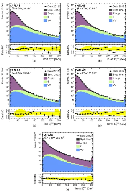
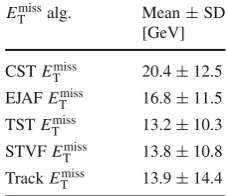
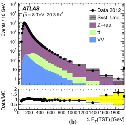
The CST, EJAF, TST, STVF, and Track E_Tmissdistributions for Z → μμdata and simulation are shown in Fig.3. The Z boson signal region, which is defined in Sect. 3.2, has better than 99% signal purity. The MC simulation agrees with data for allE_Tmissreconstruction algorithms within the assigned systematic uncertainties. The mean and the stan-dard deviation of the E_Tmiss distribution is shown for all of the E_Tmiss algorithms in Z → μμ inclusive simulation in Table 4. The CST E_Tmiss has the highest mean E_Tmiss and thus the broadest Emiss_T distribution. All of the E_Tmiss algo-rithms with pileup suppression have narrowerE_Tmiss distribu-tions as shown by their smaller meanEmiss_T values. However, those algorithms also have non-Gaussian tails in the E_xmiss andEmissy distributions, which contribute to the region with

E_Tmiss50 GeV. The TrackE_Tmisshas the largest tail because it does not include contributions from the neutral particles, and this results in it having the largest standard deviation.

The tails of the E_Tmiss distributions in Fig. 3 for Z → μμ data are observed to be compatible with the sum of expected signal and background contributions, namelytt¯and the summed diboson (V V) processes includingW W,W Z, andZ Z, which all have high-pTneutrinos in their final states. Instrumental effects can show up in the tails of theE_Tmiss, but such effects are small.

TheE_Tmissφdistribution is not shown in this paper but is very uniform, having less than 4 parts in a thousand differ-ence from positive and negativeφ. Thus theφ-asymmetry is greatly reduced from that observed in Ref. [1].

Events / 10 GeV 1 10 2 10 3 10 4 10 5 10 6 10 7 10 8 10 Data 2012 Syst. Unc. μ μ → Z t t VV ATLAS -1 = 8 TeV, 20.3 fb s

ATLAS

-1 = 8 TeV, 20.3 fb s

[GeV] miss T CST E 0 50 100 150 200 250 300

Data/MC 0.6

0.81 1.2 1.4

(a)

Events / 10 GeV

1 10 2 10 3 10 4 10 5 10 6 10 7 10 8 10 Data 2012 Syst. Unc. t t VV ATLAS -1 = 8 TeV, 20.3 fb s

ATLAS

-1 = 8 TeV, 20.3 fb s

[GeV] miss T EJAF E 0 50 100 150 200 250 300

Data/MC 0.6

0.81 1.2 1.4

(b)

Events / 10 GeV

1 10 2 10 3 10 4 10 5 10 6 10 7 10 8

10 _{Data 2012}

Syst. Unc. t t VV ATLAS -1 = 8 TeV, 20.3 fb s

ATLAS

-1 = 8 TeV, 20.3 fb s

[GeV] miss T TST E 0 50 100 150 200 250 300

Data/MC 0.60.8 1 1.2 1.4

(c)

Events / 10 GeV

1 10 2 10 3 10 4 10 5 10 6 10 7 10 8

10 _{Data 2012}

Syst. Unc. t t VV ATLAS -1 = 8 TeV, 20.3 fb s

ATLAS

-1 = 8 TeV, 20.3 fb s

[GeV] miss T STVF E 0 50 100 150 200 250 300

Data/MC 0.60.8 1 1.2 1.4

(d)

Events / 10 GeV

1 10 2 10 3 10 4 10 5 10 6 10 7 10 8

10 _{Data 2012}

Syst. Unc. t t VV ATLAS -1 = 8 TeV, 20.3 fb s

ATLAS

-1 = 8 TeV, 20.3 fb s

[GeV] miss T Track E 0 50 100 150 200 250 300

Data/MC 0.60.8 1 1.2 1.4 (e) μ μ → Z μ μ →

Z Z→μμ

μ μ → Z

Fig. 3 Distributions of theE_Tmisswith theaCST,bEJAF,cTST,d

STVF, andeTrackEmiss

T are shown in data and MC simulation events

satisfying the Z→μμselection. Thelower panel of the figuresshows

Table 4 The mean and standard deviation of the

Emiss

T distributions in

Z→μμinclusive simulation

Emiss

T alg. Mean±SD

[GeV] CSTEmiss

T 20.4±12.5

EJAFEmiss

T 16.8±11.5

TSTEmiss

T 13.2±10.3

STVFEmiss

T 13.8±10.8

TrackEmiss

T 13.9±14.4

causes the larger systematic uncertainty for the TST and STVFE_Tmiss. The TrackEmiss_T does not have the same increase in systematic uncertainties because it does not make use of reconstructed jets. Above 120 GeV, most events have a large

intrinsicEmiss_T , and the systematic uncertainties on theE_Tmiss, especially the soft term, are smaller.

Figure 4 shows the soft-term distributions. The pileup-suppressedEmiss_T algorithms generally have a smaller mean soft term as well as a sharper peak near zero compared to the CST. Among the Emiss_T algorithms, the soft term from the EJAF algorithm shows the smallest change relative to the CST. The TST has a sharp peak near zero similar to the STVF but with a longer tail, which mostly comes from individual tracks. These tracks are possibly mismeasured and further studies are planned. The simulation under-predicts the TST relative to the observed data between 60–85 GeV, and the dif-ferences exceed the assigned systematic uncertainties. This

[GeV]

miss T

CST E

0 50 100 150 200 250 300

Data/MC 0.60.8 1 1.2

1.4 h_tot_MET_xType0

Events / 4 GeV

1 10 2 10 3 10 4 10 5 10 6 10 7 10 8

10 Data 2012

Syst. Unc. μ μ → Z t t VV ATLAS -1 = 8 TeV, 20.3 fb s

ATLAS

-1 = 8 TeV, 20.3 fb s

[GeV]

miss,soft T

CST E

0 20 40 60 80 100 120 140 160

Data/MC 0 0.5 1 1.5 2

Events / 4 GeV

1 10 2 10 3 10 4 10 5 10 6 10 7 10 8

10 Data 2012

Syst. Unc. μ μ → Z t t VV ATLAS -1 = 8 TeV, 20.3 fb s

ATLAS

-1 = 8 TeV, 20.3 fb s

[GeV]

miss,soft T

EJAF E

0 20 40 60 80 100 120 140 160

Data/MC 0 0.5 1 1.5 2 [GeV] miss T TST E

0 50 100 150 200 250 300

Data/MC 0.60.8 1 1.2 1.4

h_tot_MET_TST_xType0

Events / 4 GeV

1 10 2 10 3 10 4 10 5 10 6 10 7 10 8

10 Data 2012

Syst. Unc. μ μ → Z t t VV ATLAS -1 = 8 TeV, 20.3 fb s

ATLAS

-1 = 8 TeV, 20.3 fb s

[GeV]

miss,soft T

TST E

0 20 40 60 80 100 120 140 160

Data/MC 0 0.51 1.5 2

Events / 4 GeV

1 10 2 10 3 10 4 10 5 10 6 10 7 10 8

10 Data 2012

Syst. Unc. μ μ → Z t t VV ATLAS -1 = 8 TeV, 20.3 fb s

ATLAS

-1 = 8 TeV, 20.3 fb s

[GeV]

miss,soft T

STVF E

0 20 40 60 80 100 120 140 160

Data/MC 0 0.51 1.5 2 (a) (b) (c) (d)

Fig. 4 Distributions of the soft term for theaCST,bEJAF,cTST, anddSTVF are shown in data and MC simulation events satisfying the Z→μμselection. Thelower panelof the figures show the ratio

miss T

CST E

0 50 100 150 200 250 300

0.6 0.8 1.2 1.4 h_tot_MET_xType0 [GeV] miss,soft T CST E

0 20 40 60 80 100 120 140 160 h_term_MET_xType3

Events / 10 GeV

1 10 2 10 3 10 4 10 5 10 6 10 7 10 8 10 Data 2012 Syst. Unc. μ μ → Z t t VV ATLAS -1 = 8 TeV, 20.3 fb s

(CST) [GeV]

T

E

Σ

0 200 400 600 800 1000 1200 1400 1600 1800

Data/MC 0 0.5 1 1.5 2 miss T TST E

0 50 100 150 200 250 300

0.6 0.8 1.2 1.4 h_tot_MET_TST_xType0 [GeV] miss,soft T TST E

0 20 40 60 80 100 120 140 160 h_term_MET_TST_xType3

Events / 10 GeV

1 10 2 10 3 10 4 10 5 10 6 10 7 10 8 10 Data 2012 Syst. Unc. μ μ → Z t t VV ATLAS -1 = 8 TeV, 20.3 fb s

(TST) [GeV]

T

E

Σ

0 200 400 600 800 1000 1200 1400 1600 1800

Data/MC 0 0.5 1 1.5 2 (a) (b)

Fig. 5 Distributions ofaET(CST) andbET(TST) are shown in

data and MC simulation events satisfying the Z→μμselection. The lower panelof the figures show the ratio of data to MC simulation, and

thebandscorrespond to the combined systematic and MC statistical uncertainties. The far right bin includes the integral of all events with

ETabove 2000 GeV

region corresponds to the transition from the narrow core to the tail coming from high-pTtracks. The differences between data and simulation could be due to mismodelling of the rate of mismeasured tracks, for which no systematic uncertainty is applied. The mismeasured-track cleaning, as discussed in Sect.4.1.2, reduces the TST tail starting at 120 GeV, and this region is modelled within the assigned uncertainties. The mismeasured-track cleaning for tracks below 120 GeV and entering the TST is not optimal, and future studies aim to improve this.

The E_Tmiss resolution is expected to be proportional to

√

ETwhen both quantities are measured with the calorime-ter alone [1]. While this proportionality does not hold for tracks, it is nevertheless interesting to understand the mod-elling ofETand the dependence ofE_Tmissresolution on it. Figure5shows theETdistribution for Z →μμdata and MC simulation both for the TST and the CST algorithms. The

ET is typically larger for the CST algorithm than for the TST because the former includes energy deposits from pileup as well as neutral particles and forward contributions beyond the ID volume. The reduction of pileup contributions in the soft and jet terms leads to theET(TST) having a sharper peak at around 100 GeV followed by a large tail, due to high-pTmuons and large

pjets_T . The data and simulation agree within the uncertainties for theET(CST) andET(TST) distributions.

5.2 Modelling ofW →νevents

In this section, the selection requirements for themT and

E_Tmiss distributions are defined using the same E_Tmiss

algo-rithm as that labelling the distribution (e.g. selection criteria are applied to the CST E_Tmissfor distributions showing the CST E_Tmiss). The intrinsic E_TmissinW → ν events allows a comparison of the Emiss_T scale between data and tion. The level of agreement between data and MC simula-tion for the E_Tmissreconstruction algorithms is studied using W →eνevents with the selection defined in Sect.3.3.

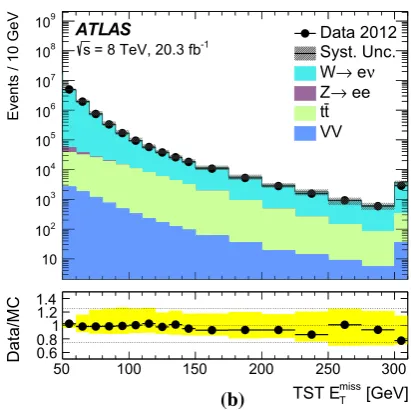
The CST and TSTE_Tmissdistributions inW →eνevents are shown in Fig.6. TheW → τν contributions are com-bined withW → eνevents in the figure. The data and MC simulation agree within the assigned systematic uncertain-ties for both the CST and TST E_Tmissalgorithms. The other E_Tmissalgorithms show similar levels of agreement between data and MC simulation.

6 Performance of the Emiss_T in data and MC simulation

6.1 Resolution ofE_Tmiss

Events / 10 GeV

10 2 10

3 10

4 10

5 10

6 10

7 10

8 10

9 10

Data 2012 Syst. Unc.

ν

e

→

W ee

→

Z t t VV ATLAS

-1 = 8 TeV, 20.3 fb s

[GeV]

miss T

CST E

50 100 150 200 250 300

Data/MC 0.60.8 1 1.2 1.4

Events / 10 GeV

10 2 10

3 10

4 10

5 10

6 10

7 10

8 10

9 10

Data 2012 Syst. Unc.

ν

e

→

W ee

→

Z t t VV ATLAS

-1 = 8 TeV, 20.3 fb s

[GeV]

miss T

TST E

50 100 150 200 250 300

Data/MC 0.60.8 1 1.2 1.4

(a) (b)

Fig. 6 Distributions of theaCST andbTSTEmiss_T as measured in a data sample ofW →eνevents. Thelower panelof the figures show the ratio of data to MC simulation, and thebandscorrespond to the

combined systematic and MC statistical uncertainties. The far right bin includes the integral of all events withE_Tmissabove 300 GeV

The previous ATLASEmiss_T performance paper [1] studied the resolution defined by the width of Gaussian fits in a nar-row range of±2RMS around the mean and used a separate study to investigate the tails. Therefore, the results of this paper are not directly comparable to those of the previous study. The resolutions presented in this paper are expected to be larger than the width of the Gaussian fitted in this manner because the RMS takes into account the tails.

In this section, the resolution for theE_Tmissis presented for Z → μμ events using both data and MC simulation. Unless it is a simulation-only figure (labelled with “Simula-tion” under the ATLAS label), the MC distribution includes the signal sample (e.g. Z→μμ) as well as diboson,tt¯, and t W samples.

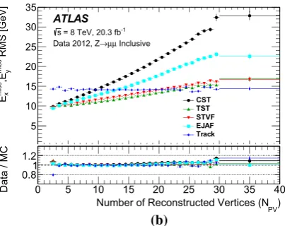
6.1.1 Resolution of the E_Tmissas a function of the number of reconstructed vertices

The stability of theE_Tmissperformance as a function of the amount of pileup is estimated by studying theE_Tmiss reso-lution as a function of the number of reconstructed vertices (NPV) for Z→μμevents as shown in Fig.7. The bin edge is always including the lower edge and not the upper. For example, the events withNPVin the inclusive range 30–39 are combined because of small sample size. In addition, very few events were collected belowNPVof 2 during 2012 data taking. Events in which there are no reconstructed jets with pT>20 GeV are referred to collectively as the 0-jet sample. Distributions are shown here for both the 0-jet and inclusive samples. For both samples, the data and MC simulation agree within 2% up to aroundNPV=15 but the deviation grows

to around 5–10% for NPV>25, which might be attributed to the decreasing sample size. All of the Emiss_T distributions show a similar level of agreement between data and simula-tion across the full range ofNPV.

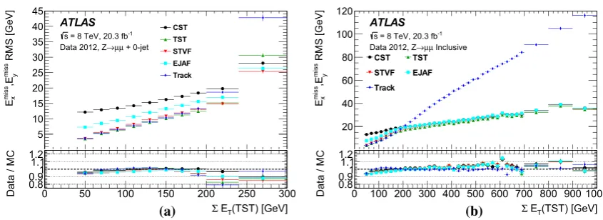
For the 0-jet sample in Fig.7a, the STVF, TST, and Track E_Tmissresolutions all have a small slope with respect toNPV, which implies stability of the resolution against pileup. In addition, their resolutions agree within 1 GeV throughout the NPVrange. In the 0-jet sample, the TST and TrackE_Tmissare both primarily reconstructed from tracks; however, small dif-ferences arise mostly from accounting for photons in the TST E_Tmiss reconstruction algorithm. The CST E_Tmissis directly affected by the pileup as its reconstruction does not apply any pileup suppression techniques. Therefore, the CSTE_Tmisshas the largest dependence on NPV, with a resolution ranging from 7 GeV at NPV =2 to around 23 GeV at NPV =25. The E_Tmissresolution of the EJAF distribution, while better than that of the CSTE_Tmiss, is not as good as that of the other pileup-suppressing algorithms.

For the inclusive sample in Fig. 7b, the Track E_Tmiss is the most stable with respect to pileup with almost no depen-dence on NPV. ForNPV>20, the TrackE_Tmisshas the best resolution showing that pileup creates a larger degradation in the resolution of the otherE_Tmissdistributions than exclud-ing neutral particles, as the TrackE_Tmissalgorithm does. The EJAFEmiss_T algorithm does not reduce the pileup dependence as much as the TST and STVFE_Tmissalgorithms, and the CST E_Tmissagain has the largest dependence onNPV.