This is a repository copy of An Estimate of Equilibrium Climate Sensitivity From Interannual Variability.
White Rose Research Online URL for this paper: http://eprints.whiterose.ac.uk/137128/
Version: Accepted Version
Article:
Dessler, AE and Forster, PM orcid.org/0000-0002-6078-0171 (2018) An Estimate of Equilibrium Climate Sensitivity From Interannual Variability. Journal of Geophysical Research: Atmospheres, 123 (16). pp. 8634-8645. ISSN 2169-897X
https://doi.org/10.1029/2018JD028481
© 2018, American Geophysical Union. All Rights Reserved. This is an author produced version of a paper published in Journal of Geophysical Research: Atmospheres. Uploaded in accordance with the publisher's self-archiving policy.
[email protected] https://eprints.whiterose.ac.uk/ Reuse
Items deposited in White Rose Research Online are protected by copyright, with all rights reserved unless indicated otherwise. They may be downloaded and/or printed for private study, or other acts as permitted by national copyright laws. The publisher or other rights holders may allow further reproduction and re-use of the full text version. This is indicated by the licence information on the White Rose Research Online record for the item.
Takedown
If you consider content in White Rose Research Online to be in breach of UK law, please notify us by
An estimate of equilibrium climate sensitivity from
1
interannual variability
2 3
A.E. Dessler
1*, P.M. Forster
24 5
1 Dept. of Atmospheric Sciences, Texas A&M University. [email protected]
6
2 School of Earth and Environment, University of Leeds, UK [email protected]
7 8 9 10
Main points: 11
1.! We use interannual variability to estimate equilibrium climate sensitivity (ECS). We 12
estimate ECS is likely 2.4-4.6 K (17-83% confidence interval), with a mode and median 13
value of 2.9 and 3.3 K, respectively. 14
2.! We see no evidence to support low ECS (values less than 2K) suggested by other 15
analyses. 16
3.! This work shows the value of alternate energy balance frameworks for understanding 17
climate change. 18
Abstract
20
Estimating the equilibrium climate sensitivity (ECS; the equilibrium warming in response to a
21
doubling of CO2) from observations is one of the big problems in climate science. Using
22
observations of interannual climate variations covering the period 2000 to 2017 and a
model-23
derived relationship between interannual variations and forced climate change, we estimate
24
ECS is likely 2.4-4.6 K (17-83% confidence interval), with a mode and median value of 2.9 and
25
3.3 K, respectively. This analysis provides no support for low values of ECS (below 2 K)
26
suggested by other analyses. The main uncertainty in our estimate is not observational
27
uncertainty, but rather uncertainty in converting observations of short-term, mainly unforced
28
climate variability to an estimate of the response of the climate system to long-term forced
29
warming.
30
Plain language summary
31
Equilibrium climate sensitivity (ECS) is the amount of warming resulting from doubling carbon
32
dioxide. It is one of the important metrics in climate science because it is a primary determinant
33
of how much warming we will experience in the future. Despite decades of work, this quantity
34
remains uncertain: the last IPCC report stated a range for ECS of 1.5-4.5 deg. Celsius. Using
35
observations of interannual climate variations covering the period 2000 to 2017, we estimate
36
ECS is likely 2.4-4.6 K. Thus, our analysis provides no support for the bottom of the IPCC's
37
range.
38
Introduction
40
The response of the climate system to the imposition of a climate forcing is frequently
41
described using the linearized energy balance equation:
42
R = F + l Ts (1)
43
where forcing F is an imposed top-of-atmosphere (TOA) energy imbalance, TS is the global
44
average surface temperature, and l is the change in TOA flux per unit change in TS [Sherwood
45
et al., 2014]. R is the resulting TOA flux imbalance from the combined forcing and response. All
46
quantities are anomalies, i.e., departures from a base state. Equilibrium climate sensitivity
47
(hereafter ECS, the equilibrium warming in response to a doubling of CO2) can be calculated as:
48
ECS = -F2xCO2/l (2)
49
where F2xCO2 is the forcing from doubled CO2.
50
Equation 1 is a workhorse of climate science and it has been used many times to estimate l and
51
ECS. Many of these [e.g., Gregory et al., 2002; Annan and Hargreaves, 2006; Otto et al., 2013;
52
Lewis and Curry, 2015; Aldrin et al., 2012; Skeie et al., 2014; Forster, 2016] combine Eq. 1 with
53
estimates of R, F, and Ts over the 19th and 20th centuries to infer l and ECS. These calculations
54
suggest l is near -2 W/m2/K and appear to rule out an ECS larger than ~4 K [Stevens et al.,
55
2016]. The increased likelihood of an ECS below 2 K implied by these calculations led the IPCC
56
Fifth Assessment Report (AR5) to extend their likely ECS range downward to include 1.5 K
57
[Collins et al., 2013].
58
However, since AR5 a number of problems with this approach have been identified. These
59
include questions about the impact of internal variability [e.g., Dessler et al., 2018], arguments
60
that ECS inferred from historical energy budget produces an underestimate of the true value
61
[e.g., Armour, 2017; Gregory and Andrews, 2016; Zhou et al., 2016; Andrews and Webb, 2018;
62
Proistosescu and Huybers, 2017; Marvel et al., 2018], the large and evolving uncertainty in
63
forcing over the 20th century [e.g., Forster, 2016], different forcing efficacies of greenhouse
64
gases and aerosols [Shindell, 2014; Kummer and Dessler, 2014], and geographically incomplete
65
or inhomogeneous observations [Richardson et al., 2016].
For robust estimates of ECS, multiple lines of evidence are needed and care needs to be taken
67
in relating the inferred ECS from any method to other estimates. Thus, there is great value in
68
finding alternate ways to approach the problem. Relatively few papers have attempted use
69
short-term interannual variability to estimate ECS [e.g., Forster, 2016; Tsushima et al., 2005;
70
Forster and Gregory, 2006; Chung et al., 2010; Tsushima and Manabe, 2013; Dessler, 2013;
71
Donohoe et al., 2014]. Papers that do typically yield estimates of ECS consistent with the IPCC’s
72
canonical ECS range of 1.5-4.5°C, but their uncertainty is so large as to provide no meaningful
73
constraint of the range. In this paper, we present a new methodology that uses interannual
74
fluctuations to help constrain the ECS range.
75
Results 76
Traditional energy-balance framework
77
Per Eq. 2, ECS requires estimates of F2xCO2 and l. We use estimates of F2xCO2 from fixed sea
78
surface temperature and sea-ice experiments from ten global climate models that submitted
79
output to the Precipitation Driver Response Model Intercomparison Project [Myhre et al.,
80
2017b]. They estimate F2xCO2 to be normally distributed with a mean of 3.69 W/m2 and a
81
standard deviation of 0.13 W/m2.
82
We estimate l from observations of R and TS. Observations of R come from the Clouds and the
83
Earth’s Radiant Energy System (CERES) Energy Balanced and Filled product (ed. 4) [Loeb et al.,
84
2018] and cover the period March 2000 to July 2017. Estimates of TS come from the European
85
Centre for Medium Range Weather Forecasts (ECMWF) Interim Re-Analysis (ERAi) [Dee et al.,
86
2011]. In these calculations, monthly and globally averaged anomalies are used, where
87
anomalies are deviations from the mean annual cycle of the data.
88
Given these data, we calculate l two ways, both based on Eq. 1. First, we use estimates of
89
effective radiative forcing F over the CERES period and calculate l as the slope of the regression
90
of R-F vs. TS. We use standard regressions in this paper — an ordinary least-squares fit, with R-F
91
as the dependent variable and TS as the independent variable [Murphy et al., 2009]. The
92
forcing is based on the IPCC AR5 forcing time series, revised and extended in the following
ways. Forcing from CO2, N2O and CH4 have been replaced by calculating new forcing timeseries
94
using concentrations from NOAA/ESRL (www.esrl.noaa.gov/gmd/ccgg/trends/) with updated
95
formula to convert mixing ratios to forcing [Etminan et al., 2016]. Other forcing components
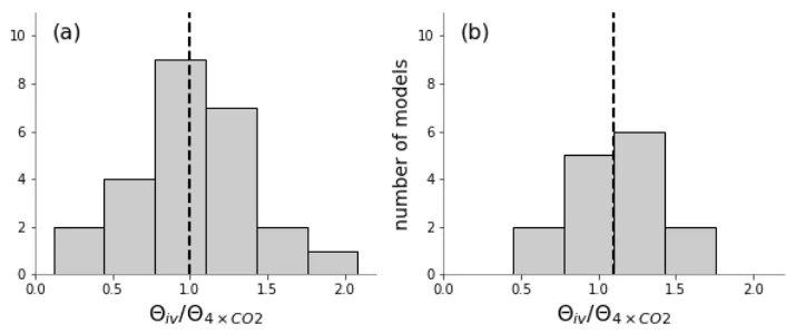
96
match IPCC AR5 through 2011 and have been extended to July 2017. For aerosols and ozone,
97
the multi-model mean forcing from Myhre et al. [2017a] is used. For volcanoes, the forcing
98
from Andersson et al. [2015] is taken from their Figure 4, beginning in 2008. Solar forcing after
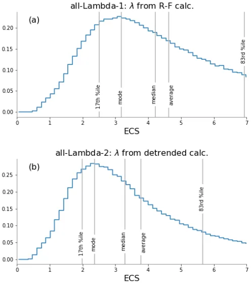
99
2011 is derived from SORCE data [Lean et al., 2005]. Other minor forcing terms are estimated
100
using the relative change in forcing from 2011-2017 from the RCP4.5 scenario [Meinshausen et
101
al., 2011].
102
Uncertainty is estimated using radiative forcing uncertainties from 2015. We take the 5%-95%
103
range for each of the 14 different forcing terms in 2015 and turn this into a fractional range by
104
dividing by the median 1750-2015 forcing estimate. This fractional uncertainty is Monte Carlo
105
sampled for each forcing term independently. These fractions are then multiplied by the
106
relevant forcing time series and summed to create 10,000 different realizations of the time
107
series of total radiative forcing. The average forcing time series during the CERES period is
108
plotted in Fig. S1.
109
We then estimate a distribution of l using Monte Carlo sampling. We start by subtracting the
110
10,000 forcing time series from the observed R time series to generate 10,000 estimates of R-F.
111
Then we repeat the following process 500,000 times: 1) randomly select an R-F time series, 2)
112
randomly subsample it and the observed TS time series, with replacement, 3) regress the
113
sampled R-F and TS data sets to obtain an estimate of l. The number of samples taken is set by
114
the number of independent pieces of information in the time series, as estimated by Eq. 6 of
115
Santer et al. [2000] (the original data set contains 209 months; we estimate there are ~100-120
116
independent samples due to autocorrelation in the time series).
117
In the second approach, we assume forcing changes linearly over the CERES time period and
118
account for it by detrending R and TS time series. We do this by subtracting off the linear trend
119
of each time series estimated using a least-squares regression. We then assume that
120
Rdetrended = l TS,detrended and we calculate l by regression. The distribution of l is estimated by
randomly sampling 500,000 times (with replacement) the detrended R and TS time series, with
122
each resampled data set providing one estimate l. As with the previous estimate, we account
123
for autocorrelation by reducing the number of samples taken, using Eq. 6 of Santer et al.
124
[2000]. Plots of R, TS, and F can be found in Section S1 of the supplement.
125
Distributions of l for the two approaches are both quite wide (Fig. 1a), with values of
126
-0.51±0.64 and -0.81±0.65 W/m2/K for the R-F and detrended calculations, respectively
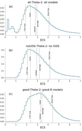
127
(uncertainties are 5-95% confidence intervals). The two estimates of l reflect different ways of
128
handing forcing and they show that different approaches yield similar distributions for l. These
129
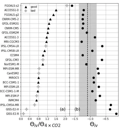
distributions are similar to those estimated as the uncertainty of ordinary least-squares
130
regressions of R-F vs. TS (-0.52±0.56 W/m2) and detrended R vs. detrended TS (-0.82±0.64
131
W/m2). Our sign convention is that fluxes are downward positive, so a negative l means that a
132
warmer planet radiates more energy to space, a necessary requirement for a stable climate.
133
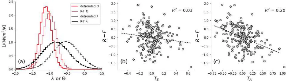
The extreme width of the l distributions is a consequence of scatter in the relationship
134
between R-F and TS (Fig. 1b) [Spencer and Braswell, 2010; Xie et al., 2016], which is due to both
135
weak coupling between the surface and ∆R [Dessler et al., 2018] and weather noise. This
136
means that our observational estimate of l is quite uncertain, with almost all of the uncertainty
137
coming from month-to-month variability in the R time series. Switching to another
138
temperature data set, such as MERRA2 [Gelaro et al., 2017], or using only the median forcing,
139
yields very similar distributions. Systematic errors in the CERES time series are small; the data
140
are stable to better than 0.5 W/m2/decade (stability of the shortwave is 0.3 W/m2/decade
141
[Loeb et al., 2007], and longwave is 0.15 W/m2/decade [Susskind et al., 2012]). Because we are
142
regressing R vs. temperature, spurious trends in the data have little impact on our analysis
143
[Dessler, 2010].
144
The distributions of l plotted in Fig. 1a are derived mainly from the response to interannual
145
variability (Fig. S3), so we will refer to them hereafter as liv. The l in Eq. 2, however, is the
146
climate system’s response to forcing from doubled CO2 (hereafter l2xCO2), so we cannot simply
147
plug liv into Eq. 2 to derive ECS. In fact, this disconnect between what we can measure (liv)
and what is required to calculate ECS (l2xCO2) is one reason scientists have largely avoided using
149
interannual variability to infer ECS.
150
We therefore modify Eq. 2 to account for this:
151
ECS= −&∋×CO2
+,−,/01
+,− +∋×23∋
(3)
152
where liv,obs is the observed value (from Fig. 1a), mainly the response to interannual variability,
153
while the ratio liv/l2xCO2 is a transfer function that converts liv,obs into the required value l2xCO2.
154
We estimate this transfer function using models that submitted required output to the 5th
155
phase of the Coupled Model Intercomparison Project (CMIP5) [Taylor et al., 2012]. The
156
numerator liv is derived from the models’ control runs, in which climate variations arise
157
naturally from internal variability. To facilitate comparison with the observations, as well as
158
avoid any issues with long-term drift, we first break each control run into 16-year segments and
159
calculate monthly anomalies of ∆R and ∆TS during each segment, where anomalies are
160
deviations from the average annual cycle of each 16-year period. We expect these model
161
segments to contain the same types of climate variations that are in the observations (e.g.,
162
weather noise, ENSO). Then, we calculate liv for each segment as the slope of the regression of
163
∆R vs. ∆TS for that segment. Finally, we average the segments’ values of liv to come up with a
164
single value of liv for each model (Table S1).
165
The CMIP5 archive does not include doubled CO2 runs, but it does have abrupt 4xCO2 runs from
166
which we can estimate l4xCO2. l4xCO2 is calculated from these runs using the Gregory et al.
167
[Gregory et al., 2004] method: we regress all 150 years of annual R vs. annual average TS, and
168
take the resulting slope as an estimate of l4xCO2, where R and TS are deviations from the
pre-169
industrial control run.
170
If we assume that l2xCO2 ≈ l4xCO2, so we can re-write Eq. 3 as:
171
ECS≈ −&∋×CO2
+,−,/01
+,− +5×23∋
(4)
Recent work suggests that l4xCO2 is less negative (i.e., implying a higher ECS) than l2xCO2
173
[Armour, 2017; Proistosescu and Huybers, 2017]. On the other hand, we use all 150 years of the
174
4xCO2 runs to estimate l4xCO2, which tends to produce values that are too negative [Andrews et
175
al., 2015; Rugenstein et al., 2016; Rose and Rayborn, 2016; Armour, 2017]. These two errors
176
tend to cancel, but how much of a bias is left — and in which direction — remains an
177
uncertainty in this analysis. The CMIP5 ensemble’s distribution of liv/l4xCO2 is plotted in Fig. 2;
178
it has an average of 0.81 and a standard deviation of 0.34.
179
We then use a Monte Carlo approach to estimate ECS. We produce 500,000 estimates of ECS
180
by randomly sampling the distributions of F2xCO2, liv,obs (Fig. 1a), and liv/l4xCO2 (Fig. 2) and
181
plugging them into Eq. 3; negative ECS values or values greater than 10 K are viewed as
182
physically implausible and thrown out (sensitivity to the 10-K threshold is shown in Table 1). We
183
produce two ECS distributions — one using liv,obs from the R-F calculation and one using liv,obs
184
from the detrended calculation. The ECS distributions (Fig. 3) have 17-83% confidence intervals
185
(corresponding to the IPCC’s likely range) of 2.5-7.0 K and 2.0-5.7 K for the R-F and detrended
186
calculations, respectively. The modes are 3.0 and 2.4 K, while the medians are 4.2 and 3.3 K.
187
Overall, our calculated ECS distributions overlap substantially with the IPCC’s range, although
188
our distributions are shifted to higher values: we see a ~30% chance that ECS exceeds 4.5 K,
189
while the IPCC assigns that a 17% chance. And we see less support for low values of ECS: the
190
chance of an ECS below 2 K is 6-15%, while the IPCC assigns a 17% chance it is below 1.5 K.
191
Table 1 lists the statistics of these distributions, as well as a number of sensitivity tests to
192
determine the robustness of the calculation. For example, we have done ECS calculations using
193
a F2xCO2 distribution derived from the CMIP5 abrupt 4xCO2 runs instead of the distribution from
194
the PDRMIP (see Sect. S2 for more about this). All of the ECS distributions are similar to those
195
shown in Fig. 3, leading us to conclude that our conclusions are robust with respect to the many
196
choices in how the calculation is done.
197
Modified energy-balance framework
Recently, Dessler et al. [2018] suggested a revision of Eq. 1, where the TOA flux is
199
parameterized in terms of tropical atmospheric temperature, not global surface temperature:
200
R = F + Q TA (5)
201
where TA is the tropical average (30°N-30°S) 500-hPa temperature and Q converts this quantity
202
to TOA flux. R and F are the same global average quantities they were in equation 1. They
203
demonstrated that TA correlated better with R-F than TS does (Fig. 1c), thereby providing a
204
superior way to describe global energy balance.
205
In this framework, the equilibrium warming of the tropical atmosphere ∆TA in response to
206
doubled CO2 is equal to -F2xCO2/Q2xCO2. ECS can therefore be written
207
ECS= −&∋×CO2
6,−,/01 6,−
6∋×23∋
789
78:
≈ −&∋×CO2
6,−,/01 6,− 65×23∋ 789 78: (6) 208
where Qiv,obs is the analog to liv,obs, Qiv/Q2xCO2 is the transfer function that allows us to use
209
short-term variability to estimate ECS, and ∆TS/∆TA is the ratio of the temperature changes at
210
equilibrium in response to doubled CO2. As we did previously, we will further assume that
211
Q4xCO2 ≈ Q2xCO2.
212
We use the same forcing F2xCO2 that was used in the previous section. The distributions of the
213
scaling factor Qiv/Q4xCO2 (Fig. 4a) come from the CMIP5 ensemble. These are calculated the
214
same way as the liv/l4xCO2 ratios were, except atmospheric temperatures are substituted for
215
surface temperatures. Just as we did for liv,obs, we calculate Qiv,obs two ways: by regressing R-F
216
vs. TA and by regressing detrended R vs. detrended TA . Distributions of Qiv,obs for the two
217
approaches are similar (Fig. 1a), with values of -0.98±0.32 and -1.09±0.29 W/m2/K for the R-F
218
and detrended calculations, respectively (uncertainties are 5-95% confidence intervals).
219
Because of their similarities, in the rest of this section we will show results using the detrended
220
calculation, although results for both distributions can be found in Table 2.
221
Finally, the distribution of the temperature ratio ∆TS/∆TA is also estimated from the CMIP5
222
ensemble. For each model, ∆TS and ∆TA are estimated as the average difference of the first and
last decades of the abrupt 4xCO2 runs; we then take the ratio of these values. Comparisons of
224
the models to observations show that models do well at simulating this ratio (Sect. S3). The
225
resulting distribution of ∆TS/∆TA constructed by the CMIP5 models (Fig. 5a) has an ensemble
226
average and standard deviation of 0.86±0.10.
227
Long forced runs of the MPI-ESM1.1, GFDL CM3, and ESM2M models all show this ratio
228
increases as the climate continues to warm beyond year 150. In runs of the GFDL CM3 and
229
ESM2M, in which CO2 increases at 1% per year until doubling and then remains fixed, the ratio
230
increases from 0.79 and 0.70, 300 years after CO2 doubles, to 0.86 and 0.76 at equilibrium
231
(GFDL values are personal communication, David Paynter, 2018, based on runs described in
232
[Paynter et al., 2018]). The ratio in an abrupt 4xCO2 run of the MPI model increases from 0.79
233
in years 140-150 to 0.87 in years 2400-2500. Thus, we conclude that values of this ratio
234
obtained from the 150-year CMIP5 4xCO2 simulations may be low biased, which would lead our
235
ECS to also be low biased.
236
As in the previous section, we use a Monte Carlo approach and produce 500,000 estimates of
237
ECS by randomly sampling the distributions of F2xCO2, Qiv,obs, Qiv/Q4xCO2, and ∆TS/∆TA, and then
238
plugging the values into Eq. 6. The resulting ECS distribution (Fig. 6a) shows a similar structure
239
to the l-based distributions in Fig. 3: a broad maximum between 2 and 3 K and a tail towards
240
higher ECS values.
241
There is also a puzzling peak below 1°C. The only way for an ECS estimate to be close to zero is
242
if Qiv,obs is very large or one of the other factors in Eq. 6 is close to zero. Analysis of the terms in
243
Eq. 6 suggests that the term causing the low ECS values is Qiv/Q4xCO2, whose distribution
244
approaches zero (Fig. 4a). These low values come from the GISS models (Fig. 7a, Table S1) and if
245
they are removed from the ensemble, the bump below 1 K disappears (Fig. 6b), although the
246
statistics of the distribution do not change much.
247
This result emphasizes that the scaling factor Qiv/Q4xCO2 is unconstrained by observations and
248
has not been previously studied. That doesn’t mean, however, that we know nothing about it
249
— we do have observations of Qiv and can compare those to each model’s value of Qiv. We find
that 15 of the 25 CMIP5 models produce estimates of Qiv in agreement with the CERES
251
observations (Fig. 7b). If we construct distributions of Qiv/Q4xCO2 and ∆TS/∆TA from just those
252
models (Figs. 4b and 5b), we obtain the ECS distribution in Fig. 6c (hereafter referred to as the
253
“good-Q” distribution).
254
We consider the “good-Q” ECS distributions to be the best estimates of ECS from this analysis.
255
Those ECS distributions have 17-83% confidence intervals (corresponding to the IPCC’s likely
256
range) of 2.4-4.7 K and 2.4-4.4 K for the R-F and detrended calculations, respectively. Averaging
257
these gives us our single best estimate for the likely range, 2.4-4.6 K, and 5-95% range, 1.9-5.7
258
K. The modes are 2.6 and 3.1 K (average 2.9 K), and the medians of both are 3.3 K.
259
These distributions suggest a 15-20% chance ECS exceeds 4.5 K and a 6% chance of an ECS
260
below 2 K. We therefore conclude that the IPCC’s upper end of the likely ECS range is about
261
right, but that the low end is too low. We would conclude that, in the parlance of the IPCC, ECS
262
is very unlikely to be below 2 K.
263
We have also performed corresponding “good-l” ECS calculations in which the liv/l4xCO2
264
distribution in Eq. 4 is constructed using only those models whose liv agrees with liv,obs. The
265
ECS distributions obtained from these calculations (Table 1) are similar to distributions from the
266
l calculations using all models.
267
Discussion
268
There are several reasons why ECS estimated from the revised energy balance framework (Eq.
269
6) should be considered more reliable than that estimated from the traditional framework (Eq.
270
4) used in previous papers [e.g., Forster, 2016; Tsushima et al., 2005; Forster and Gregory,
271
2006; Chung et al., 2010; Tsushima and Manabe, 2013; Dessler, 2013; Donohoe et al., 2014].
272
Fig. 1 shows the main advantage — that Qiv,obs is better constrained than liv,obs This is what
273
leads to the narrower distributions of ECS in Fig. 6 than in Fig. 3. Of particular note, the liv,obs
274
distributions have non-zero probabilities of values close to zero; since ECS is proportional to
275
1/liv,obs, this generates a large tail towards unrealistically large ECS values.
There are additional reasons that lead us to conclude that the estimates from the revised
277
framework are superior. It has been suggested that liv,obs exhibits significant decadal variability
278
in models [Andrews et al., 2015; Gregory and Andrews, 2016; Zhou et al., 2016; Dessler et al.,
279
2018]. This opens the possibility that the observed liv,obs, based on 16 years of data, is biased
280
with respect to the long-term average; if so, then ECS estimated from these observations would
281
also be biased. Model simulations suggest that Qiv,obs exhibits smaller decadal variability
282
[Dessler et al., 2018], making Qiv estimated from CERES data a more robust estimate of the
283
climate system’s actual long-term value. There is also evidence that Q changes less than l
284
during transient climate change [Dessler et al., 2018], making the assumption that Q2xCO2 ≈
285
Q4xCO2 a far better one than the assumption that l4xCO2 ≈ l2xCO2.
286
It is also worth stepping back and asking what could cause our calculation to be seriously in
287
error. It seems unlikely that forcing from doubled CO2 is wrong given our good understanding
288
of the physics of CO2 forcing [e.g., Feldman et al., 2015]. Estimates of liv,obs and Qiv,obs are
289
derived from observations we view to be reliable, so our judgment is that they are also unlikely
290
to be significantly wrong. The ∆TS/∆TA factor comes from climate model simulations, but
291
models have long been able to accurately reproduce the observed pattern of surface warming
292
[e.g., Stouffer and Manabe, 2017], and we have simple physical arguments explaining how the
293
atmospheric and surface temperature should be connected [Xu and Emanuel, 1989]. Finally,
294
we can compare the models to data [Compo et al., 2011; Poli et al., 2016] to validate their
295
simulation of this ratio (Sect. S3).
296
Thus, the transfer function Qiv/Q4xCO2 seems the most probable place for a significant error to
297
occur. That said, there are reasons to believe the models’ estimates of this ratio. As mentioned
298
above, we can directly compare Qiv in the models to observations, and find agreement in the
299
majority of models (Fig. 7). We also argue that while errors may exist in a model (i.e., in the
300
cloud feedback), this will affect both the numerator and denominator and such errors will tend
301
to cancel out. As a preliminary test of this, we have analyzed three different versions of the
302
MPI-ESM 1.2 model that have had their cloud feedbacks modified to produce different ECS
303
[Thorsten Mauritsen and Diego Jimenez, personal communication, 2018]. The three versions
are the standard model (ECS calculated from an abrupt 4xCO2 run using the Gregory method =
305
3.0 K), an “iris” version [described in Mauritsen and Stevens, 2015] (ECS = 2.6 K), and a “high
306
ECS” version, in which the convective parameterization has been tweaked to generate a large,
307
positive cloud feedback (ECS = 5.2 K). Despite large differences in the ECS, these three versions
308
have similar values of liv/l4xCO2 of 1.17, 1.15, and 1.11 for the standard, iris, and high ECS
309
versions, respectively. The corresponding values of Qiv/Q4xCO2 are 1.06, 0.96, and 1.10. While
310
one must be careful about conclusions based on a single model, this nevertheless provides
311
some support for the hypothesis that errors in Q4xCO2 will cancel errors in Qiv when the ratio is
312
taken and that the ratio Q4xCO2/Qiv may well be more accurate than either Q4xCO2 or Qiv are
313
individually.
314
We have also constructed an error budget to determine which term contributes most to the
315
width of the distributions in Fig. 6. We do this by sequentially setting each term to have zero
316
uncertainty by replacing that term’s distribution in the Monte Carlo calculation with a single
317
number, the ensemble average. This has little effect on the mean, median, or mode, but does
318
change the width of the distribution (Table 3). By comparing the widths of the resulting
319
distributions (defined as the distance between the 17th and 83rd percentiles), Fig. 8 shows that
320
the biggest contributor to ECS uncertainty is the uncertainty in Qiv/Q4xCO2. Eliminating the
321
uncertainty in that reduces the 17-83% confidence interval to 2.8-4.0 K. Thus, developing a
322
theoretical argument for the value of this ratio would be a key advance in climate science. The
323
next most important uncertainty is uncertainty in Qiv,obs, followed by the uncertainty in ∆TS/∆TA
324
and then the uncertainty in F2xCO2.
325
Conclusions
326
Estimating ECS from observations remains one of the big problems in climate science. Despite
327
several decades of intense investigations, the uncertainty in this parameter remains stubbornly
328
large, with the last IPCC assessment reporting a likely range of 1.5-4.5 K (17-83% confidence
329
interval). Because of this, there is great value in finding alternate ways to approach the
330
problem.
In this paper, we have used observations of interannual climate variations covering the period
332
2000 to 2017 along with a model-derived relationship between interannual variations and
333
forced climate change to estimate ECS. We interpret the observations using a modified energy
334
balance framework (Eq. 5) in which the response of TOA flux is proportional to the atmospheric
335
temperature. We conclude ECS is likely 2.4-4.6 K (17-83% confidence interval), with a mode and
336
median value of 2.9 and 3.3 K, respectively. Overall, our analysis suggests that the upper end of
337
the IPCC’s range is set about right, but this analysis provides little evidence to support estimates
338
of ECS in the bottom third of the IPCC’s likely range.
339
One of the key parts of our calculations is the use of CMIP5 climate models to convert the
340
observations of interannual variability into an estimate of the response of the system to
341
doubled CO2. This is the main uncertainty in our analysis and future efforts to pin this transfer
342
function down would be extremely valuable.
343
References
344
Aldrin, M., M. Holden, P. Guttorp, R. B. Skeie, G. Myhre, & T. K. Berntsen (2012), Bayesian 345
estimation of climate sensitivity based on a simple climate model fitted to observations of 346
hemispheric temperatures and global ocean heat content, Environmetrics, 23, 253-271, doi: 347
10.1002/env.2140. 348
Andersson, S. M., B. G. Martinsson, J.-P. Vernier, J. Friberg, C. A. M. Brenninkmeijer, M. 349
Hermann, et al. (2015), Significant radiative impact of volcanic aerosol in the lowermost 350
stratosphere, Nature Communications, 6, 7692, doi: 10.1038/ncomms8692. 351
Andrews, T., & M. J. Webb (2018), The dependence of global cloud and lapse rate feedbacks on 352
the spatial structure of tropical Pacific warming, J. Climate, 31, 641-654, doi: 10.1175/jcli-353
d-17-0087.1. 354
Andrews, T., J. M. Gregory, & M. J. Webb (2015), The dependence of radiative forcing and 355
feedback on evolving patterns of surface temperature change in climate models, J. Climate, 356
28, 1630-1648, doi: 10.1175/JCLI-D-14-00545.1. 357
Annan, J. D., & J. C. Hargreaves (2006), Using multiple observationally-based constraints to 358
estimate climate sensitivity, Geophys. Res. Lett., 33, doi: 10.1029/2005gl025259. 359
Armour, K. C. (2017), Energy budget constraints on climate sensitivity in light of inconstant 360
climate feedbacks, Nature Clim. Change, 7, 331-335, doi: 10.1038/nclimate3278. 361
Chung, E. S., B. J. Soden, & B. J. Sohn (2010), Revisiting the determination of climate 362
sensitivity from relationships between surface temperature and radiative fluxes, Geophys. 363
Collins, M., R. Knutti, J. Arblaster, J.-L. Dufresne, T. Fichefet, P. Friedlingstein, et al. (2013), 365
Long-term climate change: Projections, commitments and irreversibility, in Climate Change 366
2013: The Physical Science Basis. Contribution of Working Group I to the Fifth Assessment 367
Report of the Intergovernmental Panel on Climate Change, edited by T. F. Stocker, D. Qin, 368
G.-K. Plattner, M. Tignor, S. K. Allen, J. Boschung, A. Nauels, Y. Xia, V. Bex and P. M. 369
Midgley, Cambridge University Press, Cambridge, United Kingdom and New York, NY, 370
USA. 371
Compo, G. P., J. S. Whitaker, P. D. Sardeshmukh, N. Matsui, R. J. Allan, X. Yin, et al. (2011), 372
The Twentieth Century Reanalysis Project, Q. J. R. Meteor. Soc., 137, 1-28, doi: 373
10.1002/qj.776. 374
Dee, D. P., S. M. Uppala, A. J. Simmons, P. Berrisford, P. Poli, S. Kobayashi, et al. (2011), The 375
ERA-Interim reanalysis: Configuration and performance of the data assimilation system, Q. 376
J. R. Meteor. Soc., 137, 553-597, doi: 10.1002/qj.828. 377
Dessler, A. E. (2010), A Determination of the Cloud Feedback from Climate Variations over the 378
Past Decade, Science, 330, 1523-1527, doi: 10.1126/science.1192546. 379
Dessler, A. E. (2013), Observations of climate feedbacks over 2000-10 and comparisons to 380
climate models, J. Climate, 26, 333-342, doi: 10.1175/jcli-d-11-00640.1. 381
Dessler, A. E., T. Mauritsen, & B. Stevens (2018), The influence of internal variability on Earth's 382
energy balance framework and implications for estimating climate sensitivity, Atmos. 383
Chem. Phys., 18, 5147-5155, doi: 10.5194/acp-18-5147-2018. 384
Donohoe, A., K. C. Armour, A. G. Pendergrass, & D. S. Battisti (2014), Shortwave and 385
longwave radiative contributions to global warming under increasing CO2, Proc. Natl. 386
Acad. Sci., 111, 16700-16705, doi: 10.1073/pnas.1412190111. 387
Etminan, M., G. Myhre, E. J. Highwood, & K. P. Shine (2016), Radiative forcing of carbon 388
dioxide, methane, and nitrous oxide: A significant revision of the methane radiative forcing, 389
Geophys. Res. Lett., 43, 12,614-612,623, doi: 10.1002/2016GL071930. 390
Feldman, D. R., W. D. Collins, P. J. Gero, M. S. Torn, E. J. Mlawer, & T. R. Shippert (2015), 391
Observational determination of surface radiative forcing by CO2 from 2000 to 2010, Nature, 392
519, 339, doi: 10.1038/nature14240. 393
Forster, P. M. (2016), Inference of climate sensitivity from analysis of Earth's energy budget, 394
Annual Review of Earth and Planetary Sciences, 44, 85-106, doi: 10.1146/annurev-earth-395
060614-105156. 396
Forster, P. M. D., & J. M. Gregory (2006), The climate sensitivity and its components diagnosed 397
from Earth Radiation Budget data, J. Climate, 19, 39-52. 398
Gelaro, R., W. McCarty, M. J. Su‡rez, R. Todling, A. Molod, L. Takacs, et al. (2017), The 399
Modern-Era Retrospective Analysis for Research and Applications, Version 2 (MERRA-2), 400
J. Climate, 30, 5419-5454, doi: 10.1175/jcli-d-16-0758.1. 401
Gregory, J. M., & T. Andrews (2016), Variation in climate sensitivity and feedback parameters 402
during the historical period, Geophys. Res. Lett., 43, 3911-3920, doi: 403
Gregory, J. M., R. J. Stouffer, S. C. B. Raper, P. A. Stott, & N. A. Rayner (2002), An 405
observationally based estimate of the climate sensitivity, J. Climate, 15, 3117-3121, doi: 406
10.1175/1520-0442(2002)015<3117:aobeot>2.0.co;2. 407
Gregory, J. M., W. J. Ingram, M. A. Palmer, G. S. Jones, P. A. Stott, R. B. Thorpe, et al. (2004), 408
A new method for diagnosing radiative forcing and climate sensitivity, Geophys. Res. Lett., 409
31, doi: 10.1029/2003gl018747. 410
Kummer, J. R., & A. E. Dessler (2014), The impact of forcing efficacy on the equilibrium 411
climate sensitivity, Geophys. Res. Lett., 41, 3565-3568, doi: 10.1002/2014gl060046. 412
Lean, J., G. Rottman, J. Harder, & G. Kopp (2005), SORCE contributions to new understanding 413
of global change and solar variability, Solar Physics, 230, 27-53, doi: 10.1007/s11207-005-414
1527-2. 415
Lewis, N., & J. A. Curry (2015), The implications for climate sensitivity of AR5 forcing and heat 416
uptake estimates, Climate Dynamics, 45, 1009-1023, doi: 10.1007/s00382-014-2342-y. 417
Loeb, N. G., S. Kato, K. Loukachine, N. Manalo-Smith, & D. R. Doelling (2007), Angular 418
distribution models for top-of-atmosphere radiative flux estimation from the Clouds and the 419
Earth's Radiant Energy System instrument on the Terra satellite. Part II: Validation, Journal 420
of Atmospheric and Oceanic Technology, 24, 564-584. 421
Loeb, N. G., D. R. Doelling, H. Wang, W. Su, C. Nguyen, J. G. Corbett, et al. (2018), Clouds 422
and the EarthÕs Radiant Energy System (CERES) Energy Balanced and Filled (EBAF) Top-423
of-Atmosphere (TOA) Edition-4.0 Data Product, J. Climate, 31, 895-918, doi: 10.1175/jcli-424
d-17-0208.1. 425
Marvel, K., R. Pincus, G. A. Schmidt, & R. L. Miller (2018), Internal variability and 426
disequilibrium confound estimates of climate sensitivity from observations, Geophys. Res. 427
Lett., doi: 10.1002/2017GL076468. 428
Mauritsen, T., & B. Stevens (2015), Missing iris effect as a possible cause of muted hydrological 429
change and high climate sensitivity in models, Nature Geosci, 8, 346-351, doi: 430
10.1038/ngeo2414. 431
Meinshausen, M., S. J. Smith, K. Calvin, J. S. Daniel, M. L. T. Kainuma, J.-F. Lamarque, et al. 432
(2011), The RCP greenhouse gas concentrations and their extensions from 1765 to 2300, 433
Climatic Change, 109, 213, doi: 10.1007/s10584-011-0156-z. 434
Murphy, D. M., S. Solomon, R. W. Portmann, K. H. Rosenlof, P. M. Forster, & T. Wong (2009), 435
An observationally based energy balance for the Earth since 1950, J. Geophys. Res., 114, 436
14, doi: 10.1029/2009jd012105. 437
Myhre, G., W. Aas, R. Cherian, W. Collins, G. Faluvegi, M. Flanner, et al. (2017a), Multi-model 438
simulations of aerosol and ozone radiative forcing due to anthropogenic emission changes 439
during the period 1990Ð2015, Atmos. Chem. Phys., 17, 2709-2720, doi: 10.5194/acp-17-440
2709-2017. 441
Myhre, G., P. M. Forster, B. H. Samset, ¯. Hodnebrog, J. Sillmann, S. G. Aalbergsj¿, et al. 442
Protocol and Preliminary Results, Bull. Am. Met. Soc., 98, 1185-1198, doi: 10.1175/bams-444
d-16-0019.1. 445
Otto, A., F. E. L. Otto, O. Boucher, J. Church, G. Hegerl, P. M. Forster, et al. (2013), Energy 446
budget constraints on climate response, Nature Geoscience, 6, 415-416, doi: 447
10.1038/ngeo1836. 448
Paynter, D., T. L. Fršlicher, L. W. Horowitz, & L. G. Silvers (2018), Equilibrium Climate 449
Sensitivity Obtained From Multimillennial Runs of Two GFDL Climate Models, Journal of 450
Geophysical Research: Atmospheres, 123, 1921-1941, doi: doi:10.1002/2017JD027885. 451
Poli, P., H. Hersbach, D. P. Dee, P. Berrisford, A. J. Simmons, F. Vitart, et al. (2016), ERA-20C: 452
An Atmospheric Reanalysis of the Twentieth Century, J. Climate, 29, 4083-4097, doi: 453
10.1175/jcli-d-15-0556.1. 454
Proistosescu, C., & P. J. Huybers (2017), Slow climate mode reconciles historical and model-455
based estimates of climate sensitivity, Science Advances, 3, doi: 10.1126/sciadv.1602821. 456
Richardson, M., K. Cowtan, E. Hawkins, & M. B. Stolpe (2016), Reconciled climate response 457
estimates from climate models and the energy budget of Earth, Nature Clim. Change, 6, 458
931-935, doi: 10.1038/nclimate3066. 459
Rose, B. E. J., & L. Rayborn (2016), The effects of ocean heat uptake on transient climate 460
sensitivity, Current Climate Change Reports, 2, 190-201, doi: 10.1007/s40641-016-0048-4. 461
Rugenstein, M. A. A., K. Caldeira, & R. Knutti (2016), Dependence of global radiative 462
feedbacks on evolving patterns of surface heat fluxes, Geophys. Res. Lett., 43, 9877-9885, 463
doi: 10.1002/2016GL070907. 464
Santer, B. D., T. M. L. Wigley, J. S. Boyle, D. J. Gaffen, J. J. Hnilo, D. Nychka, et al. (2000), 465
Statistical significance of trends and trend differences in layer-average atmospheric 466
temperature time series, J. Geophys. Res., 105, 7337-7356, doi: 10.1029/1999jd901105. 467
Sherwood, S. C., S. Bony, O. Boucher, C. Bretherton, P. M. Forster, J. M. Gregory, & B. Stevens 468
(2014), Adjustments in the forcing-feedback framework for understanding climate change, 469
Bull. Am. Met. Soc., 96, 217-228, doi: 10.1175/BAMS-D-13-00167.1. 470
Shindell, D. T. (2014), Inhomogeneous forcing and transient climate sensitivity, Nature Climate 471
Change, 4, 274, doi: 10.1038/nclimate2136. 472
Skeie, R. B., T. Berntsen, M. Aldrin, M. Holden, & G. Myhre (2014), A lower and more 473
constrained estimate of climate sensitivity using updated observations and detailed radiative 474
forcing time series, Earth System Dynamics, 5, 139-175, doi: 10.5194/esd-5-139-2014. 475
Spencer, R. W., & W. D. Braswell (2010), On the diagnosis of radiative feedback in the presence 476
of unknown radiative forcing, J. Geophys. Res., 115, doi: 10.1029/2009JD013371. 477
Stevens, B., S. C. Sherwood, S. Bony, & M. J. Webb (2016), Prospects for narrowing bounds on 478
Earth's equilibrium climate sensitivity, Earth's Future, 4, 512-522, doi: 479
10.1002/2016EF000376. 480
Stouffer, R. J., & S. Manabe (2017), Assessing temperature pattern projections made in 1989, 481
Susskind, J., G. Molnar, L. Iredell, & N. G. Loeb (2012), Interannual variability of outgoing 483
longwave radiation as observed by AIRS and CERES, J. Geophys. Res., 117, doi: 484
10.1029/2012jd017997. 485
Taylor, K. E., R. J. Stouffer, & G. A. Meehl (2012), An overview of CMIP5 and the experiment 486
design, Bull. Am. Met. Soc., 93, 485-498, doi: 10.1175/bams-d-11-00094.1. 487
Tsushima, Y., & S. Manabe (2013), Assessment of radiative feedback in climate models using 488
satellite observations of annual flux variation, Proc. Natl. Acad. Sci., 110, 7568-7573, doi: 489
10.1073/pnas.1216174110. 490
Tsushima, Y., A. Abe-Ouchi, & S. Manabe (2005), Radiative damping of annual variation in 491
global mean surface temperature: comparison between observed and simulated feedback, 492
Climate Dynamics, 24, 591-597, doi: 10.1007/s00382-005-0002-y. 493
Xie, S.-P., Y. Kosaka, & Y. M. Okumura (2016), Distinct energy budgets for anthropogenic and 494
natural changes during global warming hiatus, Nature Geoscience, 9, 29-33, doi: 495
10.1038/ngeo2581. 496
Xu, K. M., & K. A. Emanuel (1989), Is the tropical atmosphere conditionally unstable?, Mon. 497
Wea. Rev., 117, 1471-1479. 498
Zhou, C., M. D. Zelinka, & S. A. Klein (2016), Impact of decadal cloud variations on the Earth's 499
energy budget, Nature Geosci, 9, 871-874, doi: 10.1038/ngeo2828. 500
501
Acknowledgments: A.E.D. acknowledges support from NSF grant AGS-1661861 to Texas 503
A&M University. P.M.F. acknowledges support from the Natural Environment Research 504
Council project NE/P014844/1. We thank Bjorn Stevens and Thorsten Mauritsen for their 505
insight into this analysis. We also acknowledge the modeling groups, the Program for Climate 506
Model Diagnosis and Intercomparison, and the WCRPÕs Working Group on Coupled Modeling 507
for their roles in making available the WCRP CMIP5 multimodel dataset. CERES data were 508
downloaded from ceres.larc.nasa.gov, CMIP5 data were downloaded from cmip.llnl.gov, and 509
ECMWF reanalysis were downloaded from www.ecmwf.int/en/forecasts/datasets/reanalysis-510
datasets/era-interim. Code and data can be found here: https://zenodo.org/record/1323162. 511
513 514 515
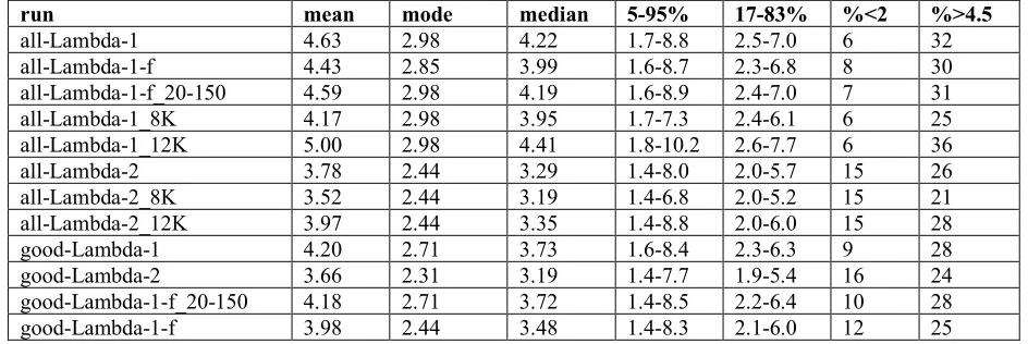
Table 1. ECS values from the l runs
516
Summary of the statistics of the ECS distributions derived using Eq. 4. Ò%<2Ó and Ò%>4.5Ó 517
gives the percent of ECS values that are below 2 K or above 4.5 K. Units are in K, except for 518
Ò%<2Ó and Ò%>4.5Ó, which are in percent. 519
run mean mode median 5-95% 17-83% %<2 %>4.5
all-Lambda-1 4.63 2.98 4.22 1.7-8.8 2.5-7.0 6 32 all-Lambda-1-f 4.43 2.85 3.99 1.6-8.7 2.3-6.8 8 30 all-Lambda-1-f_20-150 4.59 2.98 4.19 1.6-8.9 2.4-7.0 7 31 all-Lambda-1_8K 4.17 2.98 3.95 1.7-7.3 2.4-6.1 6 25 all-Lambda-1_12K 5.00 2.98 4.41 1.8-10.2 2.6-7.7 6 36 all-Lambda-2 3.78 2.44 3.29 1.4-8.0 2.0-5.7 15 26 all-Lambda-2_8K 3.52 2.44 3.19 1.4-6.8 2.0-5.2 15 21 all-Lambda-2_12K 3.97 2.44 3.35 1.4-8.8 2.0-6.0 15 28 good-Lambda-1 4.20 2.71 3.73 1.6-8.4 2.3-6.3 9 28 good-Lambda-2 3.66 2.31 3.19 1.4-7.7 1.9-5.4 16 24 good-Lambda-1-f_20-150 4.18 2.71 3.72 1.4-8.5 2.2-6.4 10 28 good-Lambda-1-f 3.98 2.44 3.48 1.4-8.3 2.1-6.0 12 25 Names containing ÒallÓ or ÒgoodÓ include all models or just the ones whose liv agrees with the
520
CERES observations, respectively. The names with Ò-1Ó or Ò-2Ó use liv,obs derived using
521
estimates of forcing (the R-F calculations) and the detrended calculations, respectively. The 522
names including Ò-fÓ use forcing from the CMIP5 abrupt 4x CO2 runs (see Sect. S2). The names
523
including Ò-f_20-150Ó calculate F2xCO2 and l4xCO2 from years 20-150 of the abrupt 4xCO2 runs
524
(see Sect. S2). Names with Ò-8KÓ and Ò-12KÓ change the plausibility threshold above which 525
ECS values are considered non-physical and are thrown out. 526
527
Table 2. ECS values from the Q runs
528
Same as Table 1, but derived using Eq. 6. 529
run mean mode median 5-95% 17-83% %<2 %>4.5
all-Theta-1 3.33 2.58 3.14 0.7-6.2 2.1-4.6 15 19
all-Theta-2 2.96 2.31 2.82 0.7-5.4 1.9-4.1 20 11
all-Theta-1-corr 3.36 2.58 3.13 0.8-6.5 2.0-4.8 16 20 all-Theta-1-f 3.11 2.44 2.91 0.7-6.0 1.9-4.4 21 16 all-Theta-1-f_20_150 2.98 2.31 2.75 0.6-5.8 1.8-4.3 24 14
good-Theta-1 3.56 2.58 3.33 2.0-5.9 2.4-4.7 6 20
good-Theta-2 3.43 3.12 3.33 1.9-5.3 2.4-4.4 6 15
good-Theta-1-corr 3.58 2.44 3.33 1.9-6.2 2.3-4.8 7 21 good-Theta-1-f 2.81 2.17 2.65 0.5-5.1 1.8-3.9 25 10 good-Theta-1-f_20-150 2.71 2.03 2.51 0.4-5.0 1.7-3.8 30 9 noGISS-Theta-1 3.56 2.58 3.28 1.9-6.3 2.3-4.8 8 21 noGISS-Theta-2 3.18 2.31 2.94 1.7-5.5 2.1-4.2 13 12 Names follow the same convention as Table 1. The names including ÒnoGISS-Ó include all 530
models except the two GISS models. In the Ò-corrÓ calculations, each Monte Carlo value of ECS 531
uses values of ∆TS/∆TA and Qiv/Q4xCO2 from the same model.
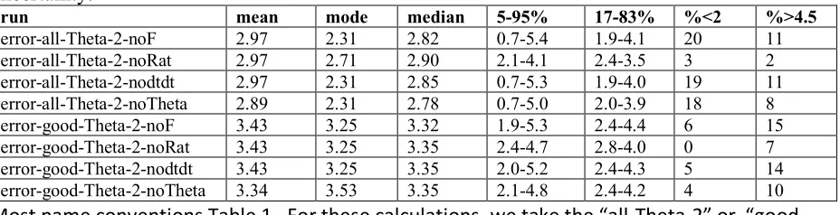
Table 3. Error budget calculations 535
Summary of the statistics of the ECS distribution when one of the input distributions has no 536
uncertainty. 537
run mean mode median 5-95% 17-83% %<2 %>4.5
error-all-Theta-2-noF 2.97 2.31 2.82 0.7-5.4 1.9-4.1 20 11 error-all-Theta-2-noRat 2.97 2.71 2.90 2.1-4.1 2.4-3.5 3 2 error-all-Theta-2-nodtdt 2.97 2.31 2.85 0.7-5.3 1.9-4.0 19 11 error-all-Theta-2-noTheta 2.89 2.31 2.78 0.7-5.0 2.0-3.9 18 8 error-good-Theta-2-noF 3.43 3.25 3.32 1.9-5.3 2.4-4.4 6 15 error-good-Theta-2-noRat 3.43 3.25 3.35 2.4-4.7 2.8-4.0 0 7 error-good-Theta-2-nodtdt 3.43 3.25 3.35 2.0-5.2 2.4-4.3 5 14 error-good-Theta-2-noTheta 3.34 3.53 3.35 2.1-4.8 2.4-4.2 4 10
Most name conventions Table 1. For these calculations, we take the “all-Theta-2” or
“good-538
Theta-2” calculation and sequentially set the uncertainty in one term to zero. The noF”,
“-539
noRat”, “-nodtdt”, and “-noTheta” correspond to no uncertainty in F2xCO2, Qiv/Q4xCO2, ∆TS/∆TA,
540
and Qiv, respectively.
541
543
544 545
Figure 1. (a) Distribution of liv,obs and Qiv,obs (W/m2); (b) scatter plot of R-F (W/m2) vs.
546
TS (K), the dashed line is a least-squares fit; (c) same as panel (b), but the regression is
547
against TA (K).
548 549 550 551 552
[image:23.612.71.540.91.224.2]553
Figure 2. Distribution of liv/l4xCO2 from 25 CMIP5 models; the black dashed line is the
554
mean of the distribution. See methods for description of how the value is calculated in 555
each model. 556
[image:23.612.183.422.354.514.2]558 559 560
[image:24.612.181.430.143.422.2]561
Figure 3. Distributions of ECS using the traditional energy balance framework (Eq. 4). 562
(a) Calculated using liv,obs from the R-F regression, (b) Calculated using liv,obs from the
563
detrended regression. Ò17th %ileÓ and Ò83rd %ileÓ are 17th and 83rd percentile,
564
corresponding to the IPCCÕs likely range. 565
567
Figure 4. Distribution of Qiv/Q4xCO2 from (a) 25 CMIP5 models and (b) from those 15
568
models whose Qiv agrees with observations. The black dashed lines are the means of the
569
distributions. 570
571 572
573
Figure 5. Distribution of ∆TS/∆TA from (a) 25 CMIP5 models and (b) from those 15
574
models whose Qiv agrees with observations. The black dashed lines are the means of the
575
distributions. 576
[image:25.612.129.479.329.475.2]578
Figure 6. Distributions of ECS using the revised energy balance framework (Eq. 6). 579
Panel (a) uses all models for the distributions of Qiv/Q4xCO2 and ∆TS/∆TA, (b) uses all
580
models except for the two GISS models, (c) uses 15 models whose Qiv agrees with the
581
value estimated from observations. All calculations use Qiv,obs from the detrended
582
calculation. Ò17th %ileÓ and Ò83rd %ileÓ are 17th and 83rd percentile, corresponding to
583
the IPCCÕs likely range. 584
586
Figure 7. CMIP5 model estimates of (a) Qiv/Q4xCO2 and (b) Qiv (W/m2). The gray region
587
in panel (b) shows the observational range (from the detrended calculation). The black 588
triangle symbols in panel a) indicate that the modelÕs Qiv agrees with observations; the
589
gray cross symbols indicate that it does not. 590
591 592
593
Figure 8. Error budget analysis of ECS estimates. The ÒallÓ point is the width of the ECS 594
distribution from the good-Theta-2 calculation (Table 3). Then, from left to right, is the 595
width when the uncertainty in forcing, Qiv/Q4xCO2, Qiv,obs, and ∆TS/∆TA distributions are
596
sequentially set to zero. For all points, ÒwidthÓ is the difference between the 17th and 83rd
597
percentile of the ECS distribution. 598
[image:27.612.202.394.461.609.2]Journal of Geophysical Research
Supporting Information for
An estimate of equilibrium climate sensitivity from interannual variability
A.E. Dessler1, P.M. Forster2
1 Dept. of Atmospheric Sciences, Texas A&M University
2 School of Earth and Environment, University of Leeds, UK
Contents of this file
Sect. S1: additional plots of data going into the calculations of liv,obsand Qiv,obs Sect. S2: alternate ways to calculate F2xCO2, liv,obs, and Qiv,obs
Sect. S3: testing models’ ability to estimate ∆TS/∆TA
S1. Data going into the calculations of liv,obs and Qiv,obs
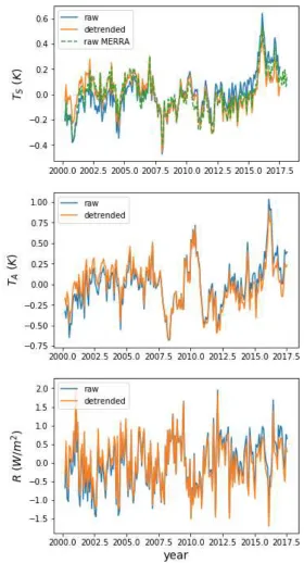
This section shows additional plots of the CERES, temperature, and forcing data. Fig. S1 shows the CERES R time series, the median forcing F time series, and the R-F time series. The CERES data are anomalies (deviations from the mean annual cycle); the forcing data are referenced to pre-industrial. These data go into the R-F estimates of liv,obs and Q iv,obs. Median forcing over
the period analyzed in this paper, relative to preindustrial, is 2.2 W/m2, with 5-95% confidence
interval of 1.1-3.1 W/m2. While the forcing uncertainty is large, what’s important for this
analysis is the uncertainty of the slope of the regression of forcing vs. temperature. Regressing all 10,000 forcing time series vs. TS yields a median value of 0.62 W/m2/K and 5-95% confidence
[image:29.612.134.483.379.581.2]interval of ±0.16 W/m2/K.
Fig. S2 shows the raw and detrended CERES and ERAi temperature data. The detrended time series are used to estimate the detrended liv,obs and Q iv,obs. These two plots show that both
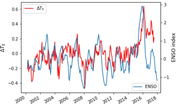
forcing and detrending are minor adjustments to the data. The top panel in Fig. S2 also shows good agreement between ERAi and MERRA2. This supports our analysis that most of the uncertainty in liv,obs and Q iv,obs comes from the scatter in CERES R measurements. Fig. S3 shows the correspondence between ∆TS and the Nino3 index, which demonstrates that most of
the variability in ∆TS is due to interannual variability and not long-term climate change.
Fig. S3. Time series of global average surface temperature anomaly ∆TS (K; left-hand axis) and
Nino3 ENSO index (right-hand axis). ENSO index downloaded from https://www.esrl.noaa.gov/psd/data/timeseries/monthly/NINO3/.
S2. Alternate ways to calculate F2xCO2 and l4xCO2 and Q4xCO2
One potential issue in our calculation is that the forcing we use is from fixed SST runs while the values of l4xCO2 and Q4xCO2 come from abrupt 4xCO2 runs. To evaluate the impact of any
possibly incompatibility, we have also calculated ECS using a distribution of F2xCO2 obtained from
the 4xCO2 runs using the Gregory method [Gregory et al., 2004] (Fig. S4a, Table S1). The ECS
distributions obtained from this (all-Lambda-1-f, good-Lambda-1-f, all-Theta-1-f, good-Theta-1-f) are summarized in Table 1 and 2. ECS estimated using these forcing distributions are close to those using PDRMIP forcing, so we conclude that this is not a significant uncertainty in our analysis.
Another potential issue is that we use of all 150 years of the CMIP5 abrupt 4xCO2 runs to
estimate l4xCO2 and Q4xCO2. It is well known that removal of the first few decades in the Gregory
regression produces a less negative l4xCO2 [e.g., Andrews et al., 2015], which implies a higher
ECS. The effect of this on Q4xCO2 is smaller [Dessler et al., 2018]. To test the impact of this, we
produce ECS estimates where l4xCO2 is calculated from years 20-150 (all-Lambda-1-f_20-150,
good-Lambda-1-f_20-150, all-Theta-1-f_20-150, good-Theta-1-f_20-150). For consistency in these calculations, we use a forcing distribution also derived using these years (Fig. S4b). Note that we call this “quasi-F2xCO2” because it should really not be considered a forcing — it is
Fig. S4. Distribution of F2xCO2 from CMIP5 abrupt 4xCO2 runs. Panel (a) uses all 150 years of the
run, while panel (b) uses years 20-150. The dashed lines are the ensemble averages of 3.45 and 2.94 W/m2.
S3. Testing models’ ability to estimate ∆TS/∆TA
To evaluate the accuracy of the CMIP5 ensemble’s estimate of ∆TS/∆TA, we re-write it as the
product of two terms:
!∀# !∀∃=
!∀#,∋()∗+,− !∀∃
!∀# !∀#,∋()∗+,−
(S1)
where ∆TS and ∆TA are the global average surface temperature and tropical average
atmospheric temperature, respectively, and ∆TS,tropics is the tropical (30°N-30°S) average surface
temperature. The term ∆TS,tropics/∆TA is a measure of the tropical lapse rate, which is
understood to be controlled by moist convective adjustment [Xu and Emanuel, 1989]. Fig. S5a plots monthly average anomalies of ∆TS,tropics vs. ∆TA from the ERAi and, as expected, there is a
clear correlation between these variables. The slope derived from this regression is 0.51±0.06 (5-95% confidence interval).
The ERAi data set, covering 1979-2016 (37 years), contains both long-term warming and
interannual variability. Because of this, we compare the ERAi results to what we consider to be the most analogous model period, the last 37 years of the CMIP5 ensemble’s 150-year abrupt 4xCO2 runs. Ensemble average ∆TS,tropics over this period is 1.07 K, similar to the warming in the
Figure S5. Estimates of ∆TS,tropics/∆TA. (a) Scatter plot of monthly ∆TS,tropics (K; tropical
avg. surface temperature) anomalies vs. ∆TA (K) anomalies from ERAi reanalysis
(1979-2016). The solid line is the best fit line. (b) The slope of the same fit from the last 37 years of the CMIP5 ensemble’s abrupt 4xCO2 runs. The black line and gray region shows
the slope and uncertainty of the fit to observations in panel a.
Figure S6. Estimates of polar amplification in the models, ∆TS/∆TS,tropics. For the CMIP5
ensemble, this is calculated by differencing the average of the first and last decades of the CMIP5 ensemble’s abrupt 4xCO2 runs. The two dashed lines are observational
estimates (see text).
The second term on the right-hand side of Eq. S1, ∆TS/∆TS,tropics, is a measure of polar
amplification in the pattern of surface warming. We estimate this by differencing the averages of the first and last decade of observations or models. The ECMWF 20th century reanalysis [Poli
et al., 2016] produces a value of 1.20 over the years 1900-2010 while the NOAA 20th century
reanalysis project [Compo et al., 2011] produces a value of 1.23 over the years 1851-2014. We estimate this ratio in each CMIP5 abrupt 4xCO2 run and the ensemble agrees well with
[image:33.612.162.450.339.514.2]Such good agreement is not surprising — climate models have long demonstrated considerable skill in simulating the large-scale patterns of surface warming [e.g., Stouffer and Manabe, 2017].
S4. Estimating the distribution of l4xCO2
In the main text, we focus on estimating the distributions of ECS. However, we could also produce an observational estimate of the distribution of l4xCO2. We do this with the following
two equations:
λ/×123 ≈ λ56,789:;×<=> :+?
(S2)
λ/×123 ≈ Θ56,789 Α;×<=>
Α+? !∀∃ !∀#
(S3)
We use the same Monte Carlo approach we did in the main text: distributions of Qiv,obs and liv,obs come from the observations and distributions of liv/l4xCO2, Qiv/Q4xCO2, and ∆TS/∆TA come
from the CMIP5 models. The resulting distributions are summarized in Tables S2 and S3. We note that the Q calculations provide a consistent bound for l of -0.7 to -1.5 W/m2/K (17-83%
Table S1. Values for individual models
Model liv Qiv l4xCO2 Q4xCO2 ∆TS/∆TA F2xCO2
ACCESS1-0 -0.69 -1.22 -0.75 -0.77 0.96 2.88
ACCESS1-3 -0.66 -0.86 -0.82 -0.74 0.91 2.91
BCC-CSM1-1 -0.74 -0.89 -1.21 -1.12 0.93 3.38
BCC-CSM1-1-M -0.91 -0.94 -1.31 -1.23 0.92 3.69
CCSM4 -1.26 -1.25 -1.24 -1.26 0.99 3.63
CNRM-CM5 -1.14 -1.25 -1.11 -1.01 0.94 3.63
CNRM-CM5-2 -1.01 -1.25 -1.06 -0.94 0.89 3.64
CanESM2 -0.77 -0.73 -1.03 -0.90 0.88 3.80
FGOALS-g2 -1.55 -1.25 -0.83 -0.85 1.00 2.82
FGOALS-s2 -1.35 -1.60 -0.88 -0.77 0.87 3.75
GFDL-CM3 -0.21 -0.63 -0.75 -0.63 0.80 2.94
GFDL-ESM2G -0.80 -1.24 -1.42 -0.98 0.68 3.33
GFDL-ESM2M -1.41 -1.12 -1.34 -0.92 0.74 3.26
GISS-E2-H -1.48 -0.36 -1.57 -1.36 0.91 3.70
GISS-E2-R -1.03 -0.16 -1.70 -1.35 0.77 3.64
INMCM4 -0.65 -0.83 -1.51 -1.18 0.80 3.07
IPSL-CM5A-LR -0.57 -0.61 -0.79 -0.54 0.71 3.19
IPSL-CM5A-MR -0.46 -0.33 -0.81 -0.54 0.68 3.32
IPSL-CM5B-LR -0.93 -0.94 -1.00 -0.87 0.91 2.61
MIROC5 -1.18 -0.90 -1.58 -1.13 0.84 4.25
MPI-ESM-LR -0.78 -0.72 -1.14 -0.91 0.81 4.11
MPI-ESM-MR -0.69 -0.76 -1.18 -0.93 0.80 4.08
MPI-ESM-P -0.72 -0.70 -1.25 -0.98 0.80 4.32
MRI-CGCM3 -0.58 -1.29 -1.26 -1.11 0.88 3.27
NorESM1-M -1.19 -1.13 -1.11 -1.15 1.02 3.10
Units on l and Q are W/m2/K, ∆T
S/∆TA is unitless; F2xCO2 is derived from that modelÕs abrupt
Table S2. l4xCO2 estimated from Eq. S2
run mean mode median 5-95% 17-83%
all-Lambda-1 -0.73 -0.63 -0.64 -1.9 to +0.2 -1.3 to -0.2
all-Lambda-2 -1.16 -0.95 -1.03 -2.6 to -0.2 -1.8 to -0.5
good-Lambda-1 -0.85 -0.79 -0.78 -2.1 to +0.2 -1.5 to -0.2
good-Lambda-2 -1.20 -0.95 -1.07 -2.6 to -0.2 -1.8 to -0.5
See Table 1 for a description of the runs. Units are W/m2/K.
Table S3. l4xCO2 estimated from Eq. S3
run mean mode median 5-95% 17-83%
all-Theta-1 -1.41 -1.11 -1.00 -4.2 to -0.5 -1.5 to -0.7
all-Theta-2 -1.56 -1.11 -1.11 -4.6 to -0.6 -1.6 to -0.8
all-Theta-1-corr -1.41 -1.11 -1.00 -4.2 to -0.5 -1.5 to -0.7
good-Theta-1 -1.01 -1.11 -0.96 -1.6 to -0.6 -1.3 to -0.7
good-Theta-2 -1.05 -1.11 -0.99 -1.6 to -0.6 -1.4 to -0.8
good-Theta-1-corr -1.01 -1.11 -0.96 -1.6 to -0.6 -1.3 to -0.7
noGISS-Theta-1 -1.00 -1.11 -0.96 -1.6 to -0.5 -1.4 to -0.7
noGISS-Theta-2 -1.11 -1.11 -1.07 -1.8 to -0.6 -1.5 to -0.8
[image:36.612.74.535.204.351.2]