processing
.
White Rose Research Online URL for this paper:
http://eprints.whiterose.ac.uk/124737/
Version: Accepted Version
Article:
Anbiyaei, M., Liu, W. orcid.org/0000-0003-2968-2888 and McLernon, D. (2017) White
noise reduction for wideband linear array signal processing. IET Signal Processing. ISSN
1751-9675
https://doi.org/10.1049/iet-spr.2016.0730
This paper is a postprint of a paper submitted to and accepted for publication in IET Signal
Processing and is subject to Institution of Engineering and Technology Copyright. The
copy of record is available at the IET Digital Library
[email protected] https://eprints.whiterose.ac.uk/
Reuse
Unless indicated otherwise, fulltext items are protected by copyright with all rights reserved. The copyright exception in section 29 of the Copyright, Designs and Patents Act 1988 allows the making of a single copy solely for the purpose of non-commercial research or private study within the limits of fair dealing. The publisher or other rights-holder may allow further reproduction and re-use of this version - refer to the White Rose Research Online record for this item. Where records identify the publisher as the copyright holder, users can verify any specific terms of use on the publisher’s website.
Takedown
If you consider content in White Rose Research Online to be in breach of UK law, please notify us by
White Noise Reduction for Wideband Linear Array
Signal Processing
Mohammad Reza Anbiyaei
†, Wei Liu
†and Des C. McLernon
∗†
Communications Research Group, Department of Electronic and Electrical Engineering, University of Sheffield,
Sheffield S1 3JD, U.K.
∗
Signal Processing for Communications Group, School of Electronic and Electrical Engineering,
University of Leeds, Leeds LS2 9JT, U.K.
Abstract
The performance of wideband array signal processing algorithms is dependent on the noise level in the system. A method is
proposed for reducing the level of white noise in wideband linear arrays via a judiciously designed spatial transformation followed
by a bank of highpass filters. A detailed analysis of the method and its effect on the spectrum of the signal and noise is presented.
The reduced noise level leads to a higher signal to noise ratio (SNR) for the system, which can have a significant beneficial
effect on the performance of various beamforming methods and other array signal processing applications such as direction of
arrival (DOA) estimation. Here we focus on the beamforming problem and study the improved performance of two well-known
beamformers, namely the reference signal based (RSB) and the linearly constrained minimum variance (LCMV) beamformers.
Both theoretical analysis and simulation results are provided.
Index Terms
White noise reduction, uniform linear arrays, nonuniform linear arrays, wideband beamforming, direction of arrival estimation,
performance analysis.
I. INTRODUCTION
Wideband array signal processing, including beamforming and direction of arrival (DOA) estimation, has various applications
in radar, sonar and wireless communications, and has been studied extensively in the past [1]–[9]. The performance of wideband
array signal processing algorithms is dependent on the level of noise in the system, and normally the lower the level of noise,
the better is the performance. Many methods have been developed in the past to reduce the noise level of a system, and one
example is adaptive noise cancellation (ANC), which uses a reference undesired noise source and a primary source contaminated
by noise, followed by adaptive filtering to produce a cleaned result [10], [11].
One common assumption for noise in wideband arrays is that it is both spatially (and in many cases also temporally) white.
That is, the noise at one array sensor is uncorrelated with that at other sensors. Under this assumption, it seems that there is not
much we can do about it and we have to simply accept whatever is left of the noise component after processing the signals.
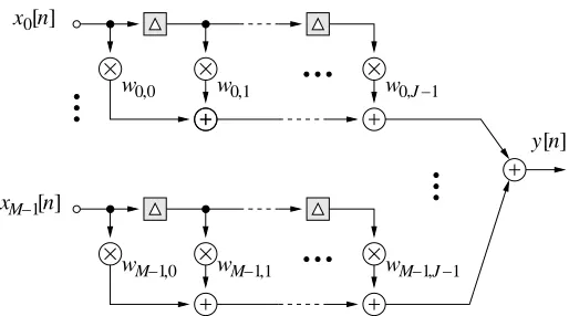
For example, in the simplest beamforming structure shown in Fig. 1a, the beamformer output y[n] is a linear combination
array sensors
]
[n
1
x
]
[n
x
0M−1
[n
]
x
]
[
y
w
n
w
01
w
M−1
(a) A simple beamformer with its outputy[n]given by
a linear combination of the received array signalsx0[n],
x1[n],···,xM−1[n]weighted with the coefficientsw0,w1,
···, wM−1.
, , ,0
,0 ,1
,1
n
M−1 M−1
M−1
w0 w0 −1J
M−1[n] x
] [ x0
w w w J−1
] [ y n w0
[image:3.612.178.435.263.406.2](b) A general wideband beamformer withMsensors andJtaps.
Figure 1: General structure of narrowband and wideband beamformers
The question here is, whether there is anything that we can do to reduce the effect of white noise in a wideband array system
(without attenuating the directional signals) so that the performance of the subsequent processing (such as DOA estimation
and beamforming) could be improved.
In this paper, we aim to answer that question by developing a novel method to reduce the white noise level of a wideband
array using a combination of a set of judiciously designed spatial transformations and a bank of filters, and the key is to
realize that the white noise and the directional wideband signals received by the array have different spatial characteristics.
Based on this difference, and motivated by the low-complexity subband-selective adaptive beamformer proposed in [12], we
first transform the received wideband sensor signals into a new domain where the directional signals are decomposed in such
a way that their corresponding outputs are associated with a series of tighter and tighter highpass spectra, while the spectrum
of noise still covers the full band from −π toπ in the normalized frequency domain. Then, a series of highpass filters with
different cutoff frequencies are applied to selectively remove part of the noise spectrum while keeping the directional signals
unchanged. Finally, an inverse transformation is applied to the filtered outputs to recover the original sensor signals, where
compared to the original set of received sensor signals, the directional signals are left intact while the noise power has been
reduced. The main assumption of the work is that the spectrum of the noise is white, and the noise between the sensors is
1
θ
−1
n
[ ]
n
[ ] [ ]n
n
[ ]
n
[ ]
n
[ ]
n
[ ]
n
[ ]
n
[ ]
n
[ ]
n
[ ]
n
[ ]
n
[ ] [ ]n [ ]n
−1
M M−1 M−1 M−1
−1 M
^ ^
x x
x
q q
z z
x x h
h
h
A
A
0
1 0
1
0
1
q z x^
1
[image:4.612.185.430.54.158.2]0 0
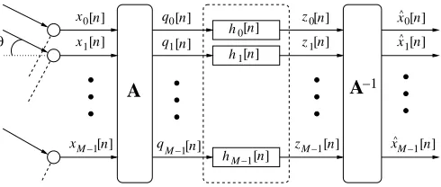
Figure 2: A block diagram for the general structure of the proposed noise reduction approach.
noise is correlated between the sensors, a different analysis would be needed.
Compared to our earlier published work in [13], where the idea was applied to uniform linear arrays (ULAs) for DOA
estimation, in this paper, we extend it to arbitrary linear arrays and also focus on the beamforming problem. In particular, we
give a detailed analysis of the spectrum of noise at different stages of the processing and provide theoretical results to show
the improved performance; in addition, to accommodate the nonuniform linear array (NLA) geometry, a new design for the
transformation matrix is proposed.
One condition placed on the transformation matrix is that it must be invertible. We have further assumed that it is also
unitary and thus the discrete Fourier transform (DFT) matrix is used as a representative example for the ULA case and a
least squares based design is introduced for the NLA case. Detailed analysis shows that the signal to noise ratio (SNR) of the
array after the proposed processing can be improved by about 3dB in the ideal case. This is then translated into improved
performance for beamforming, as demonstrated by both theoretical analysis and simulation results. Here we focus on two
well-known beamformers, namely the reference signal based (RSB) [14]–[17], and the linearly constrained minimum variance
(LCMV) beamformers [2], [18], [19].
This paper is organized as follows. In Section II, the general structure of our proposed method is first introduced. In
Section III, the DFT matrix as a choice for the transformation matrix for ULAs is studied and the spectrum of noise at
different stages of the processing is analysed. In Section IV, the adaptive beamformers and the effect of the noise reduction
method on their correlation values are explained in detail. Extension of the method to the NLA case is provided In Section V.
Simulation results based on the two adaptive beamformers are presented in Section VI in comparison with the theoretical
results, and conclusions are drawn in Section VII.
II. GENERALSTRUCTURE OF THE PROPOSED METHOD
Consider an M-element arbitrary linear array. A block diagram for the general structure of the proposed method is shown
in Fig. 2. The M received array signals xm[n], m=0, . . . ,M−1, are first processed by an M×M transformation matrix A,
and then its outputs qm[n], m=0, . . . ,M−1, pass through a bank of highpass filters with impulse responses given by hm[n],
m=0, . . . ,M−1. The outputs of these filters are denoted by zm[n],m=0, . . . ,M−1 and these are then transformed by the
M×M inverse transformation A−1. For simplicity we assume A is unitary, i.e., A−1=AH, where {·}H denotes Hermitian transpose.
There are two components for the received array signal xm[n] at them-th sensor: the signal part sm[n] and the white noise
part bm[n]. So we have:
The total signal vector x[n]can be expressed as
x[n] =s[n] +b[n], (2)
where
x[n] = [x0[n],x1[n],···,xM−1[n]]T,
s[n] = [s0[n],s1[n],···,sM−1[n]]T,
b[n] = [b0[n],b1[n],···,bM−1[n]]T.
Applying the M×M transformation matrixAto the signal vector x[n], we obtain the output signal vectorq[n] as
q[n] =Ax[n], (3)
where
q[n] = [q0[n],q1[n],···,qM−1[n]]T.
The element of Aat the m-th row andl-th column is denoted by am,l, i.e.,[A]m,l=am,l. Each row vector of A acts as a
simple beamformer, and its output qm[n] is given by
qm[n] = M−1
∑
l=0
am,lxl[n]. (4)
The beam response Rm(Ω,θ)of this simple beamformer as a function of the normalized frequencyΩ and the DOA angle θ
is [12], [20],
Rm(Ω,θ) = M−1
∑
l=0
am,le−iµlΩsinθ, (5)
whereµl=dl/cTsandΩ=ωTs, withdl being the distance from the zero-th sensor to thel-th sensor (whered0=0),cthe wave
propagation speed, Ts the sampling period, and ω the angular frequency of signals.
With ˆΩ=Ωsinθ, we can obtain an alternative representation ofRm(Ω,θ)as follows
Am(Ωˆ) = M−1
∑
l=0
am,le−iµl ˆ
Ω,
(6)
where ˆΩ is representing the spatial frequency of the received signal,Am(Ωˆ)is the frequency response of them-th row vector
of the M×M transformation matrixA(if we consider each row vector as the impulse response of a finite impulse response
(FIR) filter).
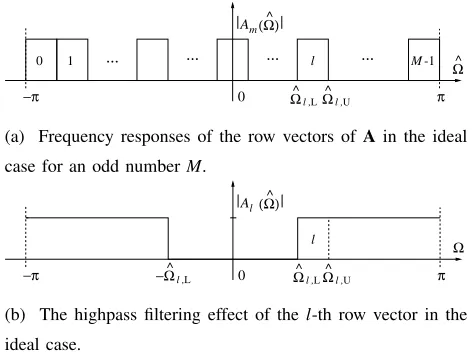
Similar to [12], the frequency responses Am(Ωˆ),m=0,1,···,M−1, are arranged to be bandpass, each with a bandwidth
2π/M. The row vectors of A all together cover the whole frequency band which is [−π:π]. An ideal example for an odd
numberM is shown in Fig. 3a.
The bandpass filters, which are used as row vectors of A, have a highpass filtering effect on the received array signals. To
examine this highpass behaviour, the l-th row vector is analyzed. The frequency response of this row vector is shown in Fig.
3a, which is:
Al(Ωˆ)
=
1, for ˆΩ∈[Ωˆl,L: ˆΩl,U]
0, otherwise.
(7)
As sinθ ∈[−1 : 1] when θ ∈[−π/2 :π/2], the possible maximum frequency component of the l-th row vector Al(Ωˆ) is
Ω=π, which corresponds to|sinθ|=Ωˆl,U/π when ˆΩl,L≥0, while the minimum frequency component is Ω=Ωˆl,L, which
Ω^l ,LΩ^
M -1 ^
(Ω)
... ... ... ...
l ,U
−π π
l
0
^
Ω
0 1
m A
(a) Frequency responses of the row vectors ofAin the ideal
case for an odd numberM.
Ω^l ,LΩ^l ,U
^
(Ω)
−π π
l
0
l ,L
^
−Ω
Ω l
A
(b) The highpass filtering effect of thel-th row vector in the
[image:6.612.188.424.55.235.2]ideal case.
Figure 3: Frequency responses of the row vectors of A in the ideal case and the highpass filtering effect of a sample row
vector.
|Al(Ωsinθ)|=
1, for Ω∈[Ωˆl,L:π]
0, otherwise.
(8)
as shown in Fig. 3b.
Considering the above frequency response, the received array signal components with frequency ofΩ∈[−Ωˆl,L: ˆΩl,L]will
not “pass” through this row vector, since ˆΩ=Ωsinθ does not fall into the passband of[Ωˆl,L: ˆΩl,U], no matter what value the
DOA angle θ takes. Therefore, the frequency range of the output is |Ω| ≥Ωˆl,L and the lower bound is determined by ˆΩl,L
when ˆΩl,L>0. Alternatively, the lower bound is determined by |Ωˆl,U| when ˆΩl,L<Ωˆl,U<0.
As a result, the output spectrum of the directional signal part of ql[n] corresponding to the l-th row vector will then be
highpass filtered as shown in Fig. 3b. As the noise part in x[n]is spatially white, the output noise spectrum of the row vector
is still a constant, covering the whole spectrum. As shown in Fig. 2, the output ql[n] of each row vector is the input to a
corresponding highpass filterhl[n],l=0,1,···,M−1. These highpass filters should cover the whole bandwidth of the signal
part of the outputql[n]and therefore have the same frequency response as specified in Fig. 3b. As a result, in the ideal case,
the highpass filters will not have any effect on the signal components and all the signal components will pass through the
highpass filters without any distortion. But then the frequency components of the white noise falling into the stopband of these
highpass filters will be removed.
The output of the highpass filters is the convolution of each row vector output and its corresponding highpass filter,
z[n] =
z0[n] .. .
zM−1[n]
=
q0[n]∗h0[n] .. .
qM−1[n]∗hM−1[n]
, (9)
where∗ denotes the convolution operator.
Now we consider the noise reduction effect of these filters. Each filter removes part of the noise except for that part
corresponding to the row vector with a frequency response covering the zero frequency component, which should allow all
frequencies to pass. Assume now that the size M of the array is an odd number. From Fig. 3, for the first row vectorA0(Ωˆ),
response covering the zero frequency, all of the noise will pass. For the row vectors with frequency responses larger than
the zero frequency, the highpass filtering is a replica of the bands with frequency responses lower than the zero frequency.
Therefore, in the ideal case, the ratio between the total noise power after and before the processing of the M highpass filters
can be expressed as
Pbo
Pbi
= 1
M
1+2
2
M+
4
M+···+ M−1
M
, (10)
wherePbois the total noise power at the output of the filters andPbiis the total noise power at their input. Following the same
procedure, if the size of the array is an even number, then this ratio is given by
Pbo
Pbi
= 1
M
1+2
3
M+
5
M+···+ M−1
M
+ 1
M
. (11)
As a result, we have
r(M) =Pbo
Pbi =
M2+2M−1
2M2 , if M>1 is odd
M2+2M−2
2M2 , if M>2 is even.
(12)
WhenM→∞, noise power will be reduced by half in both cases. Since the highpass filters have no effect on the signal part,
the ratio between the total signal power and the total noise power will be improved by almost 3dB in the ideal case. For a
finiteM, the improvement will be less than 3dB. For example, whenM=16, it is about 2.53dB.
Applying the inverse of the transformation matrix A−1=AH (with size M×M) to z[n], we obtain the estimates of the original input sensor signals ˆxm[n],m=0,1,···,M−1. In vector form, we have
ˆ
x[n] =A−1z[n], (13)
where ˆx[n] = [xˆ0[n],xˆ1[n],···,xˆM−1[n]]T.
After going through these processing stages, there is no change in the signal part at the final output ˆxl[n],l=0,1,···,M−1
compared to the original signal part in xl[n], l=0,1,···,M−1. On the contrary, since A−1 is also unitary, the total noise power stays the same between ˆx[n] andz[n], which is almost half the total noise power inx[n]. Therefore, for a very large
array size M, we have
kxˆ[n]k2
2≈ ks[n]k22+ 1 2kb[n]k
2
2. (14)
wherek.k2 is thel2norm.
Based on above discussion, in terms of the total signal power to total noise power ratio (TSNR), we have the following
relationship
T SNRxˆ≈ k s[n]k2
2 1 2kb[n]k22
=2T SNRx. (15)
So in the ideal case, for a very largeM, the TSNR is almost doubled by the proposed noise reduction method. This can be
translated into better performance for different array processing applications such as beamformering and DOA estimation. In
the following section, using the DFT-based transformation matrix for ULAs, we analyse the theoretical result for two commonly
used beamformers to show the performance improvement in the ideal case.
III. ANALYSISBASED ON THEDFT MATRIX FORULAS
The transformation matrix is the most important part of the system. It should have a full rank so that an inverse transform
can be applied at the end to recover the signals. Another key requirement is to make sure its row vectors have the desired
a constrained FIR filter design problem. This is similar to the beamspace transformation problem studied in [21]–[23], and
as pointed out there, we could design a prototype lowpass filter and then modulate it to different frequency bands by a DFT
operation or use the DFT matrix directly. In particular, the DFT matrix is unitary, which will simplify our theoretical analysis
and provide us with the crucial insight into the performance of the proposed structure.
Using the DFT matrix for an M×M transformationA, withγ=e−i(2π/M), we have
A=√1
M
γ0·0 γ0·1 . . . γ0·(M−1) γ1·0 γ1·1 . . . γ1·(M−1)
..
. ... . .. ...
γ(M−1)·0 γ(M−1)·1 . . . γ(M−1)·(M−1) . (16)
Next, an analysis of the signal spectrum based on such a transformation matrix at different stages of the proposed structure
is provided.
A. Spectrum Analysis with DFT Matrix
Now we study the input-output relationships in the frequency domain based on the DFT matrix. We first have
ˆ
x(Ω) =A−1HAx(Ω), (17)
where ˆx(Ω)andx(Ω)are the vectors holding the discrete-time Fourier transforms (DTFTs) of the time-domain signal vectors
ˆ
x[n] and x[n], respectively, and H is an M×M real valued diagonal matrix with its diagonal elements being the frequency
responses Hm(Ω)of the corresponding filtershm[n],m=0,1,···,M−1, i.e.,
H=
H0(Ω) 0 . . . 0
0 H1(Ω) . . . 0
..
. ... . .. ...
0 0 . . . HM−1(Ω)
. (18)
From (17), the transfer function of the system is:
T=A−1HA=
A−1√1
M
H0γ0·0 ··· H0γ0·(M−1)
H1γ1·0 ··· H1γ0·(M−1) ..
. . .. ...
HM−1γ(M−1)·0) ··· HM−1γ(M−1)·(M−1) . (19)
Then, all the elements of T (complex valued, with size M×M) can be obtained. Considering the relationship between the
terms, we can derive a general form for the elements of Tand the element at theu-th row andv-th column is given by
Tu,v= 1
M
M−1
∑
l=0
Hlγ−luγlv= 1
M
M−1
∑
l=0
Hlγl(v−u). (20)
So we have
ˆ
x(Ω) =Tx(Ω). (21)
We are interested in the spectrum of the noise at the output. The relationship between the input and output signals’ spectrum
is [24],
−10 −0.5 0 0.5 1 0.2
0.4 0.6 0.8 1
Power Spectral density /
σ
2 n
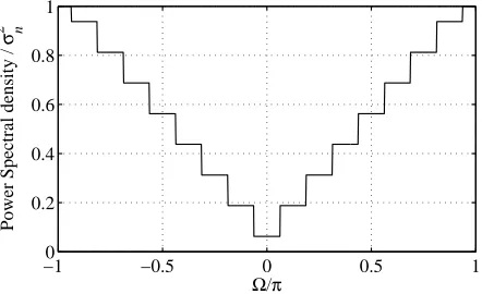
[image:9.612.188.409.64.199.2]Ω/π
Figure 4: Power spectrum of the output of the noise reduction system withM=16.
Sxˆ(Ω)andSx(Ω)areM×Mmatrices, where each matrix element represents the cross-spectral density of the two corresponding
signals.Sx(u,v)is the(u,v)-th element ofSxand it is the cross-spectral density betweenxu[n]andxv[n]. It can be easily proved
that the cross spectral density is equal to the DTFT of the cross correlation function of the two signals [25]. Then we have
Sx(u,v) =xu∗(Ω)xv(Ω), (23)
where the asterisk denotes the complex conjugate. Similarly, we have Sxˆ(u,v) =xˆ∗u(Ω)xˆv(Ω). Now we consider the noise part. The spectral density of the white noise is σ2
b, whereσb2 is the variance of the noise. Since
the noise received by each array sensor is uncorrelated, the noise spectral density of a sensor is Sb(u,u) =σb2 and the noise
cross spectral density between two sensors isSb(u,v) =0. So, the spectrum of the noise received by the array is:
Sb(Ω) =σb2
1 0 ··· 0
0 1 ··· 0
..
. ... . .. ...
0 0 ··· 1
=σb2I, (24)
whereIis the M×M identity matrix. Therefore, (22) can be written as
Sbˆ(Ω) =TT∗(Ω)σ 2
bI. (25)
Sbˆ(Ω)is anM×M complex valued matrix with real values on the diagonal. Each term ofSbˆ(Ω)is given by:
Sbˆ(u,v)(Ω) = σ2
b
M
M−1
∑
l=0
Tu,lTv∗,l. (26)
From (20) and (26), we have:
Sbˆ(u,v)(Ω) = σ2
b
M
M−1
∑
l=0
Hl(Ω)ei2Mπ(u−v)l. (27)
The spectrum of the noise forM=16 is shown in Fig. 4 in the ideal case. The next step is to take the inverse DTFT from
(27) to calculate the correlation function in the time domain. The inverse Fourier transform of (27) is:
Rbˆ(u,v)(τ) = DTFT−1 (
σ2 b
M
M−1
∑
l=0
Hl(Ω)ei2Mπ(u−v)l )
= σ
2 b
M
M−1
∑
l=0
whereτ is an arbitrary delay andRbˆ(u,v)(τ)is the correlation function between the filtered noise at theu-th and the v-th array
elements after applying the noise reduction method. As the only term which is a function of frequency is Hl(Ω), the inverse
DTFT only applies to this part. The frequency response of a single highpass filter has the same form as that shown in Fig. 3b.
To calculate DTFT−1{Hl(Ω)}, (28) can be written as
Rbˆ(u,v)(τ) = σ2
b
M
M−1
∑
l=0
π−Ωˆl,L
π e
i2Mπ(u−v)leiπ+
ˆ
Ωl,L
2 τsinc(π−
ˆ Ωl,L
2 τ), (29)
where π is the maximum normalized frequency and ˆΩl,L is the lower bound frequency of the l-th highpass filter as was
previously shown in Fig. 3b. The correlation values regarding different time delays can be calculated from (28) and will be
used when we derive the theoretical performance results for different wideband beamformers.
IV. PERFORMANCE ANALYSIS OF THE PROPOSED METHOD FORADAPTIVEWIDEBANDBEAMFORMING
For wideband beamforming, a tapped delay-line (TDL) is normally employed, with Fig. 1b showing a general structure.
The TDL has a length of J and the coefficient for them-th sensor at the j-th position of the TDL is denoted by wm,j. All J
weights at the m−th TDL form anelement weight vector wm and allM element weight vectors form aMJ×1 total weight
vector w, where
wm= [wm,0,wm,1,···,wm,J−1]T, (30)
w=
wT0,wT1,···wTM−1T. (31)
The beamformer output y[n]is given by
y[n] =wTx, (32)
where the input signal vector x is defined as
x =
xT[n] xT[n−1] . . . xT[n−J+1]T (33)
x[n−j] = [x0[n−j] x1[n−j] . . . xM−1[n−j]]T . (34)
The idea is to process the received array signal by the noise reduction method, so that the noise level in received signal
will be reduced; then, the recovered array signals with reduced noise level will be fed to the following beamformers. In the
following, two widely-used adaptive beamforming methods are briefly reviewed and the theoretical performance results are
then derived based on the proposed noise reduction method.
A. Reference Signal Based Adaptive Beamformer
The reference signal based (RSB) beamformer is normally employed when a reference signal r[n] is available, where the
weight vector of the beamformer can be adjusted to minimize the mean square error (MSE) between the reference signal and
the beamformer output y[n][14], [15], [17], [26]. TheMJ×1 optimal weight vector is given by:
wopt=ΦΦΦx−1sd, (35)
whereΦΦΦx is the signal correlation matrix with sizeMJ×MJ,
Φ Φ
Φx=E[x∗xT], (36)
(E{·}denotes the statistical expectation) andsd is the reference correlation vector with sizeMJ×1,
withr0[n]being the normalized reference signal with unit power.
There are three components for each of the received sensor signals: desired signal, interference and noise. So, the signal
vector xcan be decomposed into three corresponding parts:
x=xd+xi+xb. (38)
Since the desired signal, interference and noise are uncorrelated with each other,ΦΦΦx can be decomposed into threeMJ×MJ
correlation matrices corresponding to the desired signal, interference and white noise components, respectively. i.e.,
ΦΦΦx=ΦΦΦd+ΦΦΦi+ΦΦΦb. (39)
Assuming the reference signal is the same as the desired signal,sd in (37) can be simplified to
sd=E[x∗ro[n]] =E[x∗dro[n]]. (40)
More details for calculating wopt from (35) can be found in [15].
For our proposed noise reduction method, in the ideal case the directional signals (desired and interference) remain intact
and only the noise part is reduced/changed. Then, the total signal vector ˆx corresponding to x after noise reduction can be
expressed as:
ˆ
x=xd+xi+xˆb. (41)
where ˆxbis the part of ˆx corresponding to the reduced noise after the proposed processing.
Similarly the correlation matrices ΦΦΦd andΦΦΦi will remain the same after noise reduction, but the correlation matrix for the
noise part will be changed toΦΦΦˆ
b with size MJ×MJ. Then, the MJ×MJ correlation matrixΦΦΦxˆ after noise reduction can be
expressed as:
ΦΦΦxˆ=ΦΦΦd+ΦΦΦi+ΦΦΦˆ
b. (42)
We can obtainΦΦΦˆ
b from (28) and partition it intoM×M submatrices (each submatrix isJ×J),
Φ Φ Φˆ
b=
Φ ΦΦˆ
b0,0 ··· ΦΦΦbˆ0,M−1
..
. . .. ...
Φ Φ Φˆ
bM−1,0 ··· ΦΦΦbˆM−1,M−1
. (43)
whereΦΦΦˆ
bu,v=E[ˆx ∗
ˆ buxˆ
T ˆ
bv]. The delay between two adjacent taps in a TDL isT0=
πr
2Ω0, where Ω0 is the centre frequency andr is the number of quarter-wave delays in T0at frequencyΩ0. Hence the delay between the j-th andk-th tap isτ= (j−k)T0.
Therefore the correlation value[ΦΦΦbu,v]j,k between the noise (after the proposed processing) at the j-th tap of theu-th element
and that at thek-th tap of the v-th element is given by
[ΦΦΦbu,v]j,k=E[b∗u,j[n]bv,k[n] =Rb(u,v)[(j−k)T0]. (44)
With the result in (29), we have
[ΦΦΦbu,v]j,k= σ2
b
M
M−1
∑
l=0
π−Ωˆl,L
π e
i2Mπ(u−v)leiπ+
ˆ
Ωl,L
2 (j−k)T0×sinc(π−Ωˆl,L
2 (j−k)T0). (45)
Now we have all the correlation values required for calculating the wopt in (35) and the beamformer outputy[n]is
with its power given by
P=1
2E[ky[n]k 2] =1
2w H
optΦΦΦxˆwopt;. (47)
The output SINR is given by
SINR= Pd
Pi+Pbˆ
(48)
where
Pd = wHoptΦΦΦdwopt (49)
Pi = wHoptΦΦΦiwopt (50)
Pbˆ = w H
optΦΦΦbˆwopt. (51)
B. Linearly Constrained Minimum Variance Beamformer
In practice, the reference signal assumed in Section IV-A may be unavailable. However, when some information on the
DOAs as well as the bandwidth limits of the desired signal and/or the interferences is available, a linearly constrained minimum
variance (LCMV) beamformer can be employed for effective beamforming [2], [27]. The LCMV beamformer is formulated
as follows (based on the recovered signal ˆx after the proposed noise reduction method),
min
w w
HΦΦΦ ˆ
xw subject to CHw=f, (52)
wherewandΦΦΦxˆ are defined as before in Section IV-A, Cis theMJ×J constraint matrix andf is theJ×1 response vector.
The solution to (52) can be obtained using the Lagrange multipliers method,
wopt=ΦΦΦ−xˆ1C(CHΦΦΦ−xˆ1C)−1f. (53)
Suppose the desired signal comes from the broadside, i.e., θd=0◦. Then, Candf have a very simple form [2]. With the optimal weight vector determined, the output SINR can be obtained as in Section IV-A.
V. EXTENSION OF THE NOISE REDUCTION METHOD FORNLAS
As an example for a unitary matrix with a good bandpass response, we have considered the DFT matrix in the ULA case.
However, the DFT matrix is not applicable for the NLA case, since it does not have a uniform spacing, and the resultant beams
by each row vector of such a transformation will be significantly distorted.
Therefore, we use a different approach for designing the transformation matrix for NLAs by introducing a least squares
based design method here. The idea is to use an ideal unitary beam response such as those of a DFT matrix as the reference
response for the least squares method to design a prototype filter p(where [p]l=pl,l=0,···,M−1), and then we modulate
it into different subbands in a uniform way to form the required transformation matrix.
The least squares filter design method has been well studied in the past [2], [28]. Given the desired beam patternPd(Ωˆ)and
consideringd(Ωˆ)as the steering vector of the NLA,
d(Ωˆ) =
1 e−i d1
cTsΩˆ ··· e−idMcTs−1Ωˆ
, (54)
the problem can be solved by minimizing the sum of squares of the error between Pd(Ωˆ) and the designed response P(Ωˆ)
over the frequency range of interest, i.e.,
min
p
∑
ˆ
Ωpb
Minimizing the above cost function with respect to the coefficients vectorp gives the standard least squares solution,
popt=G−ls1gls, (56)
with
Gls=
∑
ˆΩpb
d(Ωˆ)dH(Ωˆ),
gls=
∑
ˆ
Ωpb
(dR(Ωˆ)Pd,R(Ωˆ) +dI(Ωˆ)Pd,I(Ωˆ)),
wheredR(Ωˆ)andPd,R(Ωˆ)denote the real parts of d(Ωˆ)andPd(Ωˆ), anddI(Ωˆ)andPd,I(Ωˆ)are their imaginary parts.
Then, we modulate pto cover the whole normalized frequency band,
Am,l=e−i2MπmcTsdl pl, (57)
wherem=0,···,M−1, l=0,···,M−1.
At this stage if the condition number of the resultant transformation matrix is high, we can use the diagonal loading
method [29] to reduce the condition number,
AL=A+αI, (58)
whereα is a constant representing a small loading level.
Note that the transformation matrix obtained by the above procedure will not be unitary in general and how to design a
unitary matrix for NLAs with the required bandpass filtering effect is still an open problem for our future research. However,
we will see in the simulations part that the transformation matrix obtained from the above procedure works well to some
degree and provides a clear performance improvement.
VI. SIMULATIONRESULTS
In this section, simulation results will be provided for both ULAs and NLAs, and the performance improvement by the
proposed noise reduction (NR) method for RSB and LCMV beamformers will be examined.
A. Performance of the NR Method for ULA
The simulations here are based on a 16-sensor (M=16) ULA and the desired signal arrives from the broadside (θd=0).
The received signals are processed by the 16×16 DFT-based transformation matrix and pass through the highpass filters. We
have assumed that the highpass filters have an ideal brick-wall shape response and to have a close approximation, linear-phase
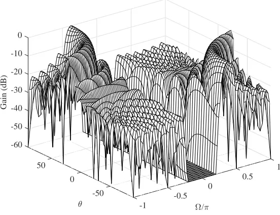
101-tap FIR filters with a common delay of 50 samples are employed. The beam pattern of a sample row vector with respect
to signal frequency Ω and DOA angleθ before and after highpass filtering is shown in Fig. 5.
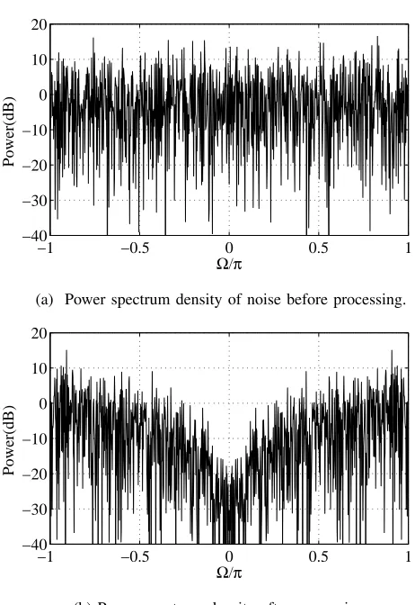
1) Effect on noise and directional signals: To see the effect of the whole system on noise, we generate spatially and
temporally white noise at the array sensors with unit power. The power spectrum density of noise before and after the
proposed noise reduction process is shown in Fig. 6a and Fig. 6b, respectively. It can be seen that the noise power has been
reduced significantly at lower frequencies, while for higher frequencies, the reduction becomes less and less. Overall the power
of noise has been reduced clearly.
For the received directional signals, as discussed there should not be any change after the proposed processing in the ideal
-1 -0.5 0 0.5 1 /
-50 -40 -30 -20 -10 0
Gain (dB)
(a) 2D beampattern of a sample row vector.
-60 -50 -40
50 1
-30
Gain (dB)
-20
0.5 0
-10
/ 0
0
-50 -0.5
-1
(b) 3D beampattern of the row vector shown in Fig. 5a before highpass filtering.
-60 -50 -40
50 1
-30
Gain (dB)
-20
0.5 0
-10
/ 0
0
-50 -0.5
-1
[image:14.612.164.440.506.718.2](c) 3D beampattern of the row vector shown in Fig. 5a after highpass filtering.
−1 −0.5 0 0.5 1 −40
−30 −20 −10 0 10 20
Ω/π
Power(dB)
(a) Power spectrum density of noise before processing.
−1 −0.5 0 0.5 1
−40 −30 −20 −10 0 10 20
Ω/π
Power(dB)
[image:15.612.183.414.54.390.2](b) Power spectrum density after processing.
Figure 6: The power spectrum density of the spatially and temporally white noise before and after processing (M=16).
directional signals will exist at the lower sidelobe region and it will be removed by the following high pass filters. To show this
effect, a wideband signal with unit power is applied to the array from the broadside, and both the mean square error (MSE)
between the original one and the one after the proposed processing and the output power Po to the input powerPi ratio are
calculated. The results for different array size (M) are shown in Table I, where it can be seen that the effect on the directional
signal can be ignored for M>16. We also calculated the same results for the unit power white noise and they are shown in
Table II. It can be seen that the power ratio is getting closer to the ideal case of -3dB as we increase M.
M MSE Po/Pi(dB)
10 0.0339 -0.15
16 0.0205 -0.09
20 0.0114 -0.05
30 0.0069 -0.03
[image:15.612.184.414.64.208.2]40 0.0023 -0.01
Table I: MSE and power loss for the directional signal.
2) Effect on beamforming performance: Now we examine the effect of the proposed method on the performance of both
the RSB beamformer and the LCMV beamformer.
A desired bandlimited wideband signal with bandwidth of [0.3π :π] is received by the M=16 array sensors from the
M MSE Pno/Pni(dB) idealPno/Pni(dB)
10 0.3988 -2.21 -2.26
16 0.4259 -2.41 -2.53
20 0.4301 -2.52 -2.62
30 0.4487 -2.65 -2.74
[image:16.612.220.393.52.135.2]40 0.4637 -2.79 -2.80
Table II: MSE and power loss for white noise.
0 10 20 30 40 50 60 70 80 90
i(degree)
-15 -10 -5 0 5 10 15 20 25
SINR(dB)
RSB with NR (Simulation) RSB with NR (Theory) RSB without NR
(a) RSB beamformer regardingθi.
0 10 20 30 40 50 60 70 80 90
i(degree)
-15 -10 -5 0 5 10 15 20 25
SINR(dB)
LCMV with NR (Simulation) LCMV with NR (Theory) LCMV without NR
(b) LCMV beamformer regardingθi.
-20 -10 0 10 20 30
Input SNR(dB)
-5 0 5 10
Output SINR(dB)
RSB with NR (Simulation) RSB with NR (Theory) RSB without NR
(c) RSB beamformer regarding input SNR.
-20 -10 0 10 20 30
Input SNR(dB)
-10 -5 0 5 10
Output SINR(dB)
LCMV with NR(Simulation) LCMV with NR(Theory) LCMV without NR
(d) LCMV beamformer regarding input SNR.
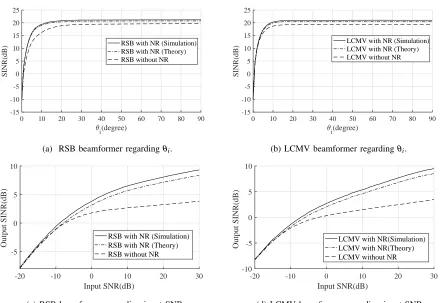
Figure 7: SINR performance of both beamformers with and without the proposed noise reduction (NR) method (M=16,J=100).
array signals are processed by the proposed noise reduction method and then the recovered array signals with an increased
SNR are used as input to the beamformer. The input SNR is 0dB and the TDL lengthJ=100.
The output SINR performances of both beamformers with and without the proposed preprocessing are compared in Fig. 7a
and Fig. 7b as a function of the DOA angle of the interfering signalθi, where the theoretical value is based on the result derived
in Sec. IV. We can see that the simulation result matches the theoretical one very well. With the change of the direction of
the interfering signal, except for the region where DOA of the interfering signal is very close to the desired signal, an almost
constant improvement of about 2dB can be observed.
It is also important to analyse how the SINR performance of the proposed method varies with different input SNRs. Seven
interfering signals are applied to the system, each with a -10dB input SIR, and their DOAs are θi=10◦,20◦,30◦,40◦,50◦,60◦ and 70◦, respectively. All the other settings are the same as before. The results are shown in Fig. 7c and Fig. 7d. As expected, a higher output SINR has been achieved by the proposed method for both beamformers especially when the input SNR is
[image:16.612.83.523.172.475.2]-1 -0.5 0 0.5 1
/
-50 -40 -30 -20 -10 0
[image:17.612.199.401.61.189.2]Gain/[dB]
Figure 8: Frequency response of the row vectors of the 15×15 designed transformation matrix for NLAs.
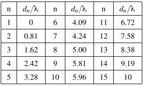
B. Performance of NR method for NLA
These simulations are based on an M=15 NLA example provided in [30], with the sensor locations listed in Table III,
whereλ is the wavelength associated with the normalized frequencyΩ=π. The 15×15 transformation matrix is obtained by
the design procedure described in Sec. V, and its frequency response is shown in Fig. 8. The other settings are the same as
in the ULA case.
n dn/λ n dn/λ n dn/λ
1 0 6 4.09 11 6.72
2 0.81 7 4.24 12 7.58
3 1.62 8 5.00 13 8.38
4 2.42 9 5.81 14 9.19
5 3.28 10 5.96 15 10
Table III: Sensor locations for the wideband NLA example.
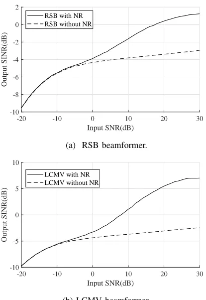
The results are shown in Fig. 9, and we can see that a higher output SINR is achieved by the proposed method for both
beamformers, especially when the input SNR is larger than 0dB and generally the improvement becomes larger when input
SNR increases. However, compared to the ULA case, for input SNR smaller than 0 dB, there is not as much improvement.
After checking the designed transformation matrix, we found that it is far away from being unitary and has a large condition
number, which could be the reason for such a behavior. As mentioned at the end of Sec. V, further research is needed for
designing a unitary transformation matrix for NLAs with the desired frequency responses.
C. Discussion
As can be seen from the proposed structure, we do not need any prior information about the impinging signals to reduce
the noise level and increase the overall SNR by about 3dB. However, although the SNR has been improved, the noise is not
white any more, as specified in (28), whose effect on the ultimate performance of the system can not be seen directly. That is
why we have provided both theoretical analyses and computer simulations to show that indeed by the proposed method, the
performance of the two studied beamformers has been improved.
The above result is obtained from the viewpoint of reducing the noise level of the received signals.
Actually by studying the structure further, it is realised that the proposed structure is equivalent to a traditional TDL system,
[image:17.612.234.378.329.416.2]-20 -10 0 10 20 30
Input SNR(dB)
-10 -8 -6 -4 -2 0 2
Output SINR(dB)
RSB with NR RSB without NR
(a) RSB beamformer.
-20 -10 0 10 20 30
Input SNR(dB)
-10 -5 0 5 10
Output SINR(dB)
LCMV with NR LCMV without NR
[image:18.612.199.406.59.360.2](b) LCMV beamformer.
Figure 9: SINR performance of both beamformers with and without the proposed noise reduction method for the NLA.
to both the original set of array signals and the new set of array signals after the proposed preprocessing, the latter one will
be equivalent to a kind of LCMV beamformer but with much longer TDLs, and hence the improved performance. From this
viewpoint, the proposed method can also be considered as a low-complexity approach to adaptive beamforming. Certainly
another advantage is that the proposed preprocessing is standard and can be applied to the original array signals, whatever the
following processing (either beamforming or DOA estimation, or tracking, etc.) is. As shown in our study for DOA estimation
based on the proposed structure in [13], the improved SNR can be translated into improved DOA estimation performance too.
To show that the overall combination of the proposed noise reduction part and the following TDL-based beamformer is
equivalent to a new beamformer with a much longer TDL, i.e., the noise reduction method alongside the TDL attached can
be modelled as an equivalent TDL with a larger length, we first derive the following result:
y[n] = M−1
∑
k=0 lhp+J−2
∑
n0=0
xk[n−n0] M−1
∑
p=0
apk M−1
∑
m=0 ˜
amp J−1
∑
j=0
wm jhp[n0−j], (59)
wherelhp is the length of the highpass filters and[A−1]mp=a˜mp. By arranging (59), we have:
y[n] = M−1
∑
k=0 lhp+J−2
∑
n0=0
M−1
∑
p=0 M−1
∑
m=0 J−1
∑
j=0
apka˜mpwm jhp[n0−j]xk[n−n0]. (60)
By assuming ˜wk,n0 =∑
M−1
p=0 ∑Mm=0−1∑Jj−=01apka˜mpwm jhp[n0−j], (59) becomes
y[n] = M−1
∑
k=0 lhp+J−2
∑
n0=0
˜
wk,n0xk[n−n0], (61)
-20 -10 0 10 20 30 40 Input SNR(dB)
-10 -5 0 5
Output SINR(dB)
RSB with NR, J=10 RSB without NR, Jeq=110
(a) RSB,J=10 with NR,Jeq=110 without NR.
-20 -10 0 10 20 30 40
Input SNR(dB)
-10 -5 0 5
Output SINR(dB)
LCMV with NR, J=10 LCMV without NR, Jeq=110
(b) LCMV,J=10 with NR,Jeq=110 without NR.
-20 -10 0 10 20 30 40
Input SNR(dB)
-10 -5 0 5 10
Output SINR(dB)
RSB with NR, J=50 RSB without NR, Jeq=150
(c) RSB,J=50 with NR,Jeq=150 without NR.
-20 -10 0 10 20 30 40
Input SNR(dB)
-10 -5 0 5 10
Output SINR(dB)
LCMV with NR, J=50 LCMV without NR, Jeq=150
[image:19.612.77.523.52.367.2](d) LCMV,J=50 with NR,Jeq=150 without NR.
Figure 10: SINR performance of both beamformers with NR method and without NR with equivalent length, lhp=101.
The question here is, since the noise reduction method can be modeled as a TDL, which one of the following gives us a better
performance: using the noise reduction method and a TDL with length Jor using a larger TDL with lengthJeq=lhp+J−1.
We may think the latter one will give a better performance, although it may have the highest implementation complexity,
since a globally optimum solution can be found without constraints imposed by the proposed specific noise reduction process.
However, the real picture is much complicated, due to numerical issues involved in calculating the optimum beamforming
coefficients based on inversion of correlation matrices of difference sizes. The longer the TDL, the larger the dimension of the
matrix involved and the more likely it will cause additional errors in performing matrix inversion.
To show this, again we consider the two types of TDL-based beamformers, i.e., the RSB and the LCMV beamformers. The
SINR performance of both beamformers with the noise reduction method and without the method with the equivalent length
Jeq is shown in Fig. 10. All the simulation conditions are the same as in Section VI-A. When the length of the beamformer is
short (J=10 and equivalent ofJeq=110) as in Fig. 10a and Fig. 10b, the performance of the beamformers without preprocessing
is better, as expected in theory. When the length of the beamformers is larger (J=50 and equivalent of Jeq=150) as in Fig. 10c
and Fig. 10d, the performance of the beamformers with preprocessing is better.
A direct advantage of the proposed noise reduction preprocessing is in reducing the computational complexity of the
beamformers. The computational complexity of the proposed noise reduction method (including the beamforming part), the
directly implemented RSB and LCMV beamformers is presented in Table IV, where N is the number of signal samples at
Algorithm without NR with NR
RSB O(M3J3
eq) +M2Jeq2N+M2Jeq2 +MJeqN O(M3J3) +M2J2N+M2J2+MJN+2M2N+Ml2hp+MNlhp
LCMV O(M3Jeq3) +O(Jeq3) +2M2Jeq3 +2MJeq3 +M2Jeq2N+MJeq2 O(M3J3) +O(J3) +2M2J3+2MJ3+M2J2N+MJ2
+2M2N+Ml2
[image:20.612.75.537.52.108.2]hp+MNlhp
Table IV: Computational complexity of the noise reduction based implementation, the RSB and LCMV beamformers.
VII. CONCLUSION
A method for mitigating the effect of white noise without affecting the directional signals in wideband arbitrary linear arrays
has been introduced. With the proposed method, a maximum 3dB improvement in total signal power to total noise power ratio
(TSNR) can be achieved in the ideal case. A detailed study of the proposed method has been performed and the effect of
the method on the spectra of both the directional signals and in particular white noise is analysed. The increased TSNR can
be translated into performance improvement in various array signal processing applications and as an example, its effect on
beamforming is investigated in detail based on two representative beamformers: the RSB and the LCMV beamformers. As
demonstrated by both theoretical analysis and simulation results, a clear improvement in performance in terms of output SINR
has been achieved.
REFERENCES
[1] H. L. Van Trees,Optimum Array Processing, Part IV of Detection, Estimation, and Modulation Theory. New York: Wiley, 2002.
[2] W. Liu and S. Weiss,Wideband Beamforming: Concepts and Techniques. Chichester, UK: John Wiley & Sons, 2010.
[3] D. Feng, M. Bao, Z. Ye, L. Guan, and X. Li, “A novel wideband DOA estimator based on Khatri–Rao subspace approach,”Signal Processing, vol. 91,
no. 10, pp. 2415–2419, April 2011.
[4] Z. M. Liu, Z. T. Huang, and Y. Y. Zhou, “Direction-of-arrival estimation of wideband signals via covariance matrix sparse representation,” IEEE
Transactions on Signal Processing, vol. 59, no. 9, pp. 4256–4270, Sep. 2011.
[5] Y. D. Zhang, M. G. Amin, F. Ahmad, and B. Himed, “DOA estimation using a sparse uniform linear array with two CW signals of co-prime frequencies,”
inProc. IEEE International Workshop on Computational Advances in Multi-Sensor Adaptive Processing, Saint Martin, December 2013, pp. 404–407.
[6] J. A. Luo, X. P. Zhang, and Z. Wang, “A new subband information fusion method for wideband DOA estimation using sparse signal representation,” in
Proc. IEEE International Conference on Acoustics, Speech, and Signal Processing, Vancouver, Canada, May 2013, pp. 4016–4020.
[7] J. Y. Lee, R. E. Hudson, and K. Yao, “Acoustic DOA estimation: An approximate maximum likelihood approach,”IEEE Systems Journal, vol. 8, no. 1,
pp. 131–141, Mar. 2014.
[8] Y.-S. Yoon, L. M. Kaplan, and J. H. McClellan, “TOPS: new DOA estimator for wideband signals,”IEEE Transactions on Signal Processing, vol. 54,
no. 6, pp. 1977–1989, June 2006.
[9] Q. Shen, W. Liu, W. Cui, S. L. Wu, Y. D. Zhang, and M. Amin, “Low-complexity direction-of-arrival estimation based on wideband co-prime arrays,”
IEEE Trans. Audio, Speech and Language Processing, vol. 23, pp. 1445–1456, September 2015.
[10] B. Widrow, J. R. Glover, J. M. McCool, J. Kaunitz, C. S. Williams, R. H. Hearn, J. R. Zeidler, J. E. Dong, and R. C. Goodlin, “Adaptive noise cancelling:
Principles and applications,”Proceedings of the IEEE, vol. 63, no. 12, pp. 1692–1716, 1975.
[11] T. B. Spalt, C. R. Fuller, T. F. Brooks, and W. Humphreys, “A background noise reduction technique using adaptive noise cancellation for microphone
arrays,” in17th AIAA/CEAS Aeroacoustics Conference, American Institute of Aeronautics and Astronautics, Portland, OR, 2011, pp. 2715–2731.
[12] W. Liu and R. J. Langley, “An adaptive wideband beamforming structure with combined subband decomposition,”IEEE Transactions on Antennas and
Propagation, vol. 89, pp. 913–920, July 2009.
[13] M. R. Anbiyaei, W. Liu, and D. C. McLernon, “Performance improvement for wideband DOA estimation with white noise reduction based on uniform
linear arrays,” inProc. IEEE, Sensor Array and Multichannel Signal Processing Workshop (SAM), Rio de Janeiro, Brazil, July 2016.
[14] R. T. Compton, Jr., “The relationship between tapped delay-line and FFT processing in adaptive arrays,”IEEE Transactions on Antennas and Propagation,
vol. 36, no. 1, pp. 15–26, January 1988.
[15] R. T. Compton, “The bandwidth performance of a two-element adaptive array with tapped delay-line processing,”IEEE Transactions on Antennas and
Propagation, vol. 36, no. 1, pp. 4–14, January 1988.
[16] F. W. Vook and R. T. Compton, Jr., “Bandwidth performance of linear adaptive arrays with tapped delay-line processing,”IEEE Transactions on Aerospace
[17] N. Lin, W. Liu, and R. J. Langley, “Performance analysis of an adaptive broadband beamformer based on a two-element linear array with sensor
delay-line processing,”Signal Processing, vol. 90, pp. 269–281, January 2010.
[18] O. L. Frost, III, “An algorithm for linearly constrained adaptive array processing,”Proceedings of the IEEE, vol. 60, no. 8, pp. 926–935, August 1972.
[19] A. Jakobsson, S. R. Alty, and S. Lambotharan, “On the implementation of the linearly constrained minimum variance beamformer,”IEEE Transactions
on Circuits & Systems II: Express Briefs, vol. 53, no. 10, pp. 1059–1062, October 2006.
[20] W. Liu, S. Weiss, and L. Hanzo, “A subband-selective broadband GSC with cosine-modulated blocking matrix,”IEEE Transactions on Antennas and
Propagation, vol. 52, pp. 813–820, March 2004.
[21] K. Takao and K. Uchida, “Beamspace partially adaptive antenna,”IEE Proceddings H, Microwaves, Antennas and Propagation, vol. 136, pp. 439–444,
December 1989.
[22] T. Sekiguchi and Y. Karasawa, “Wideband beamspace adaptive array utilizing FIR fan filters for multibeam forming,”IEEE Transactions on Signal
Processing, vol. 48, no. 1, pp. 277–284, January 2000.
[23] W. Liu, R. Wu, and R. Langley, “Design and analysis of broadband beamspace adaptive arrays,”IEEE Transactions on Antennas and Propagation,
vol. 55, no. 12, pp. 3413–3420, December 2007.
[24] B. Mulgrew, P. Grant, and J. Thompson, “Random signal analysis,” inDigital Signal Processing. Macmillan Education UK, 1999, pp. 176–205.
[25] R. Bracewell and P. B. Kahn, “The Fourier transform and its applications,”American Journal of Physics, vol. 34, no. 8, pp. 712–712, 1966.
[26] F. Vook and R. Compton Jr, “Bandwidth performance of linear adaptive arrays with tapped delay-line processing,”IEEE Transactions on Aerospace and
Electronic Systems, vol. 28, no. 3, pp. 901–908, 1992.
[27] O. L. Frost III, “An algorithm for linearly constrained adaptive array processing,”Proceedings of the IEEE, vol. 60, no. 8, pp. 926–935, 1972.
[28] Y. Zhao, W. Liu, and R. J. Langley, “An application of the least squares approach to fixed beamformer design with frequency invariant constraints,”IET
Signal Processing, pp. 281–291, June 2011.
[29] B. D. Carlson, “Covariance matrix estimation errors and diagonal loading in adaptive arrays,”IEEE Transactions on Aerospace and Electronic Systems,
vol. 24, pp. 397–401, July 1988.
[30] M. B. Hawes and W. Liu, “Sparse microphone array design for wideband beamforming,” inProc. International Conference on Digital Signal Processing,