This is a repository copy of
The semiparametric asymmetric stochastic volatility model with
time-varying parameters: The case of US inflation
.
White Rose Research Online URL for this paper:
http://eprints.whiterose.ac.uk/141638/
Version: Accepted Version
Article:
Dimitrakopoulos, S (2017) The semiparametric asymmetric stochastic volatility model with
time-varying parameters: The case of US inflation. Economics Letters, 155. pp. 14-18.
ISSN 0165-1765
https://doi.org/10.1016/j.econlet.2017.02.039
© 2017 Elsevier B.V. All rights reserved. Licensed under the Creative Commons
Attribution-Non Commercial No Derivatives 4.0 International License
(https://creativecommons.org/licenses/by-nc-nd/4.0/).
[email protected] https://eprints.whiterose.ac.uk/
Reuse
This article is distributed under the terms of the Creative Commons Attribution-NonCommercial-NoDerivs (CC BY-NC-ND) licence. This licence only allows you to download this work and share it with others as long as you credit the authors, but you can’t change the article in any way or use it commercially. More
information and the full terms of the licence here: https://creativecommons.org/licenses/
Takedown
If you consider content in White Rose Research Online to be in breach of UK law, please notify us by
The semiparametric asymmetric stochastic
volatility model with time-varying parameters:
The case of US inflation
Stefanos Dimitrakopoulos
1Department of Accounting, Finance and Economics, Oxford Brookes University, Oxford,
OX33 1HX, UK
Abstract
We propose a semiparametric extension of the time-varying parameter
re-gression model with asymmetric stochastic volatility. For parameter
estima-tion we use Bayesian methods. We illustrate our methods with an applicaestima-tion
to US inflation.
Keywords: asymmetric stochastic volatility, Dirichlet process, Markov
chain Monte Carlo, time-varying parameters, inflation
JEL CODE: C11, C14, C15, C22
1
1
Introduction
Time varying-parameter regression models with stochastic volatility (TVP-SV
mo-dels) have been successfully applied to inflation modeling (Stock and Watson, 2007;
Clark and Ravazzolo, 2015; Chan, 2017).
In this paper, we focus on the relationship between inflation and volatility that
has been examined by many researchers. (Friedman, 1977) points out the potential
positive association between inflation and volatility. There are also many empirical
evidences, including (Baillie et al., 1996), (Grier and Perry, 1998), and (Fountas,
2001). (Chan, 2017) developed a stochastic volatility in mean model with
time-varying parameters and applied it to estimate inflation. (Chan, 2017) found positive
relationship between inflation and volatility before early 1980s, and zero or even
negative after early 1980s.
The contribution of this paper is threefold. First, we capture the correlation
between inflation and volatility by modeling jointly the distribution of inflation
and log-volatility within a TVP-SV model. Furthermore, the joint distribution
of inflation and volatilities is modelled semiparametrically. The intuition behind
this semiparametric extension is that macroeconomic shocks that have the greatest
effect on the economy are often not symmetric, suggesting that innovations have a
distribution that is skewed to the left or to the right.
(Dimitrakopoulos, 2017) extended semiparametrically the TVP-SV model by
using mixtures of Dirichlet processes (Ferguson, 1973) for the observations’ errors
and the errors of the parameter-driven dynamics. (Dimitrakopoulos, 2017)’s
mix-ture approach over both the mixmix-ture’s means and variances of the observation
dis-tribution can capture this skewness. An alternative flexible approach to capturing
skewness is to jointly model nonparametrically the bivariate distribution of the
ob-servations and the log-volatilities. This approach was proposed by (Jensen and
Ma-heu, 2014) who used a bivariate Dirichlet process mixture model for the innovations
of a SV model with leverage to examine the behaviour of daily returns.
Following (Jensen and Maheu, 2014), we extend the model of (Dimitrakopoulos,
2017) by accounting for a semiparametric asymmetric stochastic volatility that
cap-tures in a flexible way the joint distribution of the empirical skewness of inflation.
The resulting model specification is novel and constitutes our second contribution.
We use Bayesian methods and develop an efficient Markov chain Monte Carlo
algorithm for estimating the parameters of the model. This is our third contribution.
2
Econometric set up
2.1
The TVP-SV model with correlated errors
Consider the following time-varying parameter regression model with asymmetric
stochastic volatility
yt=µ+x′tβ+z′tαt+ exp(ht/2)εt, t= 1, ..., T, (1)
αt+1 =αt+ut, ut ∼N(0,Σ),t = 0,1, ..., T −1, (2)
ht+1 =µh+φ(ht−µh) +ηt,|φ|<1, (3)
where the errors εt and ηt are independently and identically distributed following the bivariate normal distribution,
εt ηt
∼ N
0
0
,
1 ρσh ρσh σh2
. (4)
The parameter-driven dynamics in equation (2) follow a random walk process
which is initialized with α0 = 0 and u0 ∼ N(0,Σ0), for known initial covariance
matrix Σ0.
In equation (3), the term ht is the log-volatility at time t and φ is a persistence parameter that satisfies the stationarity restriction (|φ|<1). The AR(1) stochastic volatility process is initialized withh1 ∼N(µh, σ2h/(1−φ
2
)).
The model given by expressions (1)-(4) is the TVP-SV model with correlated
errors1
(TVP-SVC model). Furthermore, when the correlation parameter ρ equals zero, the TVP-SVC model reduces to the standard TVP-SV model.
We also assume the following priors
β ∼N(β0,B), σ 2
h ∼ IG(va/2, vβ/2), Σ∼IW(δ,∆−1), µh ∼N( ¯µh,σ¯h2), µ ∼N(¯µ,σ¯2), ρ∼N(ρ0, σ
2
ρ)I|ρ|<1,φ ∼N(φ0, σ 2
φ)I|φ|<1,
whereIW and IG denote the Inverse-Wishart distribution and the inverse gamma distribution, respectively. I|ρ|<1 is an indicator function that equals one for the
sta-tionary region and zero otherwise andN(ρ0, σ2ρ)I|ρ|<1 is a normal density truncated
in the stationary region. Similar analysis holds for the prior of φ.
2.2
The semiparametric TVP-SV model with correlated
er-rors
We relax the parametric assumption for the joint distribution ofεtand ηt by letting this distribution be unspecified. To this end, we use the Dirichlet process prior which
is a powerful tool for modelling unknown distributions. For a detailed description
of this prior see (Navarro et al., 2006). 1
In finance, the negative correlation between εtandηtis called leverage effect: as asset prices decline, companies become mechanically more leveraged since the relative value of their debt rises relative to that of their equity. As a result, it is natural to expect that their stock becomes riskier, hence more volatile. It is difficult to imagine that a similar economic argument exists for inflation. For this reason, we avoid using the term “leverage” throughout the paper.
The unspecified functional form of (εt, ηt)′ is given by the following Dirichlet process mixture (DPM) model
εt ηt
|Λt ∼ N(0,Λt),
Λt i.i.d∼ G, G|a, G0 ∼DP(a, G0), (5)
G0 =IW(s0, S0), a∼ G(c, d),
where Λt =
σ2
y,t σyh,t σyh,t σh,t2
. µh in expresson (3) is set to zero for identification
reasons.
Model (5) was first proposed by (Jensen and Maheu, 2014). According to this
model, the conditional distribution of the error vector (εt, ηt)′ given Λt is a bivariate Gaussian with mean zero and random variance-covariance matrix Λt.Λtis generated from an unknown distribution G on which a Dirichlet process prior is imposed. For the prior base distribution G0 we assume an Inverse-Wishart distribution and
for the positive scalar (precision parameter) a we use a gamma prior distribution. Depending on the value ofa, the DPM model in expression (5) can mimic a variety of distributions (bivariate Student-t, bivariate normal, finite mixture of bivariate
normals).
Furthermore, for the distribution ofut we assume the following DPM structure,
ut|ωt,Σ∼N(0, ω−
1
t Σ),t = 1, ..., T −1, ωt
i.i.d
∼ Gω, Gω|aω, G0ω ∼DP(aω, G0ω), (6)
G0ω =G(e2ω,
eω
2 ), aω ∼ G(cω, dω).
mixing variable ωt is generated from a random distribution Gω. G0ω is the prior
baseline gamma distribution andaω is the dispersion parameter. The unconditional distribution of the error ut follows an infinite mixture of multivariate Gaussians, where this mixture arises from the convolution ofGω (the mixing distribution) with a multivariate Gaussian kernel. Due to the clustering property of the Dirichlet process,
this infinite mixture model reduces to a finite mixture of multivariate Gaussians with
a random number of components. The resulting mixture model includes as special
cases the multivariate Student-t and the multivariate Normal.
The TVP-SVC model combined with the DPM models of (5) and (6) produces
the semiparametric TVP-SVC model (S-TVP-SVC model).
3
Posterior analysis
3.1
MCMC algorithm for the S-TVP-SVC model
Our MCMC algorithm updates the parameters (β, h, φ, µ, α, Σ), where h = (h1, ..., hT+1)′ and α = (α1, ...,αT) as well as the DPM parameters. In the Online Appendix we provide details of the MCMC algorithm for the S-TVP-SVC model.
3.2
Density forecasts
We evaluate the performance of the proposed semiparametric model against that of
competing models by conducting a recursive out-of-sample forecasting exercise. In
particular, the comparison of the models is done using density forecasts. Further
details are given in the Online Appendix.
4
Empirical application
4.1
Modeling strategies
Our dataset consists of US quarterly consumer price index (CPI) inflation, covering
the period 1948Q1-2013Q2. The empirical model for capturing inflation dynamics
is an autoregressive TVP-SVC (AR-TVP-SVC) model,
yt=α1,t+α2,tyt−1+ exp(ht/2)εt, t= 1, ..., T,
αt+1 =αt+ut, ut ∼N(0,Σ),
ht+1 =µh+φ(ht−µh) +ηt,|φ|<1,
εt ηt
∼ N
0
0
,
1 ρσh ρσh σh2
,
where yt = 400∗log(lt/lt−1) denotes the CPI inflation and lt is the quarterly CPI figure. We plotyt in Figure 1.
For comparison purposes, we considered three alternative model specifications:
The first model is the the semiparametric version of the AR-TVP-SVC
(AR-S-TVP-SVC) model, where the disturbances (εt, ηt)′ andutfollow the DPM structures of (5) and (6), respectively. The second model is the the AR-S-TVP-SV model, proposed
by (Dimitrakopoulos, 2017) and the third one is the AR-TVP-SVC model, where
the errors (εt, ηt)′ and ut are Student-t distributed. This model is referred to as the AR-St-TVP-SVC model2
.
We threw away the first 100000 draws and kept the next 150000 MCMC draws.
The hyperparameters for the priors of the AR-S-TVP-SVC model are the same as
those used in the simulation experiment of the Online Appendix. 2
4.2
Empirical results
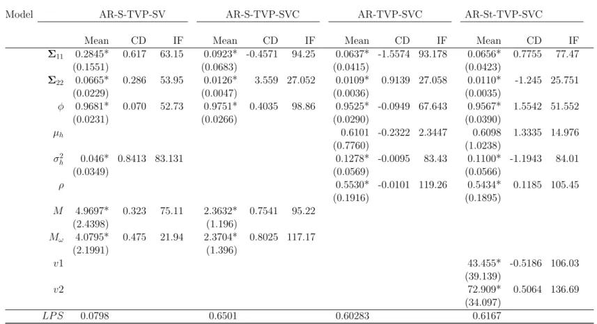
Table 1 presents the estimation results. The posterior estimate of ρ is positive and significant in the parametric models (AR-TVP-SVC and AR-St-TVP-SVC),
with the correlation being stronger in the TVP-SVC model than in the
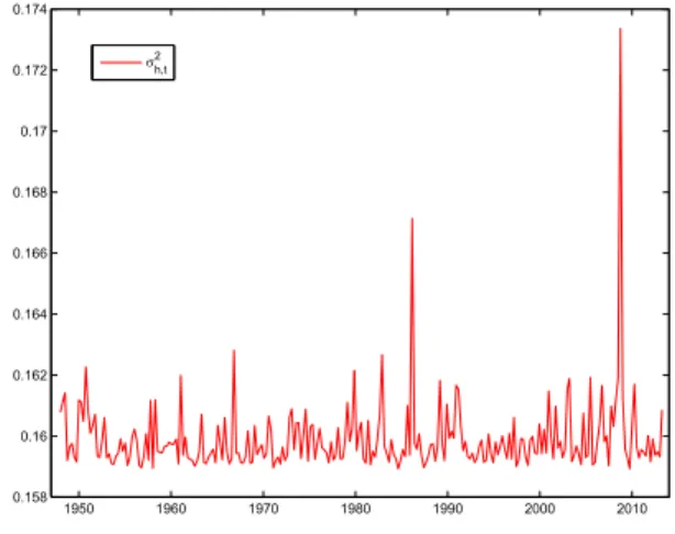
AR-St-TVP-SVC model. The time plot of the expected values ofp(ρt|y1, ..., yT), where ρt = σyh,t/(σy,tσh,t), t = 1, ...,261 obtained from the AR-S-TVP-SVC also shows a positive correlation between inflation and volatility (Figure 2). This correlation
attains its largest values during the period of Great Moderation and the Great
Recession. The same holds for the dynamic evolution of the expected values of
p(σ2
y,t|y1, ..., yT) and p(σh,t2 |y1, ..., yT), t= 1, ...,261 (Figures 3 and 4, respectively). In Table 1, the estimated ρ was found to be large, positive and statistically significant;ρ=0.5434 in the AR-St-TVP-SVC model andρ=0.5530 in the AR-TVP-SVC model. Also, from Figure 2 (AR-S-TVP-AR-TVP-SVC model) the expected values of
ρt are also positive and around 0.4. The positive relationship between inflation and inflation uncertainty has also been supported by previous studies; see for example
(Cukierman and Meltzer, 1986) and (Berument et al., 2009).
In addition, Figure 2 suggests that for the US economy the values of ρt do not fluctuate substantially around 0.4, and therefore the relationship between inflation
and inflation volatility is not time-varying. This empirical finding holds throughout
the period in question and it is in contrast to the empirical findings of (Chan,
2017) for the US economy. (Chan, 2017) proposed a stochastic volatility in mean
model with varying parameters and found that there is a positive and
time-varying relationship between inflation and inflation uncertainty before 1980s, but
no relationship afterward.
Table 1 (last row) reports the density forecast results of the four models. For
the forecasting exercise the evaluation period is from 2013Q3 to 2014Q2. The
AR-S-TVP-SVC model provides better density forecasts than the rest of the models as
this model has the highest log-predictive score3
(LPS). The forecast performance of
the AR-TVP-SVC model is lower than that of the AR-St-TVP-SVC model. The
AR-S-TVP-SV model produces the worst density forecasts. The forecasting results
clearly show that by modeling jointly the distribution of inflation and log-volatility
we substantially improve the forecast performance of the AR-TVP-SV models.
Furt-hermore, these results verify the forecast gains from modeling nonparametrically the
error distributions of the AR-TVP-SVC model.
In Figure 5 the posterior estimates of the coefficientsαtfor the AR-S-TVP-SVC
model exhibit time-variation the path of which is similar to that obtained from the
rest of the models of Table 3 (Figures 6-8).
Additional empirical results are presented in the Online Appendix.
5
Conclusions
Using MCMC methods, we estimated a semiparametric time-varying parameter
re-gression model with asymmetric stochastic volatility. The proposed model had
bet-ter fit to US inflation data than competing models. We also found positive
correla-tion between inflacorrela-tion and log-volatility, volatility fluctuacorrela-tion and time-variacorrela-tion in
coefficients.
3
Table 1: Empirical results
Model AR-S-TVP-SV AR-S-TVP-SVC AR-TVP-SVC AR-St-TVP-SVC
Mean CD IF Mean CD IF Mean CD IF Mean CD IF
Σ11 0.2845* 0.617 63.15 0.0923* -0.4571 94.25 0.0637* -1.5574 93.178 0.0656* 0.7755 77.47
(0.1551) (0.0683) (0.0415) (0.0423)
Σ22 0.0665* 0.286 53.95 0.0126* 3.559 27.052 0.0109* 0.9139 27.058 0.0110* -1.245 25.751
(0.0229) (0.0047) (0.0036) (0.0035)
φ 0.9681* 0.070 52.73 0.9751* 0.4035 98.86 0.9525* -0.0949 67.643 0.9567* 1.5542 51.552
(0.0231) (0.0266) (0.0290) (0.0390)
µh 0.6101 -0.2322 2.3447 0.6098 1.3335 14.976
(0.7760) (1.0238)
σ2
h 0.046* 0.8413 83.131 0.1278* -0.0095 83.43 0.1100* -1.1943 84.01
(0.0349) (0.0569) (0.0566)
ρ 0.5530* -0.0101 119.26 0.5434* 0.1185 105.45
(0.1916) (0.1895)
M 4.9697* 0.323 75.11 2.3632* 0.7541 95.22
(2.4398) (1.196)
Mω 4.0795* 0.475 21.94 2.3704* 0.8025 117.17
(2.1991) (1.396)
v1 43.455* -0.5186 106.03
(39.139)
v2 72.909* 0.5064 136.69
(34.097)
LP S 0.0798 0.6501 0.60283 0.6167
*Significant based on the 95% highest posterior density interval. LPS stands for log-predictive score; see Online Appendix.
1950 1960 1970 1980 1990 2000 2010 -10
-5 0 5 10 15 20
Figure 1: The inflation path from 1948Q1 to 2013Q2
1950 1960 1970 1980 1990 2000 2010 0.38
0.39 0.4 0.41 0.42 0.43 0.44
t
Figure 2: Time plot of the expected value of p(ρt|y1, ..., yT), t = 1, ...,261, obtained from the AR-S-TVP-SVC mo-del.
1950 1960 1970 1980 1990 2000 2010 0.36
0.37 0.38 0.39 0.4 0.41 0.42 0.43
2 y,t
Figure 3: Time plot of the expected value of p(σ2
y,t|y1, ..., yT), t = 1, ...,261, obtained from the AR-S-TVP-SVC mo-del.
1950 1960 1970 1980 1990 2000 2010 0.158
0.16 0.162 0.164 0.166 0.168 0.17 0.172 0.174
2 h,t
Figure 4: Time plot of the expected value of p(σ2
1950 1960 1970 1980 1990 2000 2010 -2 0 2 4 6 8 1t Posterior mean 2SD bands
1950 1960 1970 1980 1990 2000 2010 -1 -0.5 0 0.5 1 2t Posterior mean 2SD bands
Figure 5: Evolution of αt, t = 1, ...,261, obtained from the AR-S-TVP-SVC model; posterior mean (blue), two standard deviation bands (red).
1950 1960 1970 1980 1990 2000 2010 -4 -2 0 2 4 6 8 1t Posterior mean 2SD bands
1950 1960 1970 1980 1990 2000 2010 -1.5 -1 -0.5 0 0.5 1 1.5 2 2t Posterior mean 2SD bands
Figure 6: Evolution of αt, t = 1, ...,261, obtained from the AR-S-TVP-SV model; posterior mean (blue), two standard deviation bands (red).
1950 1960 1970 1980 1990 2000 2010 -2 0 2 4 6 8 1t Posterior mean 2SD bands
1950 1960 1970 1980 1990 2000 2010 -1 -0.5 0 0.5 1 1.5 2t Posterior mean 2SD bands
Figure 7: Evolution of αt, t = 1, ...,261, obtained from the AR-St-TVP-SVC model; posterior mean (blue), two standard deviation bands (red).
1950 1960 1970 1980 1990 2000 2010 -2 0 2 4 6 1t Posterior mean 2SD bands
1950 1960 1970 1980 1990 2000 2010 -1 -0.5 0 0.5 1 1.5 2t Posterior mean 2SD bands
Figure 8: Evolution of αt, t = 1, ...,261, obtained from the AR-TVP-SVC model; posterior mean (blue), two standard deviation bands (red).
References
Baillie RT, Chung CF, Tieslau MA. 1996. Analysing inflation by the fractionally
integrated ARFIMA–GARCH model.Journal of Applied Econometrics11(1): 23– 40.
Berument H, Yalcin Y, Yildirim J. 2009. The effect of inflation uncertainty on
infla-tion: Stochastic volatility in mean model within a dynamic framework. Economic
Modelling 26(6): 1201–1207.
Chan JCC. 2017. The stochastic volatility in mean model with time-varying
para-meters: An application to inflation modeling. Journal of Business & Economic
Statistics 35(1): 17–28.
Clark TE, Ravazzolo F. 2015. Macroeconomic forecasting performance under
alter-native specifications of time-varying volatility. Journal of Applied Econometrics
30(4): 551–575.
Cukierman A, Meltzer AH. 1986. A theory of ambiguity, credibility, and inflation
under discretion and asymmetric information. Econometrica 54(5): 1099–1128.
Dimitrakopoulos S. 2017. Semiparametric Bayesian inference for time-varying
para-meter regression models with stochastic volatility. Economics Letters150: 10–14.
Ferguson TS. 1973. A Bayesian analysis of some nonparametric problems. The
An-nals of Statistics 1(2): 209–230.
Fountas S. 2001. The relationship between inflation and inflation uncertainty in the
UK: 1885–1998. Economics Letters 74(1): 77 – 83.
Friedman M. 1977. Nobel lecture: Inflation and unemployment.Journal of Political
Economy 85(3): 451–472.
Grier KB, Perry MJ. 1998. On inflation and inflation uncertainty in the G7 countries.
Jensen M, Maheu JM. 2014. Estimating a semiparametric asymmetric stochastic
vo-latility model with a Dirichlet process mixture.Journal of Econometrics178: 523– 538.
Navarro DJ, Griffiths TL, Steyvers M, Lee MD. 2006. Modeling individual differences
using Dirichlet processes. Journal of Mathematical Psychology 50(2): 101 – 122.
Stock JH, Watson MW. 2007. Why has U.S. inflation become harder to forecast?
Journal of Money, Credit, and Banking 39: 3–33.
Online Appendix for: The semiparametric asymmetric
stochastic volatility model with time-varying parameters: The
case of US inflation
Stefanos Dimitrakopoulos∗1
1Department of Accounting, Finance and Economics, Oxford Brookes University, UK
1
MCMC algorithm for the S-TVP-SVC model
The estimation of the S-TVP-SVC model is nontrivial, due to the intractability of the like-lihood function under the presence of time-varying parameters, time-varying conditional variances and nonparametric error structures. Our posterior algorithm is as follows:
Posterior sampling of {Λt}
Since Λt,t= 1, ..., T, follows a random discrete probability distribution on which a DP prior is imposed, the set Λ={Λt} will contain m= 1, ..., M,M ≤T unique covariance matrices
Lm, where
Lm=
σy,m2 σyh,m
σyh,m σh,m2
!
,
andM is the number of unique matrices inΛ. DefineL={Lm}andρm=σyh,m/(σy,mσh,m). In addition, let ψ = (ψ1, . . . , ψT)′ be the vector of the latent indicator variables, where
ψt=m when Λt=Lm,m= 1, ..., M.
By introducing ψt in the S-TVP-SVC model, we can orthogonalise the correlated errors
εtand ηt. Following (Jensen and Maheu, 2014), one can show that equations (1) and (3) in the main paper can be rewritten in terms of the orthogonal errorswt and ut as follows
yt=µ+x′tβ+z′tαt+ρψtσy,ψtexp(ht/2)(ht+1−φht)/σh,ψt + exp(ht/2)
q
1−ρ2
ψtσy,ψtwt,wt∼N(0,1),t= 1, ..., T, (A.1)
ht+1=φht+σh,ψtut,|φ|<1,ut∼N(0,1), (A.2)
where (wt, ut) ∼ N(0,I2) and I2 is a 2×2 identity matrix. The posterior sampling of
µ,β,h,α andφ, which is presented below, is based on the equations (A.1) and (A.2).
∗
Let the set Λ(t) denote Λ with Λt removed. Λ(t) will contain M(t) clusters, that is,
L(t) = (L(1t), ..., LM(t)(t))′. The number of matrices in Λ(t) that correspond to the distinct
covariance matrixL(mt) will ben(mt)=Pj1(ψj =m, j6=t),m= 1, ..., M(t).
Instead of simulating Λ, we sample L and ψ to improve mixing (MacEachern, 1994). The sampler for updating{ψt}and {Lm} consists of two steps.
Step 1: Sample eachψt according to the probabilities
P(ψt=m|L(t), ψ(t), n(mt))∝
(
qtm if m= 1, ..., M(t)
qt0 if m=M(t)+1, (A.3)
whereψ(t)=ψ\{ψ
t} and the weightsqt0 and qtm in (A.3) are defined respectively as
qtm∝n(mt)fN(ǫt|0, L(mt)), qt0 ∝a
R
f(ǫt|Λt)dG0(Λt),
whereǫt= (εt, ηt)′ = (yt∗/exp(ht/2), ht+1−φht)′ and yt∗ =yt−µ−x′tβ−z′tαt.
According to (A.3), ψt can take the existing value m= 1, ..., M(t) with probability pro-portional to qtm. In this case, Λt,t= 1, ..., T, is assigned to an existing (unique) covariance matrixL(mt),m= 1, ..., M(t). fN(ǫt|0, L(mt)) is the bivariate normal distribution ofǫtevaluated atL(mt).
Also, according to (A.3),ψt can take a new valuem=M(t)+ 1 with probability propor-tional toqt0. In this case, we set Λt=LM(t)+1and sampleLM(t)+1from the posterior baseline
distribution
Λt|ǫt, S0, s0 ∼IW(s0+ 1, S0+ǫtǫ′t).
The term qt0 is proportional to the dispersion parameter a times an integral which is
the marginal density of ǫt. This density is equal to the bivariate Student-t distribution
qM St(ǫt|0, S0/(s0−1), s0−1), with mean0, covarianceS0/(s0−1) and degrees of freedom
s0−1.
Step 2:
SampleLm,m= 1, ..., M from the following baseline posterior
Lm|{ǫt}t∈Fm, S0, s0∼IW(s0+nm, S0+
X
t∈Fm
ǫtǫ′t),
whereFm={t: Λt=Lm} is the set of Λs equalingLm.
Posterior sampling of a
We sampleaas in (Escobar and West, 1995). So we first sample the latent random variable
ξ from p(ξ|a, M)∼ Beta(a+ 1, T) and then we sample a from a mixture of two gammas,
p(a|ξ, M)∼ πξG(c+M, d−log(ξ))+(1−πξ)G(c+M −1, d−log(ξ)),where πξ/(1−πξ) = (c+M−1)/T(d−log(ξ)).
Posterior sampling of h
Apply the sampler of (Chan, 2017) to the following model
yt=µ+x′tβ+z′tαt+ρψtσy,ψtexp(ht/2)(ht+1−φht)/σh,ψt + exp(ht/2)
q
1−ρ2
ψtσy,ψtwt,wt∼N(0,1), t= 1, ..., T,
ht+1 =φht+σh,ψtut,|φ|<1,ut∼N(0,1).
In particular, one can show that the logarithm of the posterior distribution of the volatil-ity vector h= (h1, ..., hT+1)′ is given by
logp(h|y,β, µ,α,{Λt}, φ)≈const−12(h′Khh−2h′kh) = log g(h), (A.4)
wherey= (y1, ..., yT),Kh=H′Σ−1H+Gand kh=f+Gh˜+H′Σ−1HH−1hˆ. Also, ˆh=
(0, ...,0)′ and Σ =diag(σ2h,0/(1−φ2), σ2h,ψ1, ..., σh,ψ2
T), whereσ
2
h,0=E[G0](2,2) = [s0−Sp0−1](2,2).
The point ˜h is the mode of the posterior logp(h|•) in (A.4). H is a lower triangular sparse matrix H =
1 0 0 · · · 0 −φ 1 0 · · · 0 0 −φ 1 · · · 0
..
. ... ... . .. ... 0 0 · · · −φ 1
.
The gradient vector f = (f1, ..., fT+1)′ and the negative Hessian matrix
G=
G11 G12 0 · · · 0
G21 G22 G23 · · · 0
..
. ... ... . .. ...
0 · · · GT,T−1 GT T GT,T+1
0 · · · 0 GT+1,T GT+1,T+1
,
are calculated as follows:
The logarithm of the conditional distribution p(yt|ht, ht+1,β, µ,αt,Λt, φ) is given by
logp(yt|ht, ht+1,β, µ,αt,Λt, φ) =−12log
2π(1−ρ2ψt)σ2y,ψt-ht
2
− exp(−ht)
2(1−ρ2
ψt)σ2y,ψt
(yt∗−ρψtσy,ψtexp(ht/2) (ht+1−φht)/σh,ψt)
2.
Setting pt = p(yt|ht, ht+1,β, µ,αt,Λt, φ) for notational convenience, we have for t = 2, ..., T + 1,
G11=−d
2logp
t dh2
t , Gtt =− d2(logp
t+logpt−1)
dh2
t , Gt−1,t=− d2logp
t dhtdht+1,
evaluated ath= ˜h, where
dlogpt dht =−
1
2 −2(1−1ρ2
ψt)
− y2t∗ σ2
y,ψtexp(ht)− 2ρ2
ψtφ(ht+1−φht)/σ
2
h,ψt
+ y
∗ tρψt
σy,ψtexp(ht/2)σh,ψt(ht+1−φht+ 2φ)
,
d2logp
t dh2
t =−
1 2(1−ρ2
ψt)
y2∗ t σ2
y,ψtexp(ht) + 2ρ2ψ
tφ
2/σ2
h,ψt
− y∗tρψt
2σy,ψtexp(ht/2)σh,ψt (ht+1−φht+ 4φ)
,
dlogpt dht+1 =−
1 (1−ρ2
ψt)
ρ2ψt(ht+1−φht)/σh,ψ2 t − y
∗ tρψt σy,ψtexp(ht/2)σh,ψt
,
d2logp
t dh2
t+1 = −
ρ2
ψt
(1−ρ2
ψt)σh,ψt2 ,
d2logp
t dhtht+1 =−
1 (1−ρ2
ψt)
ρ2
ψtφ/σ
2
h,ψt −
y∗ tρψt
2σy,ψtexp(ht/2)σh,ψt
.
According to expression (A.4), the posterior p(h|y,β, µ,α,{Λt}, φ) is approximated by a Gaussian g(h) ∝ N(mˆ,Kh−1), with mean mˆ = Kh−1kh and precision matrix Kh.
This Gaussian approximation is used as a proposal density in the Acceptance-Rejection Metropolis-Hastings algorithm (see, for example, (Tierney, 1994) and (Chib and Greenberg, 1995)), where candidate draws are obtained using the precision sampler of (Chan and Jeli-azkov, 2009), instead of Kalman-filter based methods.
The precision sampler of (Chan and Jeliazkov, 2009) works as follows. First of all, note thatKhis a sparse matrix and therefore we can compute fast and efficientlymˆ without the
need to obtain the inverseKh−1, which involves a time-consuming matrix operation due to
its large size. Instead, we solve the linear systemKhmˆ =kh. Next, we obtain the Cholesky
decomposition Kh = CC′. Let x = C−1z, where z ∼ N(0,I). Then, x ∼ N(0,Kh−1).
Finally return m˜ =mˆ +x.
Posterior sampling of β
Updateβ by sampling from
β|B,β0, µ,α,h, φ,y,{Λt} ∼N(D0d0, D0),
where
D0 =
B−1+PT
t=1
xtx′ t
exp(ht)σy,ψt2 (1−ρ2ψt)
−1
,
d0 =B−1β0+
T
P
t=1
xt(yt−µ−z′tαt−ρψtσy,ψtexp(ht/2)(ht+1−φht)/σh,ψt)
exp(ht)σy,ψt2 (1−ρ2ψt) .
Posterior sampling of µ
Updateµ by sampling from
µ|µ,¯ σ¯2,α,β,h, φ,y,{Λ
t} ∼N(D1d1, D1),
where
D1 =
1 ¯
σ2 +
T
P
t=1
1
exp(ht)σy,ψt2 (1−ρ2ψt)
−1
,
d1 = ¯σµ¯2 +
T
P
t=1
yt−x′tβ−z′tαt−ρψtσy,ψtexp(ht/2)(ht+1−φht)/σh,ψt
exp(ht)σ2y,ψt(1−ρ2ψt) .
Posterior sampling of φ
We update φ using an independence Metropolis-Hastings algorithm. In particular, at the
l −th iteration we draw a candidate value φ(p) from the truncated normal distribution
N(σ2ˆ
φφ, σˆ
2 ˆ
φ)I|φ|<1, where
σ2ˆ
φ=
1
σ2
φ +PT
t=1
h2
t σ2
h,ψt +PT
t=1
ρ2
ψth2t σ2
h,ψt(1−ρ2ψt)
−1 , ˆ φ= φ0 σ2 φ +PT
t=1
htht+1
σ2
h,ψt +PT
t=1
ρψtht(y∗t−ρψtht+1σy,ψtexp(ht/2)/σh,ψt) σh,ψtσy,ψtexp(ht/2)(1−ρ2ψt)
−1
.
Given φ(p) and the value from the previous iteration φ(l−1), φ(p) is accepted as a valid current draw (φ(l)=φ(p)) with probability
ap(φ(l−1), φ(p)) = min(
f(h1|σh,20,φ(p))
f(h1|σh,20,φ(l−1)) ,1),
wheref(h1|σh,20, φ) =N(0, σh,20/(1−φ2)).
Posterior sampling of α
Apply the precision sampler of Chan and Jeliazkov (2009) to the following model
˜
yt=z′tαt+ exp(ht/2)
q
1−ρ2
ψtσy,ψtwt,wt∼N(0,1), t= 1, ..., T,
αt+1 =αt+ut,ut ∼N(0, ωt−1Σ), t= 0,1, ..., T −1,
where ˜yt=yt−µ−x′tβ−ρψtσy,ψtexp(ht/2)(ht+1−φht)/σh,ψt. In particular, stacking the equation for ˜yt overt= 1, ..., T,we have
˜
y=Zα+ξ,ξt∼N(0,Sy)⇔
Z=
z′1 0 0 · · · 0 0 z′2 0 · · · 0 0 0 z′3 · · · 0
..
. ... ... . .. ... 0 0 0 · · · z′T
,Sy˜=
s1 0 0 · · · 0
0 s2 0 · · · 0
0 0 s3 · · · 0
..
. ... ... . .. ... 0 0 0 · · · sT
,
and st= exp(ht)(1−ρ2ψt)σy,ψ2 t,t= 1, ..., T.
The state equation αt+1 =αt+ut,can be written in a matrix notation as follows,
Γα=δ˜α+u,u∼N(0,Su),
whereδ˜α= (α0,0, ...,0)′,u= (u0,u1, ...,uT−1)′,Su =diag(Σ0, ω1−1Σ, ..., ω−T−11Σ) and Γ is
the first difference matrix
Γ=
Ip 0 0 · · · 0 −Ip Ip 0 · · · 0 0 −Ip Ip · · · 0
..
. ... ... . .. ... 0 0 · · · −Ip Ip
.
Hence, the prior distribution of α is a normal distribution, that is, α|{ωt}Tt=1−1,Σ ∼
N(δα,(Γ′S−u1Γ)−1), where δα=Γ−1δ˜α. The posterior distribution of αis also normal
α|{ωt}Tt=1−1,Σ,y˜∼N(αˆ,D−α1),
where
Dα=Γ′S−u1Γ+Z′S−y˜1Z,
ˆ
α=D−α1(Γ′S−u1Γδα+Z′S−y˜1y˜).
Note that Dα is a high-dimensional covariance matrix and therefore sampling from this
posterior can be time-consuming. However, Dα is a band matrix and we can sample from N(αˆ,D−α1) efficiently and fast, using the precision sampler of Chan and Jeliazkov (2009) which is based on block-banded and sparse matrix algorithms and not on Kalman-filter re-lated methods.
Posterior sampling of Σ UpdateΣby sampling from
Σ|δ,∆,α,ω∼IW
δ+T −1,∆−1+TP−1
t=1
ωt(αt+1−αt)(αt+1−αt)′
,
whereω= (ω1, ..., ωT−1).
Posterior sampling of ω
Having calculatedutfromut=αt+1−αt, t= 1, ..., T−1, we updateωas in (Dimitrakopou-los, 2017). Since ωt,t= 1, ..., T−1 follows the Dirichlet process prior Gω, realizations ofωt from Gω will lie in a set ofMω≤T−1 distinct values or clustersω∗ = (ω∗1, ..., ω∗Mω), where
ωm∗ω,mω= 1, ..., Mω is a random draw from G0ω.
Let ω(t) denote all the elements in {ωt}Tt=1−1 excluding the component ωt. The vector
ω(t) will contain ties. Suppose that ω(t) contains Mω(t) unique values, (ω1∗(t), ..., ω
∗(t)
Mω(t) ) and
assume also that each of these values appears in ω(t),n(mt)ω times, wheren
(t)
mω =
P
j1(ψjω =
mω, j 6=t),mω= 1, ..., Mω(t). The termψωt,t= 1, ..., T−1 is a latent indicator variable such that ψtω=mω whenωt=ω∗mω,mω = 1, ..., Mω.
From the P´olya-urn process (Blackwell and MacQueen, 1973), one can easily show that {ωt}Tt=1−1 can be updated from the conditional posterior (continuous-discrete) distribution
p ωt|ω(t),ut, eω,Σ, G0ω
∝q˜t0p(ωt|ut, eω,Σ) + Mω(t)
X
mω=1 ˜
qtmωδω∗(t)
mω(ωt),
t= 1, ..., T−1, (A.5)
where the posterior density ofωtunder the prior G0ω is a gamma density, namely
p(ωt|ut, eω,Σ)∝p(ut|Σ, ωt)G0ω(ωt)∝ω eω+p
2 −1
t e− ωt(eω+u′
tΣ−1ut)
2 ,
and the weights ˜qt0and ˜qtmωare given respectively by ˜qt0∝a
R
f(ut|Σ)dG0ω(ωt)∝aqt(ut|0,Σ, eω), whereqtdenotes the multivariate t-density function, and ˜qtmω ∝n
(t)
mωfN(ut|0, 1
ω∗mω(t)Σ), where
fN denotes the multivariate normal distribution.
We do not sample directly from expression (A.5) but instead update the latent indicators in an analogous way to that for Λs and resample the clustersω∗
mω,mω = 1, ..., Mω from the posterior gamma distribution
p(ω∗mω|{ut}t∈Fmω, eω,Σ)∝ω
∗
mω
eω+p×nmω
2 −1e−
ωmω∗ (eω+ P
t∈Fmω
u′
tΣ−1ut)
2 ,
whereFmω ={t:ωt=ωm∗ω} is the set of ωs sharing the parameter ω
∗
mω.
Posterior sampling of aω
We updateaω in the same way we update a.
2
Density forecasts
Forecast evaluation is conducted in terms of density forecasts. Define ΩT = (y,XT,ZT), wherey= (y1, ..., yT),XT = (x1, ...,xT) andZT = (z1, ...,zT).
GivenΩT andG(the prior baseline distribution), we compute the one-step-ahead out-of-sample predictive density of yT+1,f(yT+1|G,ΩT), which is used as the density forecast for
of the predictive likelihood, which is the logarithm of the predictive density evaluated at the observed yTo+1, namely, f(yTo+1|G,ΩT). Next, we move one period forward and repeat the same forecasting exercise using ΩT+1 data. For the evaluation period t= T + 1, ..., T +k,
the sum of the log predictive likelihoods PT+k−1
t=T logf(yto+1|G,ΩT) is known as the log predictive score of the model. Higher values entail better (out-of-sample) forecasting ability of the model.
The predictive densityf(yT+1|G,ΩT) is obtained as follows. LetΘdenote the parameter vector of the model, that is, Θ=(β, Σ, α, h, φ, µ Λ,ω, a, aω)′, where Λ = {Λt} and ω = (ω1, ..., ωT−1). For the S-TVP-SVC model the (one-step ahead) joint predictive density of
f((yT+1, hT+2)′) conditional on the prior baseline distributionGand on the dataΩT is given by
f yT+1 hT+2 |
G,ΩT
!
=
Z
f yT+1 hT+2 |
Θ
!
π(Θ|ΩT)dΘ, (A.6)
withGhaving been integrated out of the distribution of the error vector (εt,ηt)′. Expression (A.6) is approximated via Monte Carlo simulation by
f yT+1 hT+2 |
G,ΩT
!
≈ L1 L
X
l=1
ˆ
f yT+1 hT+2 |
Θ(l)
!
, (A.7)
where the functional form of the density in the right hand side of expression (A.7) is given by
f yT+1 hT+2 |
Θ
!
= a
a+TfM St
yT+1
hT+2
!
; µ+x
′
T+1β+z′T+1αT+1
φhT+1
!
,ET+1S0ET+1 s0−1
, s0−1
!
+ 1
a+T
M
X
m=1
nmN
yT+1
hT+2
!
; µ+x
′
T+1β+z′T+1αT+1
φhT+1
!
, ET+1LmET+1
!
,
wherefM St(r1, r2, r3) is the bivariate Student-t distribution with meanr1, covariancer2and
degrees of freedom r3, αT+1 is obtained from equation (2) of the manuscript and ET+1 =
exp(h(T+1)/2) 0
0 1
!
. Lis the number of iterations (after the burn-in period).
From expression (A.6) we can obtain the marginal posterior predictive density of yT+1,
which is defined as
f(yT+1|G,ΩT) =
Z
f(yT+1|Θ)f(Θ|ΩT)dΘ≈ 1 L L X l=1 ˆ
f(yT+1|Θ(l)),
where ˆf(yT+1|Θ(l)) when evaluated at an observed valueyT+1 is the predictive likelihood of
the S-TVP-SVC model and is defined as
f(yT+1|Θ) = a
a+TfSt(yT+1;µ+x
′
T+1β+z′T+1αT+1,
S0(1,1)exp(h(T+1)) s0−1
, s0−1)
+ 1
a+T
M
X
m=1
nmN(yT+1;µ+x′T+1β+z′T+1αT+1,exp(h(T+1))σy,m2 ),
wherefStis the univariate Student-t distribution with meanµ+x′T+1β+z′T+1αT+1, variance
S0(1,1)exp(h(T+1))
s0−1 and degrees of freedoms0−1. S0(1,1) is the (1,1) element of S0.
3
The St-TVP-SVC model
Consider the following TVP-SV model,
yt=µ+x′tβ+z′tαt+ exp(ht/2)√λ1tεt,t= 1, ..., T,
αt+1=αt+ut,ut∼N(0, λ−2t1Σ),
ht+1 =µh+φ(ht−µh) +ηt,|φ|<1,
εt
ηt
!
∼ N
"
0 0
!
, 1 ρσh ρσh σ2h
!#
,
where λ1t ∼ IG(v1/2, v1/2), λ2t ∼ G(v2/2, v2/2) and v1 and v2 follow a uniform prior on the domain [3, 120].
To update v1 and v2 we use Metropolis-Hastings steps.
4
Monte Carlo experiments
To evaluate the efficiency of the proposed MCMC algorithm for the semiparametric TVP-SVC model we conducted Monte Carlo experiments.
The simulated data set was generated from the following model
yt= 0.2 +x′tβ+z′tαt+ exp(ht/2)√λtεt,λt∼ IG(8/2,8/2),t= 1, ...,260,
αt+1 =αt+ut,ut∼M V t(0,Σ,5),
ht+1= 0.8ht+ηt,
εt
ηt
!
∼ N
"
0 0
!
, 1 −0.5×
√ 0.1 −0.5×√0.1 0.1
!#
where β = (−1,3)′, α
t = (α1t, α2t)′ and ρ = −0.5. M V t is the multivariate-t distribution with mean 0, covariance matrix Σ = diag(2,2) and degrees of freedom 5, where diag(·) denotes a diagonal matrix. Also,α1 = (−10,20)′. T = 260 is almost equal to the size of the
empirical data set.
The elements of xt = (x1t, x2t)′ and zt = (z1t, z2t)′ for t = 1, ..., T are drawn from a uniform distribution, that is, xjt ∼U(−0.5,0.5) and zit ∼U(−0.5,0.5) forj, i= 1,2.
We assume the following prior distributions
β∼N(0,20×I2×2), α1∼N(0,10×I2×2), µ∼N(0,10),
φ∼N(0.97,0.12)I|φ|<1,Σ∼IW(1,10×I2×2),G0=IW(10, I2×2),
G0ω=G(52,52),a∼ G(3,9), aω ∼ G(3,9),
whereI2×2 is a 2×2 identity matrix.
After discarding the first 50000 draws, we run the sampler 150000. The code was written in Matlab and run on a desktop with an Intel Core i7-4710HQ @2.50 GHz 2.50 GHz. For
T = 260, it takes about 1091 seconds for 10000 iterations.
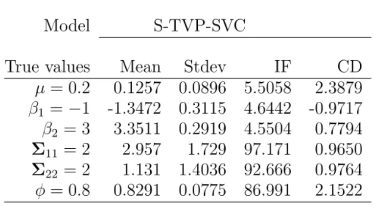
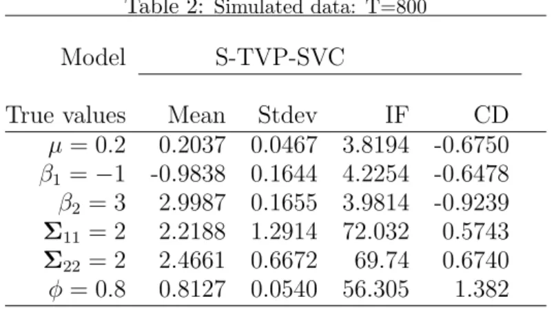
In Table 1 we present the posterior means and standard deviations of the model param-eters. We also report the CD statistics of (Geweke, 1992) and the inefficiency factor (IF); see, for example, (Chib, 2001). Given the small sample size (T = 260), the sampler of the S-TVP-SVC model leads to satisfactory estimation accuracy. This accuracy improves as the sample size increases; in Table 2 we present the estimation results, using the same simulated data set but for T = 8001.
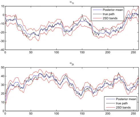
Furthermore, Figures 1 (T = 260) and 2 (T = 800) show the evolution of the estimated time-varying parameters α1t and α2t, along with their two standard deviation bands. The semiparametric model is able to capture the time variation of the coefficients, with their estimated posterior means tracing well the true path of the states.
Table 1: Simulated data: T=260
Model S-TVP-SVC
True values Mean Stdev IF CD
µ= 0.2 0.1257 0.0896 5.5058 2.3879
β1 =−1 -1.3472 0.3115 4.6442 -0.9717
β2 = 3 3.3511 0.2919 4.5504 0.7794
Σ11= 2 2.957 1.729 97.171 0.9650
Σ22= 2 1.131 1.4036 92.666 0.9764
φ = 0.8 0.8291 0.0775 86.991 2.1522
1For
T = 800, it takes about 3319 seconds for 10000 iterations.
0 50 100 150 200 250 -40
-30 -20 -10 0 10
1t
Posterior mean true path 2SD bands
0 50 100 150 200 250
0 10 20 30 40 50
2t
Posterior mean true path 2SD bands
Figure 1: Simulated data: Path of the estimated α1t and α2t for the S-TVP-SVC model; T=260. True path (black), posterior mean (blue), two standard deviation bands (red).
0 100 200 300 400 500 600 700 800
-40 -20 0 20 40
1t
Posterior mean true path 2SD bands
0 100 200 300 400 500 600 700 800
0 20 40 60 80
2t
Posterior mean true path 2SD bands
Table 2: Simulated data: T=800
Model S-TVP-SVC
True values Mean Stdev IF CD
µ= 0.2 0.2037 0.0467 3.8194 -0.6750
β1 =−1 -0.9838 0.1644 4.2254 -0.6478
β2 = 3 2.9987 0.1655 3.9814 -0.9239
Σ11= 2 2.2188 1.2914 72.032 0.5743
Σ22= 2 2.4661 0.6672 69.74 0.6740
φ = 0.8 0.8127 0.0540 56.305 1.382
5
Additional empirical results
In Table 1 of the main paper, the DMP structure of expression (5) for the AR-S-TVP-SVC model produced M = 2.3632 clusters (M is explained in this Online Appendix). In other words, the proposed semiparametric model requires 2.3632 bivariate Gaussians to fit the data. For the AR-S-TVP-SV model, the estimated value of M was larger (M = 4.3697) to that of the AR-S-TVP-SVC model. Similarly, the AR-S-TVP-SV and AR-S-TVP-SVC models gave different degree of clustering, Mω, in ω = (ω1, ..., ωT−1). Mω is also explained in this Online Appendix. The nonnormality of the errors (εt, ηt)′ and ut is also supported by the reported values of the degrees of freedom for the AR-St-TVP-SVC model (see Table 1 of the main paper).
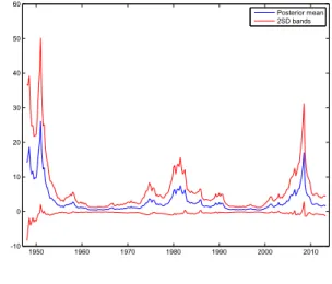
In Figures 3-6 of this Appendix, we present the posterior mean of the time-varying volatility for the four empirical models of the main paper. This posterior mean is smoother in Figure 3 than in Figures 4 and 5. In Figure 6, the posterior estimates of volatilities for the AR-S-TVP-SVC model are much larger than those for the rest of the models. This is justified by the large expected values of p(σ2
h,t|y1, ..., yT), t = 1, ...,261; see Figure 4 of the main paper.
1950 1960 1970 1980 1990 2000 2010 -20
-10 0 10 20 30 40 50
Posterior mean 2SD bands
Figure 3: Evolution of exp(ht), t = 1, ...,261, obtained from the AR-S-TVP-SV model; posterior mean (blue), two standard deviation bands (red).
1950 1960 1970 1980 1990 2000 2010 -10
0 10 20 30 40 50 60
Posterior mean 2SD bands
Figure 4: Evolution of exp(ht), t = 1, ...,262, obtained from the AR-TVP-SVC model; posterior mean (blue), two standard deviation bands (red).
1950 1960 1970 1980 1990 2000 2010 -10
0 10 20 30 40 50
Posterior mean 2SD bands
Figure 5: Evolution of exp(ht), t = 1, ...,262,obtained from the AR-St-TVP-SVC model; posterior mean (blue), two standard deviation bands (red).
1950 1960 1970 1980 1990 2000 2010 -50
0 50 100 150 200 250
Posterior mean 2SD bands
References
Blackwell D, MacQueen J. 1973. Ferguson distributions via p´olya urn schemes. The Annals of Statistics 1(2): 353–355.
Chan JCC. 2017. The stochastic volatility in mean model with time-varying parameters: An application to inflation modeling.Journal of Business & Economic Statistics35(1): 17–28.
Chan JCC, Jeliazkov I. 2009. Efficient simulation and integrated likelihood estimation in state space models. International Journal of Mathematical Modelling and Numerical Op-timisation 1: 101–120.
Chib S. 2001. Markov Chain Monte Carlo methods: Computation and Inference.In Heckman JJ. and Leamer E, (Eds.), Handbook of Econometrics, Volume 5, (pp. 3569-3649). Elsevier.
Chib S, Greenberg E. 1995. Understanding the Metropolis–Hastings algorithm.The Ameri-can Statistician 49(4): 327–335.
Dimitrakopoulos S. 2017. Semiparametric Bayesian inference for time-varying parameter regression models with stochastic volatility.Economics Letters 150: 10–14.
Escobar M, West M. 1995. Bayesian density estimation and inference using mixtures.Journal of the American Statistical Association 90(430): 577–588.
Geweke J. 1992. Evaluating the Accuracy of Sampling-Based Approaches to the Calculation of Posterior Moments. In Bernardo J, Berger J, Dawid A and Smith A, (Eds.), Bayesian Statistics 4, Oxford: Clarendon Press, (pp. 641-649).
Jensen M, Maheu JM. 2014. Estimating a semiparametric asymmetric stochastic volatility model with a Dirichlet process mixture. Journal of Econometrics178: 523–538.
MacEachern SN. 1994. Estimating normal means with a conjugate style Dirichlet process prior. Communications in Statistics. Simulation and Computation 23(3): 727–741.
Tierney L. 1994. Markov Chains for exploring posterior distributions.The Annals of Statis-tics 22(4): 1701–1728.