This is a repository copy of Measures on mixing angles.
White Rose Research Online URL for this paper:
http://eprints.whiterose.ac.uk/151734/
Version: Accepted Version
Article:
Gibbons, G.W., Gielen, S. orcid.org/0000-0002-8653-5430, Pope, C.N. et al. (1 more
author) (2009) Measures on mixing angles. Physical Review D, 79 (1). ISSN 2470-0010
https://doi.org/10.1103/physrevd.79.013009
© 2009 American Physical Society. This is an author-produced version of a paper
subsequently published in Physical Review D. Uploaded in accordance with the publisher's
self-archiving policy.
[email protected] Reuse
Items deposited in White Rose Research Online are protected by copyright, with all rights reserved unless indicated otherwise. They may be downloaded and/or printed for private study, or other acts as permitted by national copyright laws. The publisher or other rights holders may allow further reproduction and re-use of the full text version. This is indicated by the licence information on the White Rose Research Online record for the item.
Takedown
If you consider content in White Rose Research Online to be in breach of UK law, please notify us by
arXiv:0810.4813v3 [hep-ph] 13 Jan 2009
Measures on Mixing Angles
Gary W. Gibbons
1, Steffen Gielen
1, C. N. Pope
1,2and Neil Turok
1,31
D.A.M.T.P., Centre for Mathematical Sciences, Cambridge University,
Wilberforce Road, Cambridge, CB3 0WA, U.K.
2
George P. & Cynthia W. Mitchell Institute for Fundamental Physics and Astronomy,
Texas A&M University, College Station, TX 77843-4242, USA
3
Perimeter Institute for Theoretical Physics,
31 Caroline St. N., Waterloo, Ontario, Canada N2L 2Y5
October 24, 2018
Abstract
We address the problem of the apparently very small magnitude of CP violation in the
stan-dard model, measured by the Jarlskog invariantJ. In order to make statements about
probabili-ties for certain values ofJ, we seek to find a natural measure on the space of Kobayashi-Maskawa
matrices, the double quotient U(1)2
\SU(3)/U(1)2
. We review several possible, geometrically
motivated choices of the measure, and compute expectation values for powers ofJfor these
mea-sures. We find that different choices of the measure generically make the observed magnitude of
CP violation appear finely tuned. Since the quark masses and the mixing angles are determined
by the same set of Yukawa couplings, we then do a second calculation in which we take the
known quark mass hierarchy into account. We construct the simplest measure on the space of
3×3 Hermitian matrices which reproduces this known hierarchy. Calculating expectation values
for powers ofJin this second approach, we find that values ofJclose to the observed value are
now rather likely, and there does not seem to be any fine-tuning. Our results suggest that the
choice of Kobayashi-Maskawa angles is closely linked to the observed mass hierarchy. We close
by discussing the corresponding case of neutrinos.
Contents
1 Introduction 3
1.1 Geometric Probability . . . 5
1.2 CP Violation and the Jarlskog Invariant . . . 6
2 Metrics on SU(3) and its Quotients 8 2.1 The flag manifoldSU(3)/U(1)2 . . . . 10
2.2 Kaluza-Klein reduction of the bi-invariant metric . . . 12
2.3 Squashed Kaluza-Klein metrics . . . 14
2.4 Ozsv´ath-Sch¨ucking metric . . . 14
3 Statistics of the Jarlskog Invariant J 16 3.1 The flag-manifold measure . . . 16
3.2 The Kaluza-Klein measure from the bi-invariant metric . . . 18
3.3 The Kaluza-Klein measure from squashed metrics . . . 18
3.4 The Ozsv´ath-Sch¨ucking measure . . . 19
3.5 The uniform measure . . . 19
4 Fine-tuning of J 20 4.1 Probability distribution ofJ . . . 20
4.2 Wolfenstein parametrization . . . 22
5 Quark Mass Matrices and Gaussian Weighting Functions 23 5.1 Distributions on Hermitian matrices . . . 23
5.2 Results and dependence on quark masses . . . 27
6 Extension to Neutrinos 32 6.1 Neutrino masses . . . 32
6.1.1 The Universality of free fall . . . 34
6.2 Neutrino mixing matrix . . . 36
6.3 Statistics of J . . . 36
1
Introduction
A traditional attitude to theoretical physics has been that the main problem is to discover the
fundamental laws of physics and leave it to experiment and observation to decide what particular
implementation best describes “Our Universe.” Thus traditionally a “physical theory” is often
thought of in terms of a local Lagrangian including certain “coupling constants,” “mass ratios,” and
“mixing angles,” all of which, since Planck’s introduction of Planck units [1], may be taken to be
dimensionless numbers. In addition, the local Lagrangian must be supplemented with an account of
the general class of boundary conditions for which the variational principle is valid. Different classes
of boundary conditions are usually thought of as different “superselection sectors” of the theory, and
describe qualitatively different types of situations which traditionally are not thought of as having
any relation to one another.
Within each sector, there are many solutions of the equations of motion, each of which may be
specified by providing suitable “initial conditions.” Classically these conditions may be thought of
as the space of classical histories, and given in terms of Cauchy data modulo the relation that two
sets of Cauchy data giving the same history are taken to be equivalent. Quantum mechanically one
thinks in terms of some initial, and thus in the Heisenberg picture, eternal state.
The hope has frequently been expressed in the past that eventually theorists will hit upon a
unique theory, with all coupling constants determined by consistency or symmetry considerations,
and with just one superselection sector. Even given such a “theory of everything” (TOE), there
remains the issue of boundary conditions or initial state, as emphasized by Hawking [2]. Recently,
however, there has been a considerable decline in optimism and few now seem to believe in a single
TOE with a single superselection sector, and many refer to a “landscape” of theories.
One approach to this perceived crisis in theoretical physics is to resort to “anthropic”
considera-tions and invoke the idea that there may indeed exist, in the Platonic sense, an enormous number of
“possible universes,” of which only very few will allow the development of sentient beings, and even
fewer will allow sentient beings like ourselves. Thus one is led to contemplate the ensemble of all
pos-sible universes, sometimes referred to as a “multiverse” [3]. This ensemble is sometimes thought of
non-Platonically1as an ensemble of connected subsets of a much bigger physically existing universe,
referred to as a meta-universe [4].
At this point it may be helpful to remark, lest the daunting task of thinking about and making
more precise, the nebulous notion of such a multiverse should not be thought entirely a problem for
theorists seeking credit for making predictions about the world we see about us: that the observers
and experimenters must also face up to that task when assessing the reliability of their measurements
or the extent to which they can confirm theoretical predictions. All such activities are essentially
Bayesian in character [5] and require some notion of “priors,” that is, some sort ofa priorimeasure
of the space of possibilities.
This problem has been addressed, with admittedly only partial success, in a previous paper [6]
1
where the multiverse, for concreteness, was identified with the set of classical histories of a
min-isuperspace cosmological model. A well-defined and natural local measure on the space of classical
histories is easily constructed, but unfortunately the total measure of all histories, even in this
finite-dimensional truncation of the full set of solutions of Einstein’s equations, is infinite. The problem
was recently revisited in [7].
In the present paper, we shall turn to the problem of finding a natural measure on the space of
coupling constants. Thus the multiverse in the present paper is a set of Lagrangians parametrized
by a manifold X or “moduli space,” whose coordinates consist of masses, mixing angles, coupling
constants, etc., and we wish to place a natural measure on this space. We hope this will be useful
for anthropic considerations such as those of [8], whereX ≡S1, the circle parametrizing the phase
of the axion. In that case the issue of a measure was trivial, but in more complicated cases such
as we shall consider in the present paper, the situation is more complicated. We also hope that
the work in this paper will help in clarifying the notion of “fine-tuning,” which is so prevalent in
phenomenological discussions.
The structure of this paper is as follows. After introducing the notion of geometric probability and
outlining the Kobayashi-Maskawa theory of CP violation in the standard model, we discuss metrics
onSU(3) and its quotients in Sec. 2, starting with a left-invariant metric onSU(3) which induces
a metric on the flag manifoldSU(3)/U(1)2. We perform a Kaluza-Klein type reduction on the left
phases and discuss different possible metrics on the double quotientU(1)2\SU(3)/U(1)2, the space
of Kobayashi-Maskawa matrices. We also discuss the metric used by Ozsv´ath and Sch¨ucking [9],
and argue that it lacks a geometrical justification.
We then use all metrics we have discussed to compute statistics of the Jarlskog invariantJ. While
the measure onSU(3)/U(1)2 is independent from the choice of left-invariant metric, the measure
on the double quotient is nonunique. We find that in each case the standard deviation ∆J (with
hJi = 0) is about three orders of magnitude greater than the experimentally observed value ofJ,
which appears to be finely tuned. In Sec. 4, we do a closer numerical analysis of the probability
distribution of|J|on the double quotient, using several possible choices for the measure. We quantify
the statement that a magnitude of CP violation as small as observed appears unlikely.
In Sec. 5, we take a different viewpoint: We now consider random distributions on the space of
mass matrices in the standard model. We therefore need to find a measure on the space of 3×3
Hermitian matrices. We find that the simplest choice which gives convergent integrals over this
space, and expectation values for squared quark masses which reproduce the observed values, is a
Gaussian weighting function with four free parameters, which can be chosen appropriately. We then
find that the standard deviation ∆J is much smaller for this measure, making the observed value
ofJ appear typical. We conclude that with an appropriate distribution which respects the known
quark mass hierarchy there is no need for fine-tuning inJ.
We briefly discuss the case of neutrinos in Sec. 6, explaining the general theory, and the difference
between Dirac and Majorana masses. We cannot give reliable predictions for ∆J for neutrinos, due
1.1
Geometric Probability
The construction of appropriate measures over spaces of geometric objects goes back to the 18th
century cosmologist Buffon and his celebrated needle problem [10]. The reader may find a general
account of the subject in [11]. The simplest case to consider is when the space of coupling constants
X may be regarded as a finite-dimensional homogeneous space with respect to some Lie groupGof
symmetries, and the stabilizer or little group isH ⊂G. Thus X =G/H. If dimX =n, our aim
is to construct ann-form onX which is invariant under the action ofG. In the case that X =G,
as in the example of the axion circle, this is completely unambiguous. We pickany n-form at the
unit elemente∈Gand spread it over Gby left or right translation. On a unimodular group, such
as a compact group or a semisimple group, left or right translation will give identical results. The
originaln-form, being a top degree form, is unique up to a multiple. This multiple can be fixed by
normalizing the total measure to unity. The normalized measure is therefore unique.
We could, if we wished, construct the measure as the Riemannian volume element ofanyleft or
right-invariant metric onG. The result would be the same. In practice, a convenient procedure for
calculating the measure could be to construct an invariant metric onX=Gand then calculate its
Riemannian volume element. Often, the bi-invariant or Killing metric is the most convenient choice.
In the case of a coset, X =G/H, the measure can again be taken to be any n-form at some
arbitrarily chosen point x ∈ X, which is then spread around using the group action. Since any
n-form atxwill be H-invariant, the result is again unique and invariant under all the symmetries
of the problem. Of course it is possible that one may express X = G/H in more than one way.
This could in principle give rise to some discrete nonuniqueness, but in practice this seems not to
be important.
Although the situation when coupling constants may be regarded as belonging to a homogeneous
space is quite satisfactory, it is often the case that coupling constants belong to an inhomogeneous
space. In particular, in the case of “mixing angles,” they typically belong to a double coset, or
bi-quotient, of the formH1\G/H2, whereH1 andH2 are (not necessarily identical) Lie subgroups
of G. The reason for this is that mixing angles relate two unitary bases for the same space of
physical states. The two unitary bases may not be unique. In particular, it is often the case that
the individual basis vectors can be multiplied by arbitrary phases. In this case, H1 and H2 may
belong toU(1)k, wherekis the number of states in the basis. In the case of the Kobayashi-Maskawa
matrix the states are quarks, and one basis diagonalizes the strong Hamiltonian while the other
basis diagonalizes the weak interaction quantum numbers.
A biquotient, or double coset,H1\G/H2, is typicallynot a homogeneous space. This is because
the left action of G will not in general commute with H1, and similarly, the right action of G
will not commute with H2. As a consequence, one cannot, in the case of biquotients, use group
invariance to construct an unambiguous measure on the space of mixing angles. Later in this paper,
we shall explore in detail some available options, and the extent to which they affect the probability
1.2
CP Violation and the Jarlskog Invariant
In this section we shall review the Kobayashi-Maskawa theory of CP violation in the quark sector
of the standard model.
If m and m′ are the (Hermitian) mass matrices for the charge 2
3 and − 1
3 quarks, respectively,
then there exist unitary matricesU andU′ such that
U mU† = diag(mu, mc, mt), U′m′U′†= diag(md, ms, mb). (1)
The Kobayashi-Maskawa matrixV is defined by
V =U U′†. (2)
The normalized mass eigenstates are only defined up to a phase, and changing these phases changes
the matricesU andU′ according to
U −→PLU , U′−→PR† U′. (3)
Hence the Kobayashi-Maskawa matrix changes according to
V →PLV PR, (4)
wherePL andPR are diagonal matrices belonging toSU(3). In other words,PL andPR may each
be thought of as belonging to T2 ≡ U(1)×U(1), the maximal torus of SU(3). Thus the
four-dimensional space of CP violating parameters should be thought of as an element of the double
coset, or biquotient,U(1)2\SU(3)/U(1)2, whereas the matricesU and U′ should be thought of as
elements of the left cosetU(1)2\SU(3).
In the discussion of geometric probability attempted in this paper, one could take the viewpoint
thatU andU′are the fundamental objects relevant in CP violation, which would lead to discussing
distributions on (U(1)2\SU(3))2. One can then use the fact that onlyV = U U′† appears in the
Kobayashi-Maskawa theory to reduce this to a distribution on a singleU(1)2\SU(3), as we shall see
in Sec. 3.1. Alternatively, one considersV as fundamental and considers the biquotient.
Because the right action ofU(1)2is free, the intermediate cosetSU(3)/U(1)2is a compact smooth
homogeneous space without boundary, on which SU(3) acts by left actions. In fact SU(3)/U(1)2
is an example of a flag manifold. The maximal torus U(1)2 acts on the flag manifold via left
actions of SU(3), but its action onSU(3)/U(1)2 is not free, and as a consequence, the biquotient
U(1)2\SU(3)/U(1)2is not a smooth compact manifold without boundary. Rather, it is a stratified
set whose boundary consists of components at which either or both of the left-acting U(1) factors
has fixed points.
In the standard notation
V =
Vud Vus Vub
Vcd Vcs Vcb
Vtd Vts Vtb
and it is customary to choose the phases so that
V =
1 0 0
0 c23 s23
0 −s23 c23
c13 0 s13e−iδ
0 1 0
−s13eiδ 0 c13
c12 s12 0
−s12 c12 0
0 0 1
, (6)
where s12 = sinθ12, c12 = cosθ12, etc., and the angles θ12, θ13, and θ23 are taken all to lie in the
first quadrant (i.e. between 0 and 12π).
One can take the angle δas a measure of CP violation, but its definition depends on the choice
of phases. Jarlskog [12, 13] introduced a formalism that eliminates this arbitrariness. She defined a
Hermitian tracefree matrixCby
m, m′
= iC , (7)
and took detC as a measure of CP violation. She showed that
detC=−2T BJ , (8)
where
T = (mt−mu)(mt−mc)(mc−mu), B= (mb−md)(mb−ms)(ms−md), (9)
and the Jarlskog invariantJ is given by
J =Im V11V22V∗
12V21∗
. (10)
Despite appearances, J is independent of the arbitrary phases. In other words, it is invariant
under (4). In fact, it has an extremely elegant geometrical interpretation. Since V is a unitary
matrix, its three rows and columns are orthogonal. Thus, for example, there are three relations of
the form
(V V†)12=V11V21∗ +V12V22∗ +V13V23∗ = 0. (11)
The three complex numbersa=V11V21∗,b=V12V22∗, andc=V13V23∗, satisfyinga+b+c= 0, may
be thought of as the three sides of aunitarity triangle in the complex plane. The absolute value of
J is twice the area of this triangle:
|J|=|Im(ab∗)|=|Im(ac∗)|=|Im(bc∗)|. (12)
The effect of the transformation (4) is to rotate this triangle in the complex plane, but the area
1
2|J|is unchanged. Less obviously, the same area results from taking either of the two other possible
inner products, (V V†)13= or (V V†)23= 0. ThusJ is an invariant, and so it is well defined on the
space of mixing angles.
In terms of the standard parametrization (6), the Jarlskog invariant is given by
One could choose to take a different quantity as a measure of CP violation. Jarlskog [14] suggested
appropriately normalizing the determinant (8) and using
aCP = 3
√
6 detC
(TrC2)3/2, (14)
which takes values between +1 and −1 and is zero if and only if CP is conserved. Written out
explicitly in terms of the quark masses and mixing angles, this is a complicated expression that we
do not give here. As in the present paper the observed quark mass hierarchy is assumed, we shall not
consider the case of coinciding quark masses, and we concentrate onJ as a measure of CP violation.
Another possible source of confusion is the assumption of general, not necessarily Hermitian,
mass matrices. In this case the commutator (7) is replaced by
mm†, m′m′†
= iC (15)
in order forC to be Hermitian. The use of C or C can lead to ambiguous “orders of magnitude”
estimates for CP violating processes, e.g. when discussing baryogenesis. We will assume thatmand
m′ are Hermitian, and as our calculations only involveJ these considerations will not be relevant.
2
Metrics on
SU
(3)
and its Quotients
A generic elementUofSU(3) is conveniently parametrized by eight real coordinates (p, q, r, t, x, y, z, w),
so that
U =TLW TR, (16)
where
TL=e
i
2 (3p−q)λ3+i √
3 2 (p+q)λ8
, TR=eitλ3+i
√
3rλ8, (17)
and
W =eixλ7e−iwλ3eiyλ5eiwλ3eizλ2, (18)
with
0≤x≤12π , 0≤y≤
1
2π , 0≤z≤ 1
2π , 0≤w≤2π . (19)
Here, we are using the standard Gell-Mann representation for the generators ofSU(3):
λ1=
0 1 0
1 0 0
0 0 0
, λ2=
0 −i 0
i 0 0
0 0 0
, λ4=
0 0 1
0 0 0
1 0 0
,
λ5=
0 0 −i
0 0 0
i 0 0
, λ6=
0 0 0
0 0 1
0 1 0
, λ7=
0 0 0
0 0 −i
0 i 0
,
λ3=
1 0 0
0 −1 0
0 0 0
, λ8=√1
3
1 0 0
0 1 0
0 0 −2
Explicitly, the matricesW,TL, andTRare given by
W =
cycz cysz e−iwsy
−cxsz−eiwsxsycz cxcz−eiwsxsysz sxcy
sxsz−eiwcxsycz −sxcz−eiwcxsysz cxcy
, (21)
TL = diag
e2ip, e−ip+iq, e−ip−iq, (22)
TR = diag
eir+it, eir−it, e−2ir, (23)
where we use the notationsx= sinx,cx= cosx, etc.
If we identify W as the Kobayashi-Maskawa matrixV in the standard conventions (6), then
x=θ23, y=θ13, z=θ12, w=δ . (24)
If we define left-invariant one-formsσa by
U−1dU= iλaσa, (25)
then the general left-invariant metric onSU(3) takes the form
ds2=g
abσaσb, (26)
wheregab is a constant symmetric matrix.
For a general choice of the matrix gab, the metric admits no further isometries beyond the left
action of SU(3), which we denote by SU(3)L. For special choices of gab, however, the metric is
additionally invariant under the right action of some subgroupKof SU(3)R. The most symmetric
such case, the bi-invariant or Killing metric for which K is the full right-acting SU(3)R, arises if
gab is proportional toδab. The various intermediate possibilities, of which there are five, are listed
in [15].
In the generic case (i.e. whenK is the identity), 28 = 36−8 parameters are required to specify
the metric. One of these parameters sets the overall scale. For the intermediate cases there are
correspondingly fewer parameters [15]. The bi-invariant metric has the smallest number, namely
just the overall scale. In all cases, the invariant measure on the groupSU(3) is the same and given
by
µ=N Y
a
σa, (27)
whereN is a constant normalization factor.
One of the intermediate cases given in [15] corresponds to
ds2=a2(σ12+σ42+σ62) +b2(σ22+σ25+σ27) +a2(σ32+σ82). (28)
This has the symmetry SU(3)L×SO(3)R, where the SO(3)R is generated by λ2, λ5 and λ7.
Re-markably, there is a second Einstein metric in this class [16], in addition to the standard bi-invariant
However, the measure on the biquotientU(1)2\SU(3)/U(1)2 ofSU(3) is not unique. In
partic-ular, if one constructs the measure from an invariant metric it will depend upon the metric that
is used. One of the cases enumerated in [15], which is of particular interest for purposes, is when
K=U(1)×U(1). One may denote theseU(1) subgroups byU(1)3andU(1)8, indicating that they
are generated byλ3 andλ8. The possibleU(1)3×U(1)8×SU(3)L invariant metrics onSU(3) are
ds2=α(σ21+σ22) +β(σ42+σ52) +γ(σ26+σ72) +δ1σ23+δ2σ28+ 2δ3σ3σ8. (29)
The induced metric on the right cosetSU(3)/U(1)2 is then given by
ds2=α(σ21+σ22) +β(σ42+σ52) +γ(σ26+σ27). (30)
The normalized invariant measure on this coset is given by
µ=N σ1∧σ2∧σ4∧σ5∧σ6∧σ7. (31)
There is no similarly unique construction of a measure on the biquotient U(1)2\SU(3)/U(1)2,
because there is no natural action ofSU(3)L on it. The reason for this is that theU(1)2 of the left
quotienting is the maximal torus inSU(3)L, and so no other generators commute with it.
Locally, the biquotient U(1)2\SU(3)/U(1)2 is a fiber space whose fibers are orbits of U(1)2
L×
U(1)2
R, whose action has fixed points. The biquotient is therefore not a smooth manifold.
Never-theless, any metric on SU(3) will induce on any local section a metric, and hence a Riemannian
measure. However, the metric and the measure will in general depend upon the choice of section. In
the language of Kaluza-Klein theory, such metrics will in general depend upon the choice of gauge.
One way to resolve this ambiguity is to project the initial metric onSU(3) orthogonally to the
orbits ofU(1)2
L×U(1)2R. The resulting Kaluza-Klein metric shall be discussed in Sec. 2.2.
2.1
The flag manifold
SU
(3)
/U
(1)
2A choice of metric on the cosetSU(3)/U(1)2 can give rise to different metrics on the bi-quotient,
depending on the choice of section we make. In what follows, we shall illustrate this by choosing a
natural metric on the flag manifoldSU(3)/U(1)2that is Einstein-K¨ahler.
There is a general construction showing that every quotient of a compact Lie group G by its
maximal torus may be regarded as an Einstein-K¨ahler manifold. A physical application of this result
would be to the modulus space of vacua of a Yang-Mills theory with Higgs in the adjoint. We shall
describe the special case ofG=SU(3), following the construction described in [17]. This makes use
of the fact that
SU(3)/U(1)2=SL(3,C)/B , (32)
whereB is the Borel subgroup ofSL(3,C). In other words, we can express anSU(3) matrixU in
the Iwasawa form
U =
1 0 0
−z3 1 0
−z2 z1 1
u 0 0
0 v 0
0 0 1
uv
1 y1 y2
0 1 y3
0 0 1
Substituting the expression forU given in (16), we find in particular that
z1 = −e−2iq tanx ,
z2 = e−3ip−iq(eiw cosxtany−sinxsecy tanz), (34)
z3 = e−3ip+iq(eiwsinxtany+ cosxsecy tanz).
These expressions can be inverted to give the real coordinates in terms of the zα:
tan2x = |z1|2,
tan2y = |z2−z1z3|2
1 +|z1|2
,
tan2z = |z3+ ¯z1z2|
2
1 +|z1|2+|z2−z1z3|2
,
eiw = (z3tanx−z¯1z2) tanz
(z3+ ¯z1z2 tanx) siny
, (35)
withpandq then obtained using
z1
¯
z1
=e−4iq, z2
¯
z2
=e−6ip−2iq+2iw. (36)
As discussed in [17], the zα can be viewed as complex holomorphic coordinates on the flag
manifold. The K¨ahler function is given by
K= log(1 +|z2|2+|z3|2) + log(1 +|z1|2+|z2−z1z3|2). (37)
It is easy to check that the K¨ahler metric, given by
ds2=gαβ¯dzαdz¯
¯ β, g
αβ¯=
∂2K
∂zα∂z¯β¯, (38)
has a determinant given by
det(gαβ¯) = 2(1 +|z2|2+|z3|2)−2(1 +|z1|2+|z2−z1z3|2)−2, (39)
which can therefore be written as
det(gαβ¯) = 2e−2K. (40)
Thus K satisfies the Monge-Amp`ere equation, implying that the K¨ahler metric gαβ¯ is Einstein.
(SinceRαβ¯=∂α∂β¯log(√g).)
Substituting (34) into (38), one obtains the Einstein-K¨ahler metric on the flag manifold written
in terms of the real coordinates (p, q, x, y, z, w). It is straightforward to verify directly that it satisfies
Rij = 4gij. (41)
In terms of the real coordinates, the K¨ahler function (37) is given by
The Einstein-K¨ahler metric (38) is invariant under the left action of SU(3), and in particular,
under theT2action generated by∂/∂pand∂/∂q. From (34), this action corresponds to phasing the
complex coordinateszαin such a way as to leave the K¨ahler function (37) invariant. It is possible,
therefore, to perform a Kaluza-Klein reduction on the two anglespandq, to obtain a metric on the
double cosetU(1)2\SU(3)/U(1)2. The resulting metric is extremely complicated, and we shall not
give it explicitly. However, the metric we obtain is not the same as the one discussed in Sec. 2.2.
This difference is connected with the fact that the Einstein-K¨ahler metric given by (37) and (38)
is not the “round” metric onSU(3)/U(1)2, but rather, it is a particular member of a one-parameter
family of homogeneous squashed metrics. (It corresponds to the only other member of the family,
other than the round metric, that is Einstein.) The Einstein-K¨ahler metric constructed in (38) is
given, in terms of the left-invariant one-formsσa defined in (25), by
ds2=σ12+σ22+σ62+σ72+ 2(σ24+σ25). (43)
This illustrates the remarks we made previously about the ambiguity of measures on bi-quotients.
The round metric onSU(3) corresponds to setting
(α, β, γ, δ1, δ2, δ3) = (1,1,1,1,1,0) (44)
in (29). Kaluza-Klein reduction with respect to ∂/∂r and ∂/∂t gives the round Einstein metric
corresponding toα=β= 1 in (30). The same metric on the flag-manifold quotient would also arise
for general values ofδ1,δ2, andδ3, as long asα=β=γ= 1. If, on the other hand,
(α, β, γ) = (1,1,2), (45)
for arbitraryδ1,δ2, andδ3, we obtain the squashed Einstein-K¨ahler metric (38) on the flag manifold.
This construction, while not providing us with a “simple” metric on the double quotient, has the
virtue of being possible for any cosetSU(N)/U(1)N−1; we shall see in Sec. 6.2 that the caseN = 6
may be of relevance to neutrinos.
2.2
Kaluza-Klein reduction of the bi-invariant metric
Here, we start with the bi-invariant metric onSU(3),
ds2=1
2TrdU dU†=σ
2
a. (46)
In terms of the coordinates (p, q, r, t, x, y, z, w), it is given by
ds2 = 3dp2+dq2+ 3dr2+dt2+3
2(3 cos 2y−1)dpdr+ 3 cos
2y(cos 2z dpdt+ cos 2x dqdr)
+12{cos 2xcos 2z(cos 2y−3) + 4 sin 2xsin 2z sinycosw}dqdt
−sin2y(3dp−3dr+ cos 2x dq−cos 2z dt)dw+ 2 siny sinw(sin 2z dtdx−sin 2x dqdz)
As expected, this metric onSU(3) does not depend on p, q, r andt, which are the arbitrary quark phases appearing in the Kobayashi-Maskawa matrix.
It is perhaps worth remarking here that the first expression in (46) is well defined for any complex
matricesU, unitary or not. For general complex matrices, it defines a flat metric on the space of
matrix elements, which may be identified with C9 ≡ E18, the 18-dimensional Euclidean space.2
SU(3) may be regarded as a real eight-dimensional submanifold of E18, defined by the nine real
unitary constraintsU U† = 1 together with the one real unimodularity constraint detU = 1. The
bi-invariant metric onSU(3) is the induced metric on this submanifold.
One approach to placing a measure on mixing angles would be to give a uniform measure on the
unconstrained mixing angles, and then to obtain a measure on the mixing angles by implementing
the unitarity and unimodularity conditions. The left-invariant measure onSU(3) is unique up to a
scale. Thus, any construction which respectsSU(3) invariance will result in a measure which is a
constant multiple of the Riemannian measure constructed from the bi-invariant metric.
Writing (47) in the standard Kaluza-Klein form,
ds2=hij(x) (dyi+Aiµ(x)dxµ)(dyj+Ajν(x)dxν) + ˜gµν(x)dxµdxν, (48)
whereyi= (p, q, r, t) andxµ= (x, y, z, w). The metric on the bi-quotient is then given by
ds˜2= ˜gµν(x)dxµdxν. (49)
The metric (49) is once again rather complicated, and we shall not present it explicitly since we
really only wish to calculate the Riemannian measure
µ=pg dxdydzdw .˜ (50)
Noting that detg= dethdet ˜g, and that
detg=27
4 sin
22xsin2y sin22z cos6y , (51)
we find that, after extracting an unimportant overall constant factor,
det ˜g= sin22xsin22z sin2y cos4y/F , (52)
where
F = (sin22x+ sin22z) sin2y+1
8(5 cos 2y−3) sin
22xsin22z
+12sin 4xsin 4zsin3y cosw+18(3 cos 2y−5) sin22xsin22z sin2y cos2w . (53)
Note that one can alternatively obtain the four-dimensional metric on the bi-quotient by means
of aT2 Kaluza-Klein reduction of the round flag-manifold metric
ds2=σ21+σ22+σ24+σ25+σ26+σ27, (54)
2
Obviously, fork×kmatrices,C9
is replaced byCk2
which differs from the one used in Sec. 2.1.
We have calculated the Riemannian metrics of the two different metrics on the bi-quotients, and
confirmed that these two four-dimensional measures are indeed different. Later, we shall demonstrate
the dependence of the mean-square value of the Jarlskog invariant on the choice of squashing.
2.3
Squashed Kaluza-Klein metrics
As we noted earlier, not only is the four-dimensional double-cosetmetricobtained by Kaluza-Klein
reduction nonunique, but also the associatedmeasureis nonunique. In Sec. 2.2, we constructed the
measure that follows from theT4 Kaluza-Klein reduction of the bi-invariant SU(3) metric to four
dimensions, or, equivalently, theT2Kaluza-Klein reduction of the round six-dimensional flag metric
(54). Here, we present the more general result for the measure on the double coset that is obtained
by Kaluza-Klein reducing a one-parameter family of squashed flag metrics. Specifically, we take as
our starting point the flag metrics
ds2=σ21+σ22+σ62+σ72+β(σ24+σ25). (55)
After Kaluza-Klein reduction, we find that the determinant of the four-dimensional metric ˜gµν
is given, after again extracting an unimportant overall constant factor, by
det ˜g= sin22xsin22z sin2y cos4y/F , (56)
where
F = (sin22x+ sin22z) sin2y+18(5 cos 2y−3) sin22xsin22z+161(β−1)2sin22xsin22y sin22z
+(β−1)h4 sin2ysin2zcos4z
+ sin22xncos2z cos22z−14cos 2zsin
22y
−cos2y cos4z[cos2y−(3 + sin2y) sin2z]oi
+ sin 4xsiny sin 2zcoswhcos 2zsin2y+ (β−1)(sin2y cos2z−sin2z) cos2zi (57)
+18sin2y sin22xsin22z cos2wh3 cos 2y−5−4(β−1)(cos 2z+ sin2y)−2(β−1)2cos2yi.
Note that this expression reduces to (53) ifβ = 1, which is the special case of the reduction of the
round flag metric. The nontrivial dependence of (57) on the squashing parameterβ shows that the
measure√˜g dxdydzdwon the double coset is also nontrivially dependent on the choice of squashing.
2.4
Ozsv´
ath-Sch¨
ucking metric
The previous calculations give rise to rather complicated formulae. It is striking, therefore, that the
metric obtained by Ozsv´ath and Sch¨ucking [9] is so much simpler. Their choice of section consists
of simply settingp=q=r=t= 0 in the metric (47). This results in the metric
This metric is manifestly invariant under translating the coordinatesxandz. Remarkably, there is
one further commuting Killing vector. If one defines new coordinatesuandv by
(siny cosw,siny sinw,cosy) = (cosu,sinucosv,sinusinv), (59)
then the metric (58) takes the form
ds2=du2+dx2+dz2+ 2 cosu dxdz+ sin2u dv2, (60)
which has the three commuting Killing vectors∂/∂x,∂/∂z and∂/∂v.
Geometrically, we can understand this if we note that the metric (58) may recast as
ds2= (dx+ siny cosw dz)2+ (1−sin2y cos2w)dz2+dy2+ sin2y dw2, (61)
which exhibits it as a T2 fibration (having coordinatesxand z) over a round hemisphere (having
coordinatesy and w). (The colatitude y lies in the interval 0≤y ≤ 1
2π.) The hemisphere can be
embedded isometrically into Euclidean three-space as (siny cosw,siny sinw,cosy). Equation (59)
then gives a different embedding such that while ∂/∂w generates a rotation around the first axis,
∂/∂v generates a rotation around the third axis. The projection along the third axis is given by
cosy, while the projection along the first axis is given by cosu.
Note that the extra Killing vector ∂/∂v is purely local, since rotations about the first axis do
not preserve the hemisphere.
The metric (60) can be recast in the form
ds2= sin2u dv2+ (dz+ cosu dx)2+du2+ sin2u dv2, (62)
which is locally of the form of aU(1) fibration (with coordinatev) overS3.
The un-normalized measure is given by the remarkably simple formula
µ = siny(1−sin2y cos2w)1/2dxdydzdw ,
= sin2u dudvdxdz . (63)
Despite its appealing simplicity, the Ozsv´ath-Sch¨ucking construction lacks a geometrical
justi-fication and introduces a spurious U(1)3 symmetry into the problem. A simpler example, which
makes this clear, is provided by considering the lower-dimensional example of quotients of SU(2).
The bi-invariant metric onSU(2) is
ds2= (dψ+ cosθ dφ)2+dθ2+ sin2θ dφ2, (64)
where∂/∂φgeneratesU(1)L and∂/∂ψgeneratesU(1)R. Projecting the metric orthogonally to the
orbits of right translations,`a la Kaluza-Klein, gives the round metric
ds2=dθ2+ sin2θ dφ2 (65)
onS2. By contrast, simply settingdψ= 0 (the analog of the construction of Ozsv´ath and Sch¨ucking)
instead gives the flat metric
The round metric (65) is invariant underSO(3). The flat metric (66) appears to be invariant under
the Euclidean group, with∂/∂θ and∂/∂φhaving the appearance of translations, but these are only
local symmetries sinceφis a periodic coordinate and θlies in an interval.
The example of SU(2) also illustrates the difference between taking the flag-manifold measure
and the Kaluza-Klein measure on a biquotient. The biquotientU(1)\SU(2)/U(1) =U(1)\S2is just
an interval. Its metric becomes, after performing another Kaluza-Klein reduction of (65),
ds2=dθ2. (67)
The measure would be dθ, and not dθsinθ as obtained by integrating a function f(θ) over the
coordinateφ. It is apparent from this simple example that there are inequivalent ways of calculating
integrals of a function on a right quotient that is invariant under the left group action; namely, one
caneitherreduce the metric to obtain a measure on the double quotientortake the measure on the
single quotient and integrate out the left phases.
3
Statistics of the Jarlskog Invariant
J
Expressed in terms of the coordinates (x, y, z, w), the Jarlskog invariant (13) is given by
J = 1
4sin 2xsin 2z siny cos
2y sinw . (68)
The average of a functionf on a space with metric ˜gµν is defined by
hfi=
R
f√˜g dx dy dz dw
R √
˜
g dx dy dz dw . (69)
The experimental value of the Jarlskog invariantJ of the Kobayashi-Maskawa matrix is
J = 3.08+0.16−0.18×10⁻⁵, (70)
which is very small compared with its maximum value
Jmax= 1
6√3 ≈0.0962. (71)
In the following subsections 3.1 to 3.5, we calculate the moments ofJ for the Kobayashi-Maskawa
matrix, using the various measures we have introduced, and compare them with the experimental
value. We will see that the average values one obtains are rather insensitive to the choice of measure.
In subsection 3.1, we start withSU(3)-invariant measures on the flag manifoldSU(3)/U(1)2. In
this case, as we have already noted, there is an unambiguousSU(3)-invariant measure.
3.1
The flag-manifold measure
In Sec. 1.2, we saw that the Kobayashi-Maskawa matrix is an element of the four-dimensional
bi-quotient U(1)2\SU(3)/U(1)2, which is however composed of two elements of U(1)2\SU(3). This
Since the Jarlskog invariant (10), or (68), is independent of all phasing angles, the averaging of
its moments over the flag manifold will give the same results regardless of whether one constructs
the manifold as the left quotient or the right quotient ofSU(3) byU(1)2. This is convenient because
we have already presented detailed results for the metrics on the right cosetsSU(3)/U(1)2.
A straightforward calculation shows that for the general class of SU(3)-invariant flag metrics
(30),
√g= 3αβγ sin 2xsin 2zsiny cos3y . (72)
Since an overall constant factor in the measure cancels out in the normalized averaging process, we
see therefore that in contradistinction to the situation for the double cosetU(1)2\SU(3)/U(1)2, the
natural measure on the flag manifold is unique.
One might think of using the Cartesian product of two flag manifolds for calculating the moments
of the Jarlskog invariant for the Kobayashi-Maskawa matrix. In fact, one could equally well use
SU(3) instead of the flag manifold since neither the bi-invariant measure norJ depend on theU(1)2
angles. The natural measure onSU(3)×SU(3), induced from (46), is
µ=N σ1∧σ2∧σ3∧σ4∧σ5∧σ6∧σ7∧σ8∧σ1′ ∧σ2′ ∧σ3′ ∧σ4′ ∧σ5′ ∧σ′6∧σ′7∧σ8′ . (73)
Since it is only V =U U′† that enters into the CP violating parameters, one could consider U
andV as independent variables,i.e. writeU′ =V†U for some matrixV. Then the Maurer-Cartan
form on the secondSU(3) is
iλaσa′ ≡U′†dU′ =U†dU−U†(dV V†)U , (74)
which givesσ′
a =σa−habτb, whereτb are right-invariant forms onSU(3) in terms ofV coordinates
and hab only depends on the U coordinates. The measure (73), expressed in terms of V and U
coordinates, is thus a product of a function of the U coordinates and the natural measure in V
coordinates (left- and right-invariant forms onSU(3) give the same measure). Integration over the
U coordinates then just gives an irrelevant constant, and one is left with the measure (72) on the
space of V matrices. This justifies the use of (72) instead of the more complicated constructions
obtained by reducing to the double quotient, and we will regard (72) as the most natural choice of
measure on the parameter space.
For the measure (72) the evaluation of the necessary integrals is very simple and we find that all
odd powers ofJ average to zero, and
hJ2i= 1
720 ≈1.389×10
−3,
hJ4i= 1
201600≈4.960×10
−5. (75)
Thus we find that ∆J for the Jarlskog invariant is given by
∆J = 1
12√5 ≈0.0373, (76)
3.2
The Kaluza-Klein measure from the bi-invariant metric
For the metric on the biquotient discussed in Sec. 2.2, the expression for the measure is too
com-plicated to allow us to perform the integrations analytically. Using numerical integration, we find
that
hJ2i ≈1.1161×10⁻³, hJ4i ≈3.750×10⁻⁶, (77)
with the odd powers ofJ again averaging to zero. Thus we find
∆J ≈phJ2i ≈3.341×10⁻², (78)
which is very close to the previous result.
Naively, one might have thought that since J is independent of all the U(1) phases, the results
would be the same whether one averaged over the spaceU(1)2\SU(3)/U(1)2, or else the flag manifold
SU(3)/U(1)2. Of course we know that this is not in fact correct, since, as we have seen, the measure
for the biquotient depends nontrivially on the squashing parametersα, β, andγ in (30) while the
measure on the single quotient does not. Nevertheless, it is interesting to compare the expressions
(75) forhJ2iandhJ4iwith the ones we obtained in (77) for the biquotient averaging. They are in
fact quite similar, although the values are larger in (75) than in (77). (We will see in the following
subsection that, among the more general class of squashed biquotient measures, the values ofhJ2i
andhJ4iseem to be maximized by the round case (77).)
3.3
The Kaluza-Klein measure from squashed metrics
We can repeat the calculations of Sec. 3.2 using the measure given by (56) and (57) for the
one-parameter family of squashed Kaluza-Klein metrics. In view of the complexity of the measure, we
must again resort to numerical integration.
The case where the squashing parameter is chosen to be β = 2 is of particular interest, since
this corresponds to the second Einstein metric on the flag manifold,i.e.the one associated with the
Einstein-K¨ahler metric we discussed in Sec. 2.1. For this choice, we find
hJ2i ≈1.1012×10⁻³, hJ4i ≈3.678×10⁻⁶, (79)
with the odd powers ofJ averaging to zero. Thus we find
∆J ≈phJ2i ≈3.318×10⁻², (80)
This is smaller than the value of ∆J we obtained in (78) for the averaging over the Kaluza-Klein
reduction of the bi-invariant metric, but only by about 0.7%. This does not bring it significantly
closer to the experimental value ofJ, given in (70).
One might wonder whether, for some sufficiently large or small choice for the squashing parameter
β, it might be possible to obtain a result for ∆J that was comparable with the experimentally
hJ2iappears to be maximized by the choiceβ = 1, and to fall off monotonically in both directions
asβ is taken to zero or to infinity.
For example, if we chooseβ= 1
2 we find
hJ2i ≈1.103×10⁻³, ∆J ≈3.321×10⁻², (81)
while if we takeβ→0 we find
hJ2i ≈8.097×10⁻⁴, ∆J ≈2.846×10⁻². (82)
Takingβ= 1000, we find
hJ2i ≈4.298×10⁻⁴, ∆J ≈2.073×10⁻², (83)
while forβ= 106 we find
hJ2i ≈1.958×10⁻⁴, ∆J ≈1.399×10⁻². (84)
Even quite extreme values for the squashing parameter only bring about small reductions in ∆J.
3.4
The Ozsv´
ath-Sch¨
ucking measure
Using the Ozsv´ath-Sch¨ucking measure (63), we find that hJi= 0 and
hJ2i= 35×2−16≈5.341×10⁻⁴, hJ4i= 27027×2−34≈1.573×10⁻⁶, (85)
and that the standard deviation is
∆J2=phJ4i − hJ2i2=√22127×2−17
≈1.135 ×10⁻³, (86)
and
∆J =phJ2i=
√
35
256 ≈2.311×10
−2. (87)
Again, the results are rather similar to the previous cases.
3.5
The uniform measure
Assuming a uniform distribution over the angles, and hence treating the double coset as a flat
four-dimensional manifold so that the measure is simplyµ= 1, would give
hJi= 0, hJ2i= 1
2048 ≈4.883×10
−4,
hJ4i= 189×2−27≈1.408×10⁻⁶. (88)
Hence, this simplest possible choice gives
4
Fine-tuning of
J
In the previous section we saw that different measures on the space of mixing angles all seem to
lead to expectation values forJ which are about three orders of magnitude larger than the observed
value. The value for J that we observe hence appears to be finely tuned. In this section we shall
do a closer, mainly numerical, analysis of the fine-tuning involved. We compare results obtained
by taking the SU(3)-invariant and Kaluza-Klein measures, which seem natural from a geometric
perspective, with a uniform distribution which is just the simplest possible choice.
4.1
Probability distribution of
J
The observed value for the Jarlskog invariantJ is
J ≈10−4.51≈e−10.39. (90)
In order to obtain a probability distribution forJ we have usedMathematicato numerically compute
integrals of the form
Z p
˜
g dx dy dz dw θ(a− |J|)θ(|J| −b)≡P(b≤ |J| ≤a)·
Z p
˜
g dx dy dz dw (91)
using Monte Carlo methods. The SU(3)-invariant flag-manifold measure and the Kaluza-Klein
measure disfavor small values ofJ more strongly than a uniform distribution would. For example,
we obtain
Pflag(|J| ≤10−4)≈0.25%, PKK(|J| ≤10−4)≈0.44%. (92)
Taking a uniform distribution√g˜≡1, we get
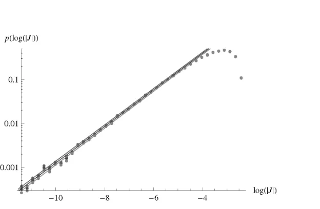
[image:21.595.166.478.462.666.2]Punif(|J| ≤10−4)≈7%. (93)
Figure 1: Probability distribution for log|J|using theSU(3)-invariant flag measure, with fit top(|J|)∝ |J|λ
.
measure induced by aSU(3)-invariant flag metric or the Kaluza-Klein metric, maybe contrary to
what one might expect. Values ofJ close to its maximal value of 1
6√3 ≈0.0962 are disfavored in
[image:22.595.163.440.130.296.2]both cases. Therefore we have used a logarithmic scale for|J|.
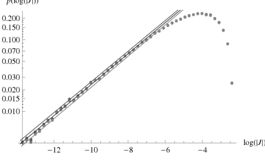
Figure 2: Probability distribution for log|J|using the Kaluza-Klein measure, with fit top(|J|)∝ |J|λ
.
In all three cases the numerical results for small|J|are well approximated by a power law of the form
p(|J|) =α· |J|λ for the probability density of|J|. The logarithmic graphs showp(log|J|)∝ |J|λ+1.
For theSU(3)-invariant flag measure (Fig. 1), the best fit to the data in the region below|J|= 10−2.3
or log|J|=−5.3 is
λflag=−0.042(±0.006), αflag= 18.1(±0.7) ; (94)
for the Kaluza-Klein measure (Fig. 2) we fitted the data in the region below |J| = 10−2.7 or
log|J|=−6.2 and obtained
λKK=−0.097(±0.008), αKK= 18.9(±1.0) ; (95)
finally for the uniform measure (Fig. 3), the best fit to the data in the region below |J|= 10−3.4
Figure 3: Probability distribution for log|J|using a uniform distribution, with fit top(|J|)∝ |J|λ
[image:22.595.164.435.525.690.2]or log|J|=−7.8 is
λunif =−0.500(±0.005), αunif = 3.51(±0.15). (96)
4.2
Wolfenstein parametrization
A different parametrization of the Kobayashi-Maskawa matrix which is frequently used was
intro-duced by Wolfenstein and is based on the experimentally observed hierarchy
y≪x≪z≪1 (97)
in the mixing angles. One rewrites [18]
sinz=λ , sinx=Aλ2, sinye−iw=Aλ3(ρ−iη) (98)
and treatsλas a small parameter whileA, ρ, andηare supposed to be parameters of order unity. In
the modern literature one also frequently uses ¯ρ,η¯instead ofρandηbecause then the combination ¯ρ+
iη¯is independent of the phase convention in the Kobayashi-Maskawa matrix [19]. These parameters
are defined by
ρ=
r
1−A2λ4
1−λ2
¯
ρ−A2λ4(¯ρ2+ ¯η2)
(1−A2λ4ρ¯)2+A4λ8η¯2, η= r
1−A2λ4
1−λ2
¯
η
(1−A2λ4ρ¯)2+A4λ8η¯2. (99)
The experimental values forλ, A,ρ,¯ η¯are [19]3
λ= 0.2272±0.0010, A= 0.818+0.007−0.017, ρ¯= 0.221+0.064−0.028, η¯= 0.340+0.017−0.045. (100)
One viewpoint on the Wolfenstein parametrization is that it is adapted to the values for the
Kobayashi-Maskawa matrix entries that we observe and has no deeper significance; but often the
viewpoint is expressed that this parametrization expresses some kind of “natural hierarchy” in the
mixing angles coming from physics beyond the standard model (see e.g. [20]). Treating the other
parameters as “naturally of order unity” reduces our calculations to a one-dimensional problem as
everything is only expanded in terms ofλ. We find that the SU(3)-invariant measure on the flag
manifold is now, to leading order inλ,
∂(x, y, z, w)
∂(λ, A,ρ,¯ η¯)
√g
∝A3λ11 1 +λ2+O(λ4)
, (101)
and the Jarlskog invariantJ is
J =A
2ηλ¯ 6(1−A2λ4) 1−λ2−2A2ρλ¯ 4−A2(¯η2+ (¯ρ−2)¯ρ)λ6+A4(¯η2+ ¯ρ2)λ8
(1−λ2) (1−2A2ρλ¯ 4+A4(¯η2+ ¯ρ2)λ8)2 =A
2ηλ¯ 6+O(λ10).
(102)
Inverting this expression to leading order gives the probability distribution forJ
p(J)∝ AJη¯2 1 +
J
A2η¯
1/3
+O(J2/3)
!
, (103)
3
Note that only even powers ofλappear in all expansions, so that it isλ2
which is incompatible with the numerical results. Trying to improve this approximate result by
lettingA,ρ¯and ¯η take all possible values leads to inconsistencies since the expansion in powers ofJ
contains poles of arbitrary order inA. From our present viewpoint, where no mechanism for fixing
these parameters close to one is known, the Wolfenstein parametrization seems rather misleading
when discussing geometric probability.
5
Quark Mass Matrices and Gaussian Weighting Functions
In the previous sections we have focussed onU(1)2\SU(3)/U(1)2, the space of Kobayashi-Maskawa
matrices, as the space of CP violating parameters. Since SU(3) is compact, this space has finite
volume for a natural measure. But the Kobayashi-Maskawa matrix is derived from the Hermitian
quark mass matrices, which could be viewed as more fundamental and more directly determined
by physics beyond the standard model. In this section, we try to obtain statistics of the Jarlskog
invariantJ from a random distribution on the space of 3×3 Hermitian matrices.
5.1
Distributions on Hermitian matrices
We follow Sec. 1.2 and write the quark mass matrices as
U mU† = diag(mu, mc, mt), U′m′U′†= diag(md, ms, mb). (104)
whereU andU′ should be thought of as elements ofU(1)2\SU(3). Following [12] we normalize the
mass matrices by dividing by mass scales Λ and Λ′ (often taken to be the top and bottom quark
mass, respectively) which may be chosen for convenience:
M =U†DU , M′ =U′†D′U′. (105)
The matrices D and D′ are now dimensionless quantities, and it is clear that U and U′ are only
defined up to left multiplication by elements of U(1)2. We consider Λ and Λ′ as arbitrary mass
scales, and so we will allow arbitrary eigenvalues for both matrices, instead of fixing one of them to
be one.
A natural measure on the space of Hermitian matrices is induced by the metric
ds2= Tr(dM·dM) = Tr (dD·dD) + 2Tr dU U†D2
− dU U†2
D2 (106)
which is invariant under conjugation underU(3). If we define right-invariant one-formsτa by
dU U† = iλaτa, (107)
this becomes4[withD≡diag(D
1, D2, D3)]
ds2 = Tr (dD·dD)−2τaτbTr (λa[D, λb]D)
= dD21+dD22+dD32+ 2
(D1−D2)2(τ12+τ22) + (D1−D3)2(τ42+τ52)
+(D2−D3)2(τ62+τ72) . (108)
4
The corresponding volume form is
(D1−D2)2(D1−D3)2(D2−D3)2dD1∧dD2∧dD3∧τ1∧τ2∧τ4∧τ5∧τ6∧τ7. (109)
As explained above, the measure on the coset U(1)2\SU(3) is unique and equal to the measure
induced from the bi-invariant metric onSU(3). We obtain a Riemannian measure
DM := (D1−D2)2(D1−D3)2(D2−D3)2sin 2xcos3y siny sin 2z dD1dD2dD3dx dy dz dw dr dt
(110)
on the space of Hermitian 3×3 matrices. The coordinates (x, y, z, w, r, t) on U(1)2\SU(3) were
introduced in Sec. 2, and we allow arbitrary eigenvalues. (In a fermionic mass term, the sign of the
mass has no physical significance, since it can be reversed by multiplying the spinor fields byγ5;
onlym2enters in physical quantities.)
From the expressions (105), it is apparent that each Hermitian matrix with three distinct
eigen-values is associated with six different elements ofR3×U(1)2\SU(3), related by the action of the
discrete groupS3:
M =U†DU = (U†P−1)P DP−1(P U) =: ˜U†D˜U ,˜ P ∈S3, (111)
whereS3 is the symmetric group of degree 3 (the dihedral group of order 6, sometimes denoted by
D3 or D6) which permutes the canonical basis vectors ofR3. The set of matrices with coinciding
eigenvalues has zero measure and hence can be ignored in the present discussion.
Thus we need to consider the spaceR3×(U(1)2×S
3)\SU(3) instead, restricting the coordinates
on the flag manifold to an appropriate range to pick one of the six matrices related by theS3action.
We can use the fact that theS3 action permutes the rows of anSU(3) matrix to demand that the
elements of the third column (see Sec. 2) satisfy the relation
|siny| ≤ |sinxcosy| ≤ |cosxcosy|, (112)
which restricts the coordinatesxandy to
0≤y≤arctan(sinx), 0≤x≤ π4. (113)
Using the natural measure on the flag manifold, we see that this region has precisely one-sixth
of the total volume of the flag manifold:
π/2 R 0
dz
π/4 R 0
dx
arctan(sinx) R 0
dy sin 2xcos3y siny sin 2z
π/2 R
0
dz
π/2 R
0
dx
π/2 R
0
dy sin 2xcos3y sinysin 2z
= 1
6. (114)
An integral overR3with the given measure diverges. We could introduce a cutoff for the quark
masses, but then any expectation values for quark masses would strongly contradict observation, as
We therefore choose to introduce a weighting function in the measure which decays sufficiently
fast for large positive or negative eigenvalues and is able to reproduce the known hierarchy. The
simplest assumption is to take a weighting function of the form
f Tr(M2A)
f Tr((M′)2A′)
, (115)
where A and A′ are Hermitian and positive definite, and we shall further assume [A, A′] = 0.
By a redefinition of M and M′ by unitary conjugation by the same unitary matrix, which leaves
J invariant, one can simultaneously diagonalize A and A′. For simplicity and ease of technical
calculations, we shall choose the functionf in (115) to be a decaying exponential soM andM′ are
governed by Gaussian distributions. Our proposal is to fit the diagonal matricesA and A′ to the
observed quark masses and use the resulting probability distribution for statistics ofJ.
An integral of a quantity such asJ2 becomes5
hJ2i = N
Z
DM DM′e−Tr(M2A)−Tr((M′)2A′)J2(M, M′) (116)
= N
Z
R6
dD dD′
Z
((U(1)2
×S3)\SU(3))2
DU DU′e−Tr(D2
UAU†)
−Tr((D′)2
U′A′U′ †)
J2(U, U′).
Here DU and DU′ are the measures on (U(1)2×S
3)\SU(3) and dD := (D1 −D2)2(D1−
D3)2(D2−D3)2dD1dD2dD3etc., and the normalization factorN is defined by
1
N :=
Z
R6
dD dD′
Z
((U(1)2
×S3)\SU(3))2
DU DU′e−Tr(D2UAU†)−Tr((D′)2U′A′U′ †). (117)
FromJ =Im V11V22V12∗ V21∗andV =U U′†, we have
J(U, U′) =
3 X
a,b,c,d=1
Im U1aU2bU1c∗U2d∗ U′∗1aU′∗2bU′2cU′1d. (118)
At this point, it is perhaps instructive to note that setting A equal to the identity would split
the integral (116) into a product of an integral over the eigenvalues which just gives a constant and
an integral ofJ2 over ((U(1)2×S
3)\SU(3))2. Since all even powers of J are invariant under the
S3 action on U and U′, this can be replaced by an integral over (U(1)2\SU(3))2 if averages are
concerned. By the arguments presented in Sec. 3.1, a change of coordinates reduces this to a single
integration over a flag manifold, and one recovers the results of Sec. 3.1 for expectation values of
powers ofJ.
The introduction of more general diagonal matrices Aand A′ means that the invariance of the
measureDM DM′under separate conjugation ofMandM′by arbitrary elements ofU(3),i.e.under
the action of U(3)×U(3), is broken down to the action of the diagonal subgroup U(1)2×U(1)2
which commutes with A and A′. We find that this symmetry breaking is necessary to obtain a
distribution that reproduces different expectation values for squared quark masses.
It should be clear from (116) that multiplying A (orA′) by a constant is the same as rescaling
the eigenvaluesDi (or Di′) and so amounts to a rescaling of Λ (or Λ′). We can therefore, without
5
any loss of generality, choose A=
1 0 0
0 1/µ2
c 0
0 0 1/µ2
u
, A′=
1 0 0
0 1/µ2
s 0
0 0 1/µ2
d , (119)
whereµc, µu, µs, andµd are dimensionless parameters that we are free to choose so as to reproduce
the observed quark masses as expectation values. (In the case of an exponential exp(−Tr(D2A)),
these would of course be equal to the respective quark masses, expressed in units where Λ =mtand
Λ′ =m
b.) Because of experimental uncertainties in the up and quark masses, one can modify this
distribution to reproduce different values for these masses.
It seems practically impossible to evaluate the integral (116), as the expression forJ in terms of
coordinates on ((U(1)2×S
3)\SU(3))2is too complicated to be given explicitly. However, since
Tr(D2U AU†) =X
a
D2a
X
c
Ac|Uac|2=:
X
a
Da2ξa, Tr((D′)2U′A′U′†) =:
X
a
(Da′)2ξa′ (120)
with
ξ1=A1cos2ycos2z+A2cos2ysin2z+A3sin2y , ξ1′ =A′1cos2y′cos2z′+A′2cos2y′sin2z′+A′3sin2y′,
(121)
and we assumeA3≫1 andA′3≫1, the integrand is negligibly small unlessy≈0 andy′≈0. We
use this to approximate the integrals overyandy′:
arctan(sinx) Z
0
dy
arctan(sinx′)
Z
0
dy′ cos3y siny cos3y′ siny′e−Tr(D2
UAU†)
−Tr((D′)2
U′A′U′ †)
J2(U, U′)
≈
arctan(sinx) Z
0
dy
arctan(sinx′)
Z
0
dy′y y′e−A3y
2 −A′
3(y
′)2
e−Tr(D2UAU†)−Tr((D′)2U′A′U′ †)J2(U, U′) y=y′=0
≈ 4A1
3A′3
e−Tr(D2UAU†)−Tr((D′)2U′A′U′ †)J2(U, U′)
y=y′=0. (122)
It turns out that this is independent ofwandw′. Constant prefactors such as 1/4A3A′
3appearing
in both numerator and denominator can be dropped, and so we have
hJ2i ≈
R
R6dD dD′
R
d4xR
d4x′ sin 2xsin 2zsin 2x′sin 2z′e−Tr(D2UAU†)−Tr((D′)2U′A′U′ †)J2(U, U′) y=y′=0
R
R6dD dD′
R
d4xR
d4x′ sin 2xsin 2zsin 2x′sin 2z′ e−Tr(D2UAU†)−Tr((D′)2U′A′U′ †)
y=y′=0
,
(123)
where
Z
d4x≡
π/4 Z 0 dx π/2 Z 0 dz 2π Z 0 dr 2π Z 0 dt (124)
and similarly forR