This is a repository copy of
Robust optimality of linear saturated control in uncertain linear
network flows.
.
White Rose Research Online URL for this paper:
http://eprints.whiterose.ac.uk/89755/
Version: Accepted Version
Proceedings Paper:
Bagagiolo, F. and Bauso, D. (2008) Robust optimality of linear saturated control in
uncertain linear network flows. In: 47th IEEE Conference on Decision and Control, 2008.
CDC 2008. 47th IEEE Conference on Decision and Control, 9-11 Dec, 2008, Cancun,
Mexico. IEEE , 3676 - 3681. ISBN 978-1-4244-3123-6
https://doi.org/10.1109/CDC.2008.4738842
[email protected] https://eprints.whiterose.ac.uk/ Reuse
Unless indicated otherwise, fulltext items are protected by copyright with all rights reserved. The copyright exception in section 29 of the Copyright, Designs and Patents Act 1988 allows the making of a single copy solely for the purpose of non-commercial research or private study within the limits of fair dealing. The publisher or other rights-holder may allow further reproduction and re-use of this version - refer to the White Rose Research Online record for this item. Where records identify the publisher as the copyright holder, users can verify any specific terms of use on the publisher’s website.
Takedown
If you consider content in White Rose Research Online to be in breach of UK law, please notify us by
Robust optimality of linear saturated control in uncertain linear
network flows
Fabio Bagagiolo and Dario Bauso
Abstract— We propose a novel approach that, given a linear
saturated feedback control policy, asks for the objective func-tion that makes robust optimal such a policy. The approach is specialized to a linear network flow system with unknown but bounded demand and politopic bounds on controlled flows. All results are derived via the Hamilton-Jacobi-Isaacs and viscosity theory.
Keywords: Optimal control, Robust optimization, Inventory control, Viscosity solutions.
I. INTRODUCTION
Consider the problem of driving a continuous time state
z(t) ∈ IRm within a target set T = {ξ ∈ IRm : |ξ| ≤
ǫ} in a finite time T ≥ 0 with ǫ ≥ 0 a-priori chosen
and keeping the state within T from time T on. Such a
problem is shortly referred to as theǫ-stabilizability problem
of z(t). Define u(t) ∈ IRm the controlled flow vector,
w(t) ∈ IRn an Unknown But Bounded (UBB) exogenous
input (disturbance/demand) withn < m, and letD∈Rn×m
a given matrix, U = {µ ∈ IRm : u− ≤ µ ≤ u+} and
W ={η ∈Rn : w− ≤η ≤w+} be two hyper-boxes with
assigned u+,u−,w+ andw−. Also, letσ be a binary state
such that σ(t) = 0if z(t) 6∈ T andσ(t) = 1if z(t)∈ T. The robust counterpart of the problem takes on the form
min
u∈Uwmax∈W J(ζ, u(.), w(.)) =
Z ∞
0
e−λ(σ)tgσ(z(t), u(t))dt (1)
˙
z(t) =u(t)−Dw(t), z(0) =ζ for allt≥0 (2)
z(t)∈ T for allt≥T , (3)
where we denote by U = {u : [0,+∞[→ U} and by
W ={w : [0,+∞[→ W} the sets of measurable controls
and demands respectively. From a game theoretic standpoint
we will consider two players, player 1 playinguand player
2 playingw. The statez(t)has initial valueζand integrates the discrepancy between the controlled flowu(t)andDw(t)
as described in (2). Controls u(t) and demand w(t) are
bounded within hyperboxes by their definitions. Condition
(3) guarantees the reachability of the target set from timeT
on. Among all controls satisfying the above conditions (call it admissible controls or solution), we wish to find the one that minimizes the objective function (1) under the worst demand. The objective function is defined on an infinite horizon with discount factore−λ(σ)tdepending onσ. The reason for such
a dependency on σ will be clearer later on. The integrand
This work was not supported by any organization
F. Bagagiolo is with Dipartimento di Matematica, Universit`a di Trento, Via Sommarive, 14, 38050 Povo di Trento (TN), Italy,
D. Bauso is with DINFO, Universit`a di Palermo, 90128 Palermo, Italy,
in (1) is a function ofz anduand its structure depends on
σas follows
gσ(z(t), u(t)) =
½
˜
g(z(t), u(t)) if σ= 0(z(t)6∈ T)
ˆ
g(z(t), u(t)) if σ= 1(z(t)∈ T) (4) where˜g(.)andgˆ(.)have to be designed as explained below. In a previous work [2], it has been shown that under certain
conditions on the matrix D (recalled below), the following
(linear) saturated control policy drives the statez withinT:
u(t) =sat[u−,u+](−kz(t)) :=
:=¡
sat[u−,u+](−kz1(t)), ..., sat[u−,u+](−kzn(t))¢∈IRn,
(5) withk >0and where
sat[α,β](ξi) =
β, if ξi> β,
ξi, if α≤ξi≤β,
α, if ξi < α.
Then, we deduce that the saturated control policy returns an admissible solution for problem (1)-(3). In the light of this consideration, we focus on the following problem.
Problem 1: We wish to design the integrandgσ(.)of the
objective function (1) in (4) such that the saturated control turns optimal for the min-max problem (1)-(3).
A. Literature and main results
In this work, we add new results concerning the optimality of the saturated control policy, which is proved to solve the
ǫ-stabilizability problem in [2]. Our interest for the saturated control is also due to the fact that it represents the simplest form of a piece-wise linear control [6]. The idea of modeling the demand as unknown but bounded variable is in line with some recent literature on robust optimization [3], [5], [10] though the “unknown but bounded” approach has a long history in control [4]. The conservative approach of Section V reminds the Soyster decomposition [12], used in robust linear programming. Also, the notion of feedback in control, present in this work, reminds the notion of
recourse used in robust optimization [7]. Concerning the
B. Some basic facts about Hamilton-Jacobi equations, opti-mal control and differential games
A Hamilton-Jacobi equation is a first order partial differ-ential equation of the form
F(x, v(x),∇v(x)) = 0 inΩ,
where Ω ⊆ IRm, is open, F : Ω×IR×IRm → IR is
continuous. A viscosity solution of it is a continuous function
v : Ω → IR such that, for every x ∈ Ω and for every
differentiable functionϕ: Ω→IR, the following holds
i) xis local max forv−ϕ ⇒ F(x, v(x),∇ϕ(x))≤0;
ii) xis local min for v−ϕ ⇒ F(x, v(x),∇ϕ(x))≥0.
The idea is hence to substitute the derivatives ofv, which
usually do not exist, with the derivatives of the test function
ϕ, and to require that the equation is ”semi-verified” in
the point of maximum for v −ϕ and (oppositely)
”semi-verified” in the point of minimum for v−ϕ. If a function
satisfies i) only (for every test functions) then it is called a subsolution, whereas it is called a supersolution in the other case. Such a notion of solution goes back to Crandall-Evans-Lions [8]. Obviously, this is a weak definition of solution, and in particular, if a functionvis a classical solution (i.e. it is differentiable and satisfies the equation by equality), then it is also a viscosity solution.
Let us consider an optimal control problem
max
β J(x, β)
µ
= max
β
Z ∞
0
e−tℓ(y(t), β(t))dt
¶ ,
subject to y˙(t) =f(y(t), β(t)), y(0) =x,
where β : [0,+∞[→B is the measurable control, with B
a compact set. Under rather general hypotheses, the value function of the problem,U(x) = supβJ(x, β), is a viscosity
solution of the Hamilton-Jacobi-Bellman equation
U(x) + min
b∈B{−f(x, b)· ∇U(x)−ℓ(x, b)}= 0.
Such an equation holds in the whole IRm if the control
problem is without state-constraints (i.e. the statey(·)is free
to move inIRm); otherwise, if the problem is confined in the
closure Ω of an open set Ω, the equation must be coupled
with suitable boundary conditions on ∂Ω, usually given by
an exit costψ fromΩ. The problem is then
max
β J(x, β)
³
= maxβR tx(β)
0 e
−tℓ(y(t), β(t))dt+
+e−tx(β)ψ(y(t))¢ ,
wheretx(β) is the first exit time from Ω for the trajectory
starting fromxwith controlβ (with the conventiontx(β) =
+∞if the trajectory never exit fromΩ).
Under some hypotheses on the regularity of ∂Ω and
on the existence of inner suitable fields on the points of the boundary, the value function turns out to satisfy the
boundary condition U = ψ in the so-called ”viscosity
sense”. This means that on the point x of the boundary
which are of local maximum (respectively local minimum)
for U −ϕ (when restricted to the closure of Ω), we must
have U(x) ≤ ψ(x) (resp. U(x) ≥ ψ(x)) or U(x) +
minb∈B{−f(x, b)· ∇ϕ(x)−ℓ(x, b)} ≤ 0 (resp. ≥0), i.e.
the equation holds with the ”right” sign.
Under general hypotheses (on the regularity of Ω, and
some ”compatibility conditions” for the exit-cost ψ), the
value function is characterized as the unique bounded uni-formly continuous viscosity solution of the boundary value problem for the Hamilton-Jacobi-Bellman equation (note that
ifΩisIRm, then there are not boundary conditions).
Now we consider a differential game with state equation
y′(t) =f(y(t), α(t), β(t)), y(0) =x,
and cost functional
J(x, α, β) =
Z +∞
0
e−tℓ(y(t), α(t), β(t))dt,
for the infinite horizon case (i.e. without restriction toΩ), or
J(x, α, β) = Rtx(α,β)
0 e
−tℓ(y(t), α(t), β(t))dt+
+ e−tx(α,β)ψ(y(t)), (6)
for the exit-time problem. The measurable controlα∈ A=
{α : [0,+∞[→ A, measurable} is governed by the first
player who wants to minimize the cost, whereas and the
second player, by choosing the measurable controlβ ∈ B=
{β : [0,+∞[→ B, measurable}, wants to maximize the
cost. We define the non-anticipative strategies (see, e.g., [9]) for the first player
Γ =nγ:B → A, β7→γ[β]¯¯
¯β1=β2 in[0, s] =⇒ γ[β1] =γ[β2]in[0, s]}.
(7)
Hence the (lower) value function for the minimiza-tion/maximization problem is defined as
V(x) = min
γ∈Γmaxβ∈BJ(x, γ[β], β).
Under rather general hypothesis, the value functionV is the
unique bounded uniformly continuous viscosity solution of the following Hamilton-Jacobi-Isaacs equation
V(x) + min
b∈Bmaxa∈A{−f(x, a, b)· ∇V(x)−ℓ(x, a, b)}= 0,
which also in this case must be coupled with appropriate boundary conditions for the exit-time problem.
II. SOLUTION APPROACH
We will pursue the idea of decomposing the infinite
horizon (1) into a finite horizon problem with σ(t) = 0
and an infinite infinite horizon problem with σ(t) = 1 as
expressed below
J(ζ, u(.), w(.)) = [RT
0 g˜(z(t), u(t), w(t))dt+
R∞
T e
−tˆg(z(t), u(t), w(t))dt]. (8)
We can do such a decomposition as once the state enters the
targetT it will remain in it for the rest of the time [2].
Let us now explain more in details the notion of optimality
of a saturated control mentioned in Problem 1. Let U and
Introduction (after equation (3)), and letΓbe the set of
non-anticipative strategies for the player 1 (see (7), replacing B
byW,AbyU, andβ byu). The (lower) value function for
the differential game is then
V(ζ) = inf
γ∈Γwsup∈WJ(ζ, γ[w], w),
whereζis the initial state. Now,V must be the unique
vis-cosity solution of the Hamilton-Jacobi-Isaacs (HJI) equation
σV(ζ) +H(ζ,∇V(ζ)) = 0, (9)
where the HamiltonianH is, for every(ζ, p)∈IRm×IRm:
H(ζ, p) := min
ω∈Wmaxµ∈U{−(µ−Dω)·p−g
σ(ζ, µ, ω)}. (10)
Observe that the above equation depends on functiongσ(.)
and onσ. Hence when dealing with the infinite horizonσ=
1 and so in the left hand side of the equation there is the
presence of the addend+V(ζ). We can look at the saturated
control as a special non anticipative strategyγ0, namely, for
everyw∈W we define
γ0[w](t) =sat[u−,u+](−kz),
where z is the state trajectory of (2) under the saturated
control as choice for u and under the choice of w. Given
this, we wish to find a functiongσ(.)such that the worst cost
returned by the saturated control equals the value function
V. This corresponds to imposing
˜
V(ζ) := sup
w∈W
J(ζ, γ0[w], w) =V(ζ),
i.e. we get the robust optimality of the saturated control if
˜
V =V, (11)
whereV˜ is obtained by maximizing overw
˜
J(ζ, w) =
Z T
0
e−σ(t)tgσ(z(t), sat[u−,u+](−kz(t)), w(t))dt,
(in the infinite horizon the extremes are T and ∞) subject
to the controlled dynamics
˙
z(t) =sat[u−,u+](−kz(t))−Dw(t), z(0) =ζ (orz(T) =ζ).
Now, V˜ must be the unique viscosity solution of the
Hamilton-Jacobi-Bellman (HB) equation:
σV˜(ζ) + ˜H(ζ,∇V˜(ζ)) = 0, (12)
where the HamiltonianH˜ is, for every(ζ, p)∈IRm×IRm
˜
H(ζ, p) := minω∈W{−(sat[u−,u+](−kζ)−Dω)·p+
−gσ(ζ, sat
[u−,u+](−kζ), ω)}.
In the following, we will look for suitable cost g in
order to get the optimality of the saturated control for the corresponding problems. We will prove such an optimality (i.e. (11)) in two different ways: i) directly computing the
functions V, V˜ and checking their equality, 2) writing the
two corresponding Hamilton-Jacobi equations and checking they have the same unique solution.
Remark 1: A trivial choice isgσ(ζ, µ, ω) =|sat(−kζ)−
µ|. It penalizes any control u different from the saturated
control. However, such a choice makes the game (and the mathematical problem) without interest.
III. MINIMUM TIME PROBLEM OUTSIDE THE TARGET SET
Let us start by observing that we can always choose˜g(.)
big enough in comparison withˆg(.)such that, for all uand
w, the second contribution RT∞gˆ(z(t), u(t), w(t))dt in (1) can be neglected if compared with the first contribution
RT
0 ˜g(z(t), u(t), w(t))dt. In particular this is true if we
chooseg˜(ζ, µ, ω) = M withM > 0 big enough. With the
above choice the problem outside the targetT is equivalent
to a minimum time problem with˜g(ζ, µ, ω)≡1. With this in
mind, take without loss of generalityU ={µ∈IRm¯¯
¯−1≤ µi≤1 ∀i= 1, .., m},W ={ω∈IRn
¯ ¯
¯−1≤ωj ≤1 ∀j=
1, ..., n}, and D an m×n matrix satisfying U ⊃ DW.
We denote by Dij the entries of the matrix. The target
is T = {ξ ∈ IRm¯¯
¯|ξi| ≤ (1/k) ∀i = 1, ..., m}, and the
saturated control policy isu(t) =sat[−1,1](−kz(t)). Hence,
the two Hamiltonians become, for allζ, p∈IRm(recall that
we are considering˜g≡1),
H(ζ, p) =−
n
X
j=1
¯ ¯ ¯ ¯ ¯
m
X
i=1 piDij
¯ ¯ ¯ ¯ ¯
+
m
X
i=1
|pi| −1,
˜
H(ζ, p) =−
n
X
j=1
¯ ¯ ¯ ¯ ¯
m
X
i=1 piDij
¯ ¯ ¯ ¯ ¯
−
m
X
i=1
sat[−1,1](−kζi)pi−1
(13)
By our hypotheses, the controllable set is IRn\ T, and
henceV andV˜ are, respectively, the unique solutions of
½
H(ζ,∇V(ζ)) = 0 inIRn\ T
V = 0 on ∂T;
½ ˜
H(ζ,∇V˜(ζ)) = 0 inIRn\ T
˜
V = 0 on ∂T;
(14)
The question is then to prove that such two problems have
the same solution (note that we do not a priori knowV and
˜
V). Anyway, in this case, due to the structure of the system
and to other hypotheses, we can easy guess that the saturated control is an optimal choice for player 1. Indeed, since, whateverw(t)is, for everyi-th component,(Dw(t))icannot
change the sign ofsat[−1,1](−kzi(t))−(Dw(t))i (when the
initial point satisfies|ζi|>(1/k)), and since that is the “good
sign” for steeringζto the target, then any controller will use such a control (or non anticipative strategy).
In the light of the above considerations, for the value function, it is reasonable to consider the following expression
V(ζ) = max
i=1,...,m
(
max©
0,|ζi| −1k
ª
1−Pn
j=1|Dij|
)
. (15)
That isV is the time requested for steering all the
compo-nents in the interval [−1/k,1/k], under the worst scenario
concerning the demandw.
Leti∗be the solution of the above maximization (the last
component to reach the target set), the generic component of the costate is pi∗ = 1−Pn1
j=1|Di∗j| and pj = 0 for all
j 6= i∗. The optimal choice for w is w
differentiable. On the other hand, on the points where it is not differentiable (i.e. the point where the maximizing index in (15) changes), the definition of viscosity solution applies. We can also note that, on such points of non-differentiability (which are located on some portion of hyperplanes), we can
only have test functionϕ such thatV −ϕhas a minimum,
and also that thei-th component of the gradient∇ϕhas the
same sign ofζi. Hence the left-hand side of the equations in
(14) are the same (see also (13)).
It must be noted that while the saturated control is unique
optimal for the component i∗, this is no longer true for all
the other components j 6= i∗. Actually, all z
j with j 6=i∗
once reached the target may exit and enter again several times following an infinite number of different trajectories and this until alsozi∗ reaches the target set.
IV. A “QUADRATIC COST”WITHIN THE TARGET SET
Within the target set we consider the following quadratic cost depending onζ, µ, ω for fixed k >0:
ˆ
g(ζ, µ, ω) = k+ 1 2 kζ+
Dω k k
2+1
2kkµ−Dωk
2+CkD(ω−ω¯)k2,
where, k · k is the euclidean norm in IRn, ω ∈ W is a
generic vertex, a-priori chosen, ofWandC≥0is a suitable
constant, which will be fixed later. Our guess is that, inside
the target T, the saturated control is the unique optimal
strategy for the min-max problem related to the cost gˆ(.),
and suitable exit-cost from the closed setT.
Since we are decoupling the initial problem in two
prob-lems, outside and inside the targetT, in this section we may
consider the infinite horizon problem with initial timeT = 0.
First of all, let us consider the maximization problem over
w∈W, with controluequal to the linear saturated one:
˜
V(ζ) = sup
w∈w
Z ∞
0
e−tgˆ(z(t),−kz(t), ω),
subject toz˙(t) =−kz(t)−Dω, z(0) =ζ∈ T.
(16)
Note that here we are not imposing an exit cost from T.
Indeed, it is without meaning in this case since, whichever
the controlwis, the trajectory can not exit fromT.
We now specialize the constantC≥0in the definition of
the costgˆ. We choose a vertexωofW, andC≥0such that,
for allζ∈ T, the maximum overω∈ W of the expression
2k+ 1 2
° ° ° °
ζ+Dω k
° ° ° °
2
−ζ·Dω
k +
Dω k ·
Dω
k +CkD(ω−ω¯)k 2,
(17)
is always taken in−ω (note that the first addendum of such
expression is just the sum of the two first addenda ofgwhen
µ=−kζ). This is possible by choosing ω equal to one of
the two opposite vertices which strictly maximize the norm
ofDω(which exist since we may suppose the matrixDhave
positive entries), and then takingC such that
C≥maxζ∈T,ω∈vertW,ω6=−ω
2k+1
k
³ kζ+Dω
k k
2
−kζ−Dω
2 k 2´
+ 4kDωk2−kDω−Dωk2
−ζ·(Dω+Dω)+Dω·(Dω+Dω)
k2 .
(18)
Now, if we fix w(t) ≡ −ω for all t, then, since u(t) =
−kz(t), the trajectory is given by
z(t) =e−kt
µ ζ−Dω
k 
+Dω k .
Hence, the cost associated to such a choice of w is (after
simple calculation)
˜ J(ζ) =1
2
° ° ° °
ζ−Dω
k ° ° ° °
2
+ 4CkDωk2,
We guess, not surprisingly, that J˜ is indeed the value
functionV˜ of the maximization problem. This can be done,
for instance, by proving that J˜ solves the corresponding
Hamilton-Jacobi equation
˜
J(ζ)+ min
ω∈W n
−(−kζ−Dω)· ∇J˜ω(ζ)−ˆg(ζ,−kζ, ω)
o
= 0.
(19)
This can be easily checked, since J˜ is differentiable and
hence a classical solution of (19) (when we put the gradient
of J˜inside the equation, by the hypothesis about the
max-imization of (17) we immediately get that the minimum in
the left-hand side is reached in−ω, and hence we conclude).
By uniqueness of the solution of (19),J˜must coincide with
the value functionV˜.
We now consider the differential game, subject to (2), with
running costˆg, and exit-cost from T given by
ψ(ζ) = 1 2kζ−
Dω k k
2+ 4CkDωk2,
Following the solution approach explained in Section II,
we guess that the (lower) value function V for such a
problem, coincides with the functionV˜ = ˜J already found.
By the general results, as explained in the Introduction,
the lower value functionV is the unique bounded continuous
viscosity solution of the boundary value problem
V(ζ) + min
ω∈Wmaxµ∈U {−(µ−Dω)· ∇V(ζ)+ −ˆg(ζ, µ, ω)}= 0 inT, V =ψon∂T,
(20)
where the boundary condition are in the viscosity sense.
If now we specialize a little bit more the constantC≥0
in the definition ofgˆ, we may get thatV˜ is also a solution of (20) (note that it satisfies the boundary condition in the classical way, and hence also in the viscosity sense). This is
possible by the following observations. Let us putV˜ (which
is differentiable) and its gradient in (20). For everyω∈ W,
letµω ∈ U reach the maximum in the left-hand side. Now,
note that our condition onC is only a lower bound. Hence
we may take C larger than its lower bound. In particular,
since, for every ζ ∈ T, µ ∈ U, ω ∈ W, the difference
|ˆg(ζ,−kζ, ω)−ˆg(ζ, µ, ω)|, which is
1 2k
¯ ¯
¯kkζ+Dωk
2
is small of order 1/k, we can takeC a little bit larger than its lower bound such that it is also true that, for everyζ∈ T,
the minimum with respect toω∈ W of the expression
−(µω−Dω)· ∇V(ζ)−g(ζ, µω, ω),
is taken in−ω. But, as standard calculations show, the only
possibility is µ−ω = −kζ and hence V˜ solves (20). By
uniqueness, we then get V˜ = V, and u(t) = −kz(t) is
the unique possibility for optimality.
Remark 2: Argument of future works is searching a
suit-able running costˆg which leaves the demand free to switch
(at least) between two opposite vertices.
V. ACONSERVATIVE APPROXIMATION
In this section, we propose a conservative approach that allows us to solve the original problem without decomposing it into the finite an infinite horizon problem. Let us split the demandw(t)into mindependent demandsw(i)(t)each one acting on a different component. This corresponds to
consideringmdecoupled one-dimensional dynamics of type
˙
zi(t) =ui(t)− n
X
j=1
Dijwj(i)(t).
In the rest of the section, we focus on the one dimensional
version of our problem and drop the indexiwhere possible.
In the one dimensional context, it is natural to think (and we will prove it in the sequel, for a suitable cost) that the optimal choice for the player 2 is to use
w(t) =−sign(z(t)) arg max
ω | n
X
j=1
Dijωj| ∈[−1,1]n, (21)
where, if z(t) = 0, then w(t) may be any value from
[−1,1]n. Now, consider the following objective function
g(ζ, µ) = max{|sat[−1,1](−kζ)|,|µ|},
and the corresponding infinite horizon game with cost
J(ζ, u(.), w(.)) =
Z ∞
0
e−tg(z(t), u(t))dt,
wheree−t is a given discount term. We want to show that
the saturated strategy, is the optimal one for the first player. Hence, first of all, let us prove the (non surprising) optimality of (21) for the second player in the corresponding maximiz-ing optimal control problem whenu(t) =sat[−1,1](−kz(t)), that is when the cost is just equal to |sat[−1,1](−kz(t))|.
Defining c=Pn
j=1|Dij|, the system is (recall0< c <1)
˙
z(t) =sat[−1,1](−kz(t)) +c(sign(z(t))), z(0) =ζ. (22)
Let us suppose −(1/k) ≤ ζ < 0. Then the trajectory is
(recall that if z(t)∈[−(1/k),0[, then sat[−1,1](−kz(t)) =
−kz(t), andsign(z(t)) =−1)
z(t) =e−kt³ζ+ c
k ´
− c
k ∀t≥0
Note that such a trajectory is always negative and hence it is exactly the solution of the system (22) with the second
member given by−kz(t)−c. Moreover, observe that it is
increasing if ζ < −(c/k) and decreasing if −(c/k)< ζ <
0. Hence, in any case, it converges (for t → +∞) to the
equilibrium−(c/k). Note that such an equilibrium point is
just obtained from(cωζ)/k whenωζ =−1, that is whenωζ
solves the problem ωζ(cζ) = max
ω∈[−1,1]ω(cζ). The cost of such a controlled trajectory is
˜ V(ζ) =
Z ∞
0
e−t(−kz(t))dt=k(c−ζ)
k+ 1
Let us note that V˜ has a continuous derivative in
[−()1/k),0[, given by the negative constant V˜′(ζ) ≡
−k/(k + 1). Moreover we have that V˜(ζ) → kc
k+1, for ζ→0− andV˜(ζ)→ kc+1
k+1, forζ→
−
1k.
If insteadζ≤ −(1/k), then the system has the right hand
side equal to 1−c until z reaches the value −(1/k) and
after, again, equal to −kz−c. Since the reaching time is
τ = −(kζ + 1)/(k−kc), dividing the system in the two
intervals of time [0, τ] (with initial point ζ), and [τ,+∞]
(with initial point−(1/k)), we obtain the trajectory
z(t) =
ζ+ (1−c)t 0≤t≤τ,
e−kt+kτ
µc−1 k
¶ −c
k
Again, such a trajectory is increasing and converges to
−(c/k). The corresponding cost and cost derivative in ]−
∞,−(1/k)[are
˜
V(ζ) =−e−τ(1−c) k
k+ 1 + 1, V˜(ζ)
′=e−τ k
k+ 1.
Note thatV˜ is then continuous and derivable, sinceV˜(ζ)→
kc+1
k+1, for ζ→ −
1
k
−
andV˜(ζ)′ → − k
k+1, forζ→ −
1
k
−
. If insteadζ >0, a similar analysis as before gives
˜
V(ζ) = k
k+1(ζ+c) 0< ζ <(1/k) ˜
V(ζ) =−e−τ(1−c) k
k+ 1 + 1 (1/k)≤ζ,
where τ = (1−kζ)/(k−kc) is the reaching time of the
value1/k. Also in this casec/kis an attracting equilibrium
point. Then, the valueV˜ is continuous and derivable in]−
∞,0[∪]0,+∞[. Moreover, it is continuous in ζ= 0 where
it is equal to kc/(k+ 1) but is not derivable in ζ = 0.
The left limit of derivatives is−k/(k+ 1)whereas the right
limit isk/k+1. Hence, in the view of the viscosity solutions
approach, we can say that there are not test functionsϕsuch
that V˜ −ϕhas a local maximum in ζ= 0, whereas the set
of the derivatives in ζ= 0of all test functions ϕ such that
˜
V −ϕhas a local minimum inζ= 0is exactly the interval
[−k/(k+ 1), k/(k+ 1)].
The function V˜ is the optimal value for the problem of
maximizing, amongw∈W, the following cost
˜
J(ζ, w(.)) =
Z ∞
0
|sat[−1,1](−kz(t))|dt,
subject to the dynamics
˙
if and only if it is a viscosity solution in IRof the problem
˜
V(ζ) + min
ω∈[−1,1] {−(sat[−1,1](−kζ)−cω) ˜V(ζ)
′+
−|sat[−1,1](−kζ)|}= 0
Here we do not have boundary conditions since the problem is not restricted to a subset, but it is treated in the whole
IR. A direct calculation shows thatV˜ is a viscosity solution. Now we guess thatV˜ is also a viscosity solution of the Isaacs equation for the differential game given by the cost
J(ζ, u(.), w(.)) =
Z ∞
0
e−tmax{|sat
[−1,1](−kz(t))|,|u(t)|}dt
subject to the dynamics (2). Hence, we have to prove thatV˜
is a viscosity solution of
˜
V(ζ)+ minω∈[−1,1]maxµ∈[−1,1]{−(µ−cω) ˜V(ζ)′+
−max(|sat[−1,1](−kζ)|,|µ|)}= 0
and hence we will get, by uniqueness, that it is equal to the lower value function of the game.
To this end, we have to split the analysis in the following cases: a) ζ < −(1/k), b) −(1/k) ≤ ζ < 0, c) ζ = 0, d)
0 < ζ ≤1/k, e) ζ > 1/k. A careful analysis of all these cases brings the desired result, and also the fact that the linear saturated control is the unique optimal choice for the first player. In particular, outside the target, the optimal choice for the first player is µ = 1 if ζ < 0 (µ = −1 if ζ > 0) which is exactly the linear saturated control, and corresponds to the optimal choice for a minimum time problem.
VI. NUMERICALILLUSTRATIONS
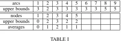
Consider dynamicsx˙ =Bu−wwhereB is the incidence
matrix of the network with n = 5 nodes and m = 9 arcs
in Fig. 1. Table I lists the upper bounds onu(lower bounds
2
3
4
5 1 8
1 2
5
6 4
7
[image:7.612.337.537.53.121.2]9 3
Fig. 1. Example of a system with5nodes and9arcs.
are all 0), the demand bounds, and the long–term average
demands. Now, given the nominal demandw¯ = [0 1 2 1 1]
and the nominal balancing flowu¯= [1 1 1 0 0 1 1 3 2]′∈ U
(which is w¯ = Bu¯) we translate the variables by setting
δu =. u−¯u and δw = w−w¯. We choose matrix D as
in (40) of [2], obtained via constraint generation, (see [2] Section 5.2). We simulate the system under the saturated
linear state feedback control (5) (we initialize x(0) = 0,
y(0) = 0, and set k = 4). The time plot ofz(t) in Fig. 2 shows thatz(t)converges to the interval[−δu+/k,−δu−/k]
(dotted line in Fig. 2).
arcs 1 2 3 4 5 6 7 8 9
upper bounds 3 2 3 3 3 3 3 5 5
nodes 1 2 3 4 5
upper bounds 0 2 3 2 2
averages 0 1 2 1 1
TABLE I
CONTROLLED FLOWS CONSTRAINTS AND DEMAND BOUNDS
0 100 200 300 400 500
−0.5 0 0.5
z1
time
0 100 200 300 400 500
−0.4 −0.2 0 0.2 0.4 0.6
z2
time
0 100 200 300 400 500
−0.5 0 0.5
z3
time
0 100 200 300 400 500
−0.95 −0.275 0.4
z4
time
0 100 200 300 400 500
−0.95 −0.275 0.4
z5
time
0 100 200 300 400 500
−0.5 0 0.5
z6
time
0 100 200 300 400 500
−0.5 0 0.5
z7
time
0 100 200 300 400 500
−0.5 0 0.5 1
z8
time
0 100 200 300 400 500
−0.5 0 0.5
z9
[image:7.612.317.555.155.338.2]time
Fig. 2. The variablez(t)with saturated linear feedback control (5) with k= 4.
REFERENCES
[1] M. Bardi, I. Capuzzo Dolcetta, ”Optimal Control and Viscosity So-lutions of Hamilton-Jacobi-Bellman Equations”, Birkh¨auser, Boston, 1997.
[2] D. Bauso, F. Blanchini, R. Pesenti, “Robust control policies for multi-inventory systems with average flow constraints”, Automatica, 42(8): 1255–1266, 2006.
[3] A. Ben Tal, A. Nemirovsky, “Robust solutions of uncertain linear programs”, Operations Research, 25(1): 1–13, 1998.
[4] D. P. Bertsekas, I. Rhodes, “Recursive state estimation for a set-membership description of uncertainty”, IEEE Trans. on Automatic
Control 16(2): 117–128, 1971.
[5] D. Bertsimas, A. Thiele, “A Robust Optimization Approach to Inventory Theory ”, Operations Research, 54(1): 150–168, 2006.
[6] A. Bemporad, M. Morari, V. Dua, and E. N. Pistikopoulos, “The explicit linear quadratic regulator for constrained systems”, Automatica, 38(1): 3-20, 2002.
[7] X. Chen, M. Sim, P. Sun, and J. Zhang, “A Linear-Decision Based Approximation Approach to Stochastic Programming”, accepted in
Operations Research, 2007.
[8] M.G. Crandall, L.C. Evans, P.L. Lions, “Some properties of viscosity solutions of Hamilton-Jacobi equations”, Trans. Amer. Math. Soc., vol. 282: 487–502, 1984.
[9] R.J. Elliot, N.J. Kalton, “The existence of value in differential games”,
Mem. Amer. Math. Soc., vol. 126, 1972.
[10] O. Kostyukova, and E. Kostina, “Robust optimal feedback for terminal linear-quadratic control problems under disturbances”, Mathematical
Programming, 107(1-2): 131–153, 2006.
[11] H. Michalska, D. Q. Mayne, “Robust Receding Horizon Control of Constrained Nonlinear Systems”, IEEE Trans. on Automatic Control, 38(11): 1623–1633, 1993.
[12] A. L. Soyster, “Convex Programming with Set-Inclusive Constraints and Applications to Inexact Linear Programming”, Operations