This is a repository copy of
Conditional parameter estimates from Mixed Logit models:
distributional assumptions and a free software tool
.
White Rose Research Online URL for this paper:
http://eprints.whiterose.ac.uk/43620/
Article:
Hess, S (2010) Conditional parameter estimates from Mixed Logit models: distributional
assumptions and a free software tool. Journal of Choice Modelling, 3 (2). 134 - 152 . ISSN
1755-5345
Reuse
Unless indicated otherwise, fulltext items are protected by copyright with all rights reserved. The copyright exception in section 29 of the Copyright, Designs and Patents Act 1988 allows the making of a single copy solely for the purpose of non-commercial research or private study within the limits of fair dealing. The publisher or other rights-holder may allow further reproduction and re-use of this version - refer to the White Rose Research Online record for this item. Where records identify the publisher as the copyright holder, users can verify any specific terms of use on the publisher’s website.
Takedown
If you consider content in White Rose Research Online to be in breach of UK law, please notify us by
Conditional parameter estimates from Mixed Logit
models: distributional assumptions and a free software
tool
Stephane Hess∗
July 1, 2010
Abstract
A number of authors have discussed the possible advantages of condition-ing parameter distributions on observed choices when workcondition-ing with Mixed Multinomial Logit models. However, the number of applications is still rel-atively small, partly due to a limited implementation in available software. To address this situation, the present paper discusses the development of a freeware software tool that allows users to compute conditional distributions independently of the software used during model estimation. Additionally, the paper looks at what impact assumptions made for the unconditional distributions have on the results obtained with conditional distributions. Here, an application using stated choice data collected in Denmark shows that while the move from unconditional to conditional distributions possibly brings results closer together, some discrepancies do remain.
KEYWORDS: mixed logit; discrete choice; conditional distributions; taste heterogeneity
1
Introduction
The random coefficients formulation of the Mixed Multinomial Logit (MMNL)
model (cf.Revelt and Train,1998;Train,1998;McFadden and Train,2000;
Hen-sher and Greene,2003;Train,2003) is fast becoming one of the most widely used econometric structures for the analysis of choice behaviour. The main advantage of the MMNL model over its more simplistic closed-form counterparts is that it
∗Institute for Transport Studies, University of Leeds, [email protected], Tel: +44 (0)113
allows for a relaxation of the assumption of constant marginal utility coefficients across individuals.
The MMNL model accommodates taste heterogeneity by allowing marginal utility coefficients to be distributed randomly across respondents. A major issue in this context is the choice of an appropriate mixing distribution in the absence of information on the actual shape of that distribution in the sample population
(see for exampleHensher and Greene 2003,Hess et al. 2005and Fosgerau 2006).
The vast majority of MMNL applications make use of the Normal distribution. Here, problems can arise due to the unbounded nature of the distribution, as well as due to its symmetry assumption. These can lead to issues with sign violations and biased mean values respectively. Indeed, it is in such situations not clear whether the findings actually reflect real sensitivities present in the data or are simply a result of the distributional assumptions. A possible solution is to use more flexible distributions, not making a strict symmetry assumption, while also allowing for the estimation (rather than imposition) of bounds to either side.
Examples of such distributions include the Johnson SB, discussed in detail in a
MMNL context by Train and Sonnier(2005).
A serious problem is that models making use of these more advanced distribu-tions are considerably more difficult to estimate than their counterparts relying on more restrictive distributions, often leading to issues with convergence or pa-rameter significance. Another major issue with the MMNL model is that while it allows the user to accommodate random taste heterogeneity in the sample pop-ulation, it does not directly provide any information on the likely location of a given respondent on this distribution. However, simply knowing that a coefficient varies across respondents is only of limited practical use.
An obvious way of dealing with this second issue is to move from the uncon-ditional (i.e. sample population level) distribution to a conuncon-ditional distribution. This equates to inferring the likely position of each sampled individual on the
distribution of sensitivities (cf. Revelt and Train,1999;Train,2003;Sillano and
Ort´uzar,2004;Greene et al.,2005).
Letβgive a vector of taste coefficients that are jointly distributed according to
f(β|Ω), where Ω is a vector of distributional parameters that is to be estimated
from the data. Let Yn give the sequence of observed choices for respondent
n (which could be a single choice), and let L(Yn|β) give the probability of
observing this sequence of choices with a specific value for the vector β. Then
it can be seen that the probability of observing the specific value ofβ given the
choices of respondentnis equal to:
L(β|Yn) =
L(Yn|β)f(β |Ω)
R
βL(Yn|β)f(β |Ω) dβ
The integral in the denominator of Equation1 does not have a closed form so-lution, such that its value needs to be approximated by simulation. This is a simple (albeit numerically expensive) process, with as an example the mean for
the conditional distribution for respondentn being given by:
c
βn=
PR
r=1[L(Yn|βr)βr]
PR
r=1L(Yn|βr)
, (2)
whereβrwithr= 1, . . . , Rare independent multi-dimensional draws1with equal
weight from f(β|Ω) at the estimated values for Ω. Here, βcn gives the most
likely value for the various marginal utility coefficients, conditional on the choices
observed for respondentn.
It is important to stress that the conditional estimates for each respondent
follow themselves a random distribution, and that the output from Equation 2
simply gives the expected value of this distribution. As such, a distribution of the
output from Equation2 across respondents should not be seen as a conditional
distribution of a taste coefficient across respondents, but rather a distribution of the means of the conditional distributions (or conditional means) across re-spondents. Here, it is similarly possible to produce a measure of the conditional standard deviation, given by:
f
βn=
v u u u t PR r=1
L(Yn|βr)
βr−cβn
2
PR
r=1L(Yn|βr)
, (3)
withβcn taken from Equation2.
Obtaining information on the likely location of a given respondent on the distribution of tastes across the sample population can be a great asset for
var-ious reasons. Here, Greene et al. (2005) and Hess (2007) amongst others show
that when using conditional means, issues with counter-intuitively signed coeffi-cients are largely avoided. However, these applications fail to recognise that the conditional values themselves follow a distribution, and the ratio of the condi-tional mean time and cost sensitivities for an individual is as a consequence not the same as the mean of the ratio of the individual specific conditional distri-butions for the time and cost sensitivities. Other applications have been more concerned with making use of the conditional estimates for individual coefficients with a view to informing various classification approaches. Here, one application
1
comes in attempts to retrieve individual specific information processing
strate-gies (cf.Hess and Hensher,2008), whileCampbell and Hess(2009) have recently
explored the use of conditional parameter distributions in the process of identify-ing respondents with extreme sensitivities, i.e. outliers, in data used for discrete
choice models. Finally, as discussed for example byTrain(2003), information on
individual specific distributions can be used in posterior analyses (e.g. cluster analysis) that identify different segments of respondents and link the heterogene-ity to socio-demographic attributes. This can once again inform re-specification of the model, this time with different or greater segmentation. However, as noted byTrain (2003), this approach is only applicable if the conditional means them-selves account for a sufficiently large share of the heterogeneity in the sample distribution.
What has received relatively little attention in the existing literature is the potential impacts of the unconditional distributional assumptions on the shape of
the conditional distributions. As discussed by Train (2003), the combination of
respondent-specific distributions across the sample yields the sample distribution. However, the interest is in the individual-specific distributions, and in particular in many cases the conditional means, giving the most likely position of each individual in the sample distribution. Here, if the conditional distributions could be shown to be relatively independent on the assumptions made for the former, analysts could rely on easier to use unconditional distributions (e.g. Normal) if the aim is to make use of the means of these conditional distributions. If any out of sample prediction work was planned, then conditional distributions are clearly not applicable. However, if conditional distributions are indeed less affected by distributional assumptions, and give a better indication of the actual
truedistribution, then they can potentially be of use in informing a better choice
of distributional assumptions for arevised model.
Another issue limiting the use of conditional parameter distributions is the
lack of available software, with only NLogit (Econometric Software,2007) giving
users the possibility of producing conditional parameters. Despite the popularity of NLogit, many analysts rely on other packages for MMNL analyses, notably
Biogeme (Bierlaire,2005) or purpose written code.
Given the above discussion, the aims of this paper are twofold. Firstly, the paper presents a freeware software tool that is able to produce conditional pa-rameter estimates for a range of different model specifications (i.e. distributional assumptions), independently of the software package used in model estimation. Secondly, we present an application that discusses the impacts of assumptions on the shape of the unconditional distribution on the resulting shape of the condi-tional distribution.
described in Section 2. Section 3 presents the empirical application comparing
different distributions. Finally, Section4 presents the conclusions of the paper.
2
Free software tool
The free software was produced using Matlab and is available for download from
the author’s website2. The programme consists of a standalone executable3 along
with a spreadsheet tool used to generate the input files for the Matlab programme. We will now look at these two components in turn.
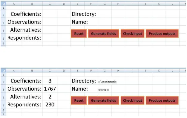
The macro-driven spreadsheet initialises to the situation shown in the first
half of Figure 1. Here, the user is required to specify the number of coefficients,
observations, alternatives and respondents. Additionally, an output directory needs to be specified, alongside a name for the model. In the second half of
Figure 1, we have used the settings from the empirical application in Section 3,
and have specified aconditionals subdirectory of the C drive along with naming
our modelexample.
Figure 1: Free software tool: initial settings (before and after)
The next step is for the user to press the Generate fields button. This produces
fields in which the user needs to enter respondent identification numbers, choice
2
www.stephanehess.me.uk
3
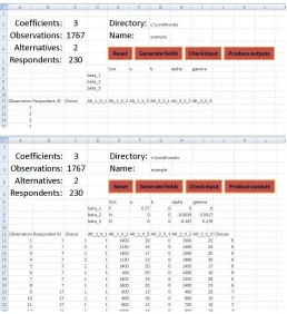
[image:6.612.161.474.366.564.2]Figure 2: Free software tool: data entry stage (before and after)
indicators and the attributes of the various alternatives4. Additionally, the
soft-ware generates a number of fields for each of the coefficients where the user needs to make a choice of distribution and enter the estimated parameters. A pop-up window explains the various settings to the user, and some explanations are also provided later in the paper in the context of the empirical application.
The situation after pressing the Generate fields button is illustrated in the
first half of Figure2. The second half shows the situation after the settings have
been entered. Here, the first parameter is a constant, fixed at 0.37, while the
travel time and travel cost coefficients follow Normal distributions, with means
and standard deviations given by theα and γ parameters, taken from the
appli-cation in Section 3. The spreadsheet is limited to coefficients using independent
Normal, Uniform, symmetrical Triangular, Lognormal and JohnsonSB
distribu-4
tions. These limitations however do not apply to the Matlab programme, and the user can also directly generate input files making use of other distributions, including multi-variate ones (e.g. multivariate Normal with Cholesky transfor-mation).
The figure shows all 8 choices for the first respondent, along with the first 3 choices for the second respondent. The attribute levels are entered in block for each alternative, using the same ordering as in the section specifying the coefficients. In the present example, the first attribute is a dummy variable used for the first alternative, with the second and third giving travel cost and travel
time respectively5.
The next two steps require the user to first run a check on the entered values (theCheck input button) before using theProduce outputs button to generate the input files for the Matlab programme. This latter button leads to the generation of three separate files, one containing the data, one containing the draws to be used for the various coefficients and one containing the settings of the problem in
terms of coefficients, observations, alternatives and respondents6. The file names
are based on the name specified by the user in cell G3.
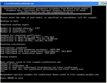
After completing the generation of the input files, the user is now ready to proceed to the Matlab tool for the computation of the conditional parameter estimates. After launching the executable, the user is prompted to enter the name of the model, as specified in cell G3 in the spreadsheet tool. The remainder
of the process requires no user input and is illustrated in Figure3. As a first step,
the software provides an overview of the data in terms of choices, respondents and coefficients. It then gives some summary statistics for the simulated draws for
the various coefficients. Finally, it shows the unconditional log-likelihood7, the
log-likelihood calculated with the conditional distributions for each respondent
(i.e. assigning the conditional weights from Equation1 to the individual draws),
and the log-likelihood calculated with the means of the conditional distributions for each respondent (i.e. making use of just one value for each respondent).
The software produces two output files8. The actual conditionals are saved in
a file that contains two columns for each coefficient, namely the mean and stan-dard deviation of the conditional distribution for each individual. Additionally,
5
Travel cost is given in øre, where one Danish Krone is equal to 100 øre, with travel time given in minutes.
6
If the inputs are generated manually, i.e. not making use of the spreadsheet, the user needs to similarly generate the appropriate three files.
7
Here, some discrepancies are possible when compared to the log-likelihood produced during estimation due to the use of different random draws. As an example, the unconditional and conditional log-likelihood values in Figure3differ slightly from those in Table1and Table2.
8
Figure 3: Free software tool: calculation of conditionals
the software produces a file that contains for each individual the weights for the
10,000 draws used as the input. The weights for a given draw from β, say βp,
is given by L(Yn|βp)
PR
r=1L(Yn|βr). On the basis of these weights, it is then possible to
produce draws from the conditional distribution for each respondent.
3
Empirical application
This section presents the findings of a brief application discussing the impacts of unconditional distributions on the shape of the conditional distributions. Model
estimation was carried out in Biogeme (Bierlaire,2005), making use of 500 Halton
which is only implemented with some parameter restrictions in NLogit.
3.1 Data
The analysis makes use of stated choice (SC) data collected for the DATIV study
carried out in Denmark in 2004 (cf. Burge and Rohr,2004). For this survey, a
binary unlabelled route choice experiment was used, with two attributes, travel time and travel cost describing the alternatives. For the present analysis, we
make use of 1,767 observations collected from 230 respondents.
3.2 Model specification
Across all models used, a constant was associated with the first alternative (δ1),
and the travel time (βTT) and travel cost (βTC) coefficients were interacted
lin-early with the associated attributes.
Depending on the specification of taste heterogeneity, up to four parameters
(a,b, α and γ) were estimated for each coefficient, where, in the context of this
illustrative example, univariate distributions were used. We will now look at the various models in turn.
MNL: In the MNL model, a point estimate (α) was estimated for both
coeffi-cients.
Uniform: In the MMNL model making use of a Uniform distribution, a left
boundary (a) was estimated along with a positive range parameter (b)9.
Triangular: In the MMNL model making use of a Triangular distribution, a left
boundary (a) was estimated along with a positive range parameter (b)10.
The distribution was constrained to be symmetrical, with the mean, median
and mode being equal to a+2b.
Normal: In the MMNL model making use of a Normal distribution, the mean
is given by α, with the standard deviation given by γ
Lognormal: In the MMNL model making use of a Lognormal distribution, α
andγ give the mean and standard deviation respectively for the underlying
Normal distribution. The offset parametera is either positive or negative,
and b is a direction parameter, which is equal to −1 for both coefficients,
resulting in a tail towards minus infinity.
9
Note that these parameters were obtained as transformations of the original Biogeme esti-mates which are for the mean and half the spread.
10
Johnson SB: In the MMNL model making use of a Johnson SB distribution,
α and γ again give the mean and standard deviation respectively for the
underlying Normal distribution. The offset parameter a is again either
positive or negative, andb is a positive range parameter.
3.3 Estimation results
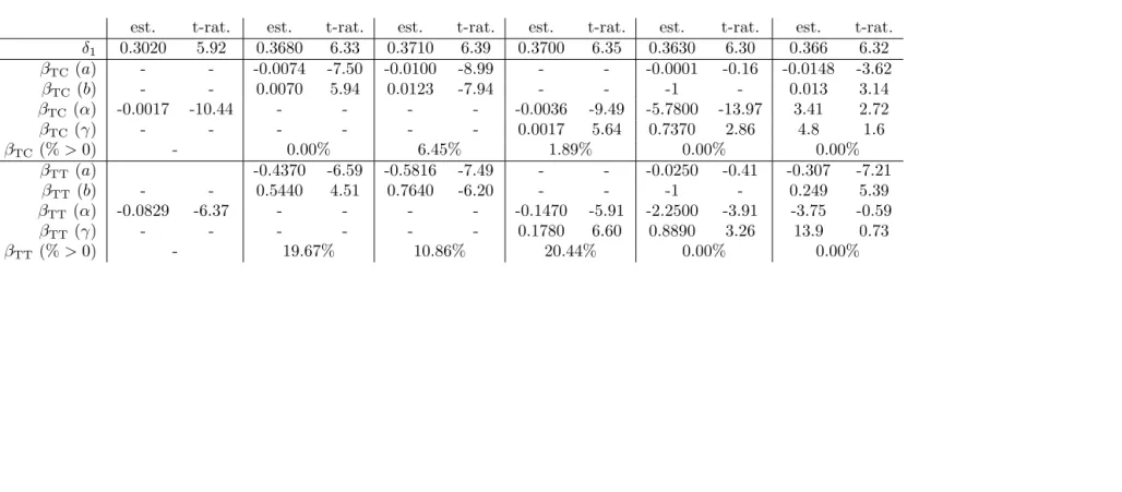
The estimation results are summarised in Table 1. Here, we can see that all
five MMNL specifications lead to significant gains in model fit over the MNL model, highlighting the presence of significant levels of taste heterogeneity in the
sample. In terms of the adjusted ρ2 measure, the best performance is obtained
by the Johnson SB distribution ahead of the Lognormal distribution, with the
symmetrical Triangular giving the poorest fit to the data. The three symmet-rical distributions produce significant probabilities of positive coefficient values,
especially forβTT, where these results can be directly linked to the distributional
assumptions (cf. Hess et al., 2005). Both the Lognormal and the Johnson SB
distributions indicate that the domain of the distribution for the two taste co-efficients should be entirely negative. Indeed, for the Lognormal distribution, both offset parameters are negative (albeit no different from zero), while for the
JohnsonSB distribution, the offset and range parameters are such that the
up-per limit for both coefficients is below zero. Before moving on, it should also
be noted that for the Johnson SB distribution, the second shape parameter (γ)
is only significantly different from zero at the 89% level for βTC, while for βTT,
neither shape parameter is significant at any reasonable level of confidence. This is an illustration of the difficulties of estimating parameters for this complex distribution.
3.4 Conditional model results
After estimation of the five MMNL models, the tool developed in Section 2 was
used to produce means and standard deviations for the conditional distributions for each respondent. As a first illustration of the additional information gained
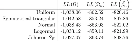
from this, Table 2 compares LL(Ω), the log-likelihood measures obtained
dur-ing estimation (i.e. usdur-ing the sample distribution parameters), to LL
ˆ
Ωn
, the log-likelihood measures obtained using the individual-specific conditional
distri-butions, and LL
ˆ
βn
, the log-likelihood measures obtained using the means of the conditional distributions.
Table 1: Estimation results
MNL Uniform Triangular Normal Logormal Johnson SB
Final LL -1,096.64 -1,038.06 -1,042.58 -1,038.43 -1,033.12 -1,027.07 Parameters 3 5 5 5 7 9
adj. ρ2 0.1020 0.1480 0.1447 0.1480 0.1510 0.1540
est. t-rat. est. t-rat. est. t-rat. est. t-rat. est. t-rat. est. t-rat.
δ1 0.3020 5.92 0.3680 6.33 0.3710 6.39 0.3700 6.35 0.3630 6.30 0.366 6.32 βTC(a) - - -0.0074 -7.50 -0.0100 -8.99 - - -0.0001 -0.16 -0.0148 -3.62
βTC (b) - - 0.0070 5.94 0.0123 -7.94 - - -1 - 0.013 3.14 βTC (α) -0.0017 -10.44 - - - - -0.0036 -9.49 -5.7800 -13.97 3.41 2.72 βTC (γ) - - - 0.0017 5.64 0.7370 2.86 4.8 1.6 βTC(%>0) - 0.00% 6.45% 1.89% 0.00% 0.00%
βTT(a) -0.4370 -6.59 -0.5816 -7.49 - - -0.0250 -0.41 -0.307 -7.21 βTT (b) - - 0.5440 4.51 0.7640 -6.20 - - -1 - 0.249 5.39 βTT (α) -0.0829 -6.37 - - - - -0.1470 -5.91 -2.2500 -3.91 -3.75 -0.59
βTT (γ) - - - 0.1780 6.60 0.8890 3.26 13.9 0.73 βTT(%>0) - 19.67% 10.86% 20.44% 0.00% 0.00%
Table 2: Log-likelihood at convergence and using conditional distributions, and means of conditional distributions
LL(Ω) LL(Ωn) LL
ˆ
βn
Uniform -1,038.06 -862.52 -820.46
Symmetrical triangular -1,042.58 -853.24 -807.86
Normal -1,038.43 -863.03 -822.02
Logormal -1,033.12 -859.11 -821.99
JohnsonSB -1,027.07 -863.74 -808.76
probabilities for each individual by drawing from a distribution for the random
coefficients that is more likely to be the true distribution for that respondent.
Further increases are obtained when relying solely on the means of the conditional distributions, i.e. using for each respondent the most likely values for the two coefficients.
Surprisingly, the best performance for the two conditional log-likelihood mea-sures is obtained by the Triangular distribution, even though it produced the
lowest log-likelihood measure in estimation (cf. Table 1). Furthermore, while
the JohnsonSB distribution obtained the best fit in estimation, it produces the
lowest measure for LL
ˆ
Ωn
, although, alongside with the Triangular distribu-tion, it then produces the best performance when working with the means of the
conditional distributions, i.e. LLβˆn
. This could suggest some differences in how well various distributions can be used to infer individual specific distribu-tions post estimation. However, it is not entirely clear what could be causing this interesting finding. A possible explanation could have been discrepancies between the unconditional distributions and the aggregated (over respondents) conditional distributions. As mentioned earlier, the aggregated conditional dis-tributions should be equal to the unconditional disdis-tributions. If for example, the
Uniform, Normal, Lognormal, and JohnsonSB distributions had failed that test,
this would have indicated that they are incorrect distributions for the present
application, unlike the Triangular11. However, all five distributions passed the
test, thus not indicating any inherent problems with one of the distributions, but rather supporting the above point about differences across distributions in the impact of the distributional assumptions on the conditional distributions.
As a first step in our comparison of the results across models, we look solely at the conditional means for the two coefficients, i.e. the most likely values for the
11
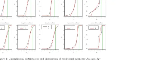
time and cost coefficients for each respondent. Empirical distribution functions
for the conditional means for the two coefficients are shown in Figure 4,
along-side the unconditional distributions. Here, we can see that for all five models, the distribution of the conditional means has a narrower range than the uncon-ditional distribution, where sign violations have also almost completely
disap-peared, repeating earlier results byGreene et al.(2005). For the cost coefficient,
the distribution has a significantly longer tail for the Lognormal and JohnsonSB
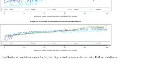
distributions, while, for the time coefficient, the ranges are more comparable. So far, we have looked at the empirical distribution function for the condi-tional means across respondents, and have compared these distributions across the five models. What is also interesting is to look at the results for each re-spondent separately and compare these across rere-spondents. This is the approach
taken in Figure 5, where, for clarity, the respondents are sorted according to
the conditional means produced by the Uniform model. This approach was used
solely with a view to analysing the stability across distributions in theordering of
conditional means, and as such, the specific choice of a base distribution should
have only limited impact. Here, we can see that forβTC, the results are relatively
stable for respondents with low cost sensitivity, while, for respondents with high cost sensitivity, the sensitivities produced by the Lognormal and especially the
JohnsonSB distribution are more extreme. ForβTT, the results are more stable
for respondents with high time sensitivity with the exception of the Lognormal distribution, while there is now a greater discrepancy across distributions when looking at respondents with low time sensitivity.
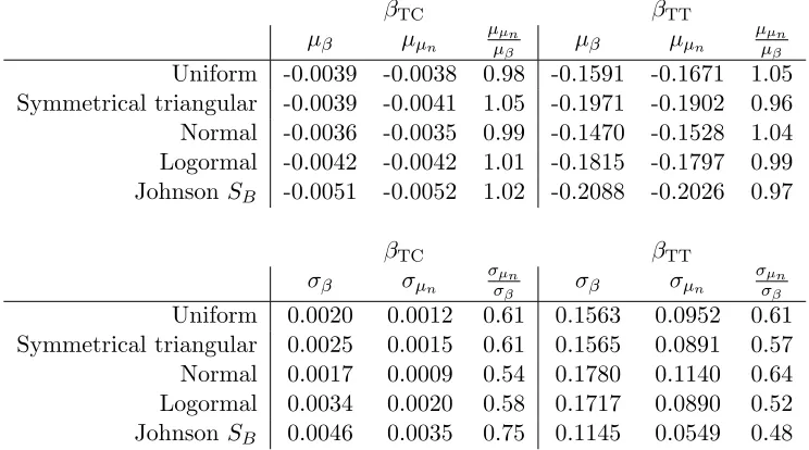
As a next step, we conduct an analysis similar to that reported inTrain(2003,
section 11.6.2.), by comparing measures of mean and standard deviation for the sample level distribution and for the distribution of the conditional means across respondents. The interest in this process is to see what share of the sample distribution variance is explained through making use of the conditional means only, hence disregarding any variation around these conditional means. The
results of this process are summarised in Table 3, where µβ and σβ refer to the
means and standard deviations of the estimated sample level distributions for the
two coefficients, andµµn and σµn refer to the means and standard deviations for
the distribution of the conditional means across respondents.
As expected for a well specified and consistently estimated model, there are
only very small differences between the sample distribution means (µβ) and the
means of the distribution of conditional means (µµn). Turning our attention to
the estimated standard deviations and the standard deviations for the distribu-tion of condidistribu-tional means across respondents, we observe major differences, with
σµn always being below σβ. This implies that not accounting for the
−0.015 −0.010 −0.005 0.000 0.005 0.0 0.2 0.4 0.6 0.8 1.0
Uniform cost coefficient
ββTC
F()
ββ ββn
^
−0.015 −0.010 −0.005 0.000 0.005
0.0 0.2 0.4 0.6 0.8 1.0
Triangular cost coefficient
ββTC
F()
ββ ββ^n
−0.015 −0.010 −0.005 0.000 0.005
0.0 0.2 0.4 0.6 0.8 1.0
Normal cost coefficient
ββTC
F()
ββ ββ^n
−0.015 −0.010 −0.005 0.000 0.005
0.0 0.2 0.4 0.6 0.8 1.0
Lognormal cost coefficient
ββTC
F()
ββ ββn
^
−0.015 −0.010 −0.005 0.000 0.005
0.0 0.2 0.4 0.6 0.8 1.0
Johnson SB cost coefficient
ββTC
F()
ββ ββ^n
−1.0 −0.8 −0.6 −0.4 −0.2 0.0 0.2
0.0 0.2 0.4 0.6 0.8 1.0
Uniform time coefficient
ββTC
F()
ββ ββn
^
−1.0 −0.8 −0.6 −0.4 −0.2 0.0 0.2
0.0 0.2 0.4 0.6 0.8 1.0
Triangular time coefficient
ββTC
F()
ββ ββ^n
−1.0 −0.8 −0.6 −0.4 −0.2 0.0 0.2
0.0 0.2 0.4 0.6 0.8 1.0
Normal time coefficient
ββTC
F()
ββ ββ^n
−1.0 −0.8 −0.6 −0.4 −0.2 0.0 0.2
0.0 0.2 0.4 0.6 0.8 1.0
Lognormal time coefficient
ββTC
F()
ββ ββn
^
−1.0 −0.8 −0.6 −0.4 −0.2 0.0 0.2
0.0 0.2 0.4 0.6 0.8 1.0
Johnson SB time coefficient
ββTC
F()
[image:15.612.140.638.163.442.2]ββ ββ^n
Figure 4: Unconditional distributions and distribution of conditional means forβTC and βTT
−0.015
−0.010
−0.005
0.000
Comparison of conditional means for cost coefficient with different distributions
Respondents, sorted by conditional mean for cost coefficient with Uniform distribution ββTC
1 45 90 135 180 230
Uniform Triangular Normal Lognormal Johnson SB
−0.6
−0.4
−0.2
0.0
Comparison of conditional means for time coefficient with different distributions
Respondents, sorted by conditional mean for time coefficient with Uniform distribution ββTT
1 45 90 135 180 230
[image:16.612.126.640.172.442.2]Uniform Triangular Normal Lognormal Johnson SB
Figure 5: Distribution of conditional means forβTC andβTT, sorted by values obtained with Uniform distribution
Table 3: Mean and standard deviation for sample level distributions and for distribution of conditional means
βTC βTT
µβ µµn
µµn
µβ µβ µµn
µµn
µβ
Uniform -0.0039 -0.0038 0.98 -0.1591 -0.1671 1.05
Symmetrical triangular -0.0039 -0.0041 1.05 -0.1971 -0.1902 0.96
Normal -0.0036 -0.0035 0.99 -0.1470 -0.1528 1.04
Logormal -0.0042 -0.0042 1.01 -0.1815 -0.1797 0.99
JohnsonSB -0.0051 -0.0052 1.02 -0.2088 -0.2026 0.97
βTC βTT
σβ σµn
σµn
σβ σβ σµn
σµn σβ
Uniform 0.0020 0.0012 0.61 0.1563 0.0952 0.61
Symmetrical triangular 0.0025 0.0015 0.61 0.1565 0.0891 0.57
Normal 0.0017 0.0009 0.54 0.1780 0.1140 0.64
Logormal 0.0034 0.0020 0.58 0.1717 0.0890 0.52
JohnsonSB 0.0046 0.0035 0.75 0.1145 0.0549 0.48
heterogeneity in the data. There are some differences across distributions, but on average, we can see that making use of only the conditional means, we recover just over half the sample level heterogeneity. This means that the share of the differences across respondents that is captured through making use of the means of the conditional distribution is in this case potentially large enough to allow us to use this information to distinguish between respondents, for example in cluster analysis. However, it also means that the individual specific coefficient values are not known with certainty (in which case the standard deviation of the distribu-tion of condidistribu-tional means would be equal to the sample level standard deviadistribu-tion), and that it would hence not be adequate to make use of these conditional means for example in the calculation of willingness to pay measures.
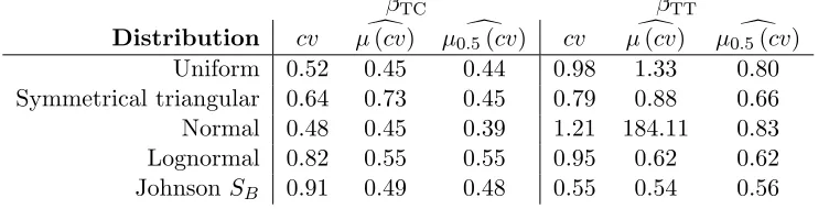
un-Table 4: Degree of heterogeneity expressed as coefficient of variation
βTC βTT
Distribution cv µd(cv) µ0.d5(cv) cv µd(cv) µ0.d5(cv)
Uniform 0.52 0.45 0.44 0.98 1.33 0.80
Symmetrical triangular 0.64 0.73 0.45 0.79 0.88 0.66
Normal 0.48 0.45 0.39 1.21 184.11 0.83
Lognormal 0.82 0.55 0.55 0.95 0.62 0.62
JohnsonSB 0.91 0.49 0.48 0.55 0.54 0.56
dertake this comparison by calculating the coefficient of variation for βTC and
βTT for each respondent. The results of this process are summarised in Table
4. Here, we show three measures for each coefficient, namely the coefficient of
variation of the unconditional distribution (cv), the mean across respondents of
the coefficient of variation for the conditional distributions (µd(cv)) and the
cor-responding median (µ0.d5(cv)). The reason for including the latter is that it is
less sensitive to outliers. Looking first at the travel cost coefficient, we see sig-nificant differences across estimated distributions, with much higher variation for
the Lognormal and Johnson SB distributions. When looking at the conditional
distributions, especially in terms of the median, the results are far more stable across the five distributions. Turning our attention to the travel time coefficient, the main outliers when looking at the unconditional distributions are the
Nor-mal (high) and the Johnson SB (low). With the conditional distributions, the
results are again more similar, though only when working with the median given the huge outliers with the Normal distribution that have a major impact on the mean. Comparing the median of the coefficient of variation for the conditional
distributionµ0.d5(cv)) to the coefficient of variation for the sample level
distribu-tion (cv), we observe, with the exception of the JohnsonSB forβTT, a reduction
in the degree of heterogeneity. This is consistent with the observation in Table
3 that part of the heterogeneity is captured in the variation across respondents
in the conditional means, where this share of the heterogeneity is lowest for the
JohnsonSB forβTT.
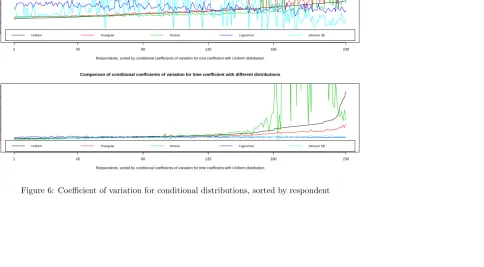
As a final step, Figure6shows a graphical analysis of the results summarised
in Table4where we again sort the result by respondent according to the measures
obtained with the Uniform models. Here, we can see significant differences across the five distributions especially for respondents with high degrees of uncertainty in the conditional distributions, with the biggest outliers arising from the Triangular and Normal models. This also shows the large differences across respondents
[image:18.612.132.508.155.250.2]Comparison of conditional coefficients of variation for cost coefficient with different distributions
Respondents, sorted by conditional coefficients of variation for cost coefficient with Uniform distribution
cv
T
C
1 45 90 135 180 230
0.0
0.2
0.4
0.6
0.8
1.0
1.2
Uniform Triangular Normal Lognormal Johnson SB
Comparison of conditional coefficients of variation for time coefficient with different distributions
Respondents, sorted by conditional coefficients of variation for time coefficient with Uniform distribution
cv
T
C
1 45 90 135 180 230
0
2
4
6
8
10
[image:19.612.128.635.168.435.2]Uniform Triangular Normal Lognormal Johnson SB
Figure 6: Coefficient of variation for conditional distributions, sorted by respondent
the time coefficient, with even bigger discrepancies for respondents with high
degrees of uncertainty. In contrast with Figure5, this shows that while the results
are quite stable across distributions in terms of the means of the conditional distributions, i.e. the most likely location of each respondent on the sample level distribution, differences arise in the variation around these mean levels. This is also consistent with an observation that can be made for the unconditional
distributions on the basis of Table 3, namely that while the mean values are
relatively stable across the five distributions, there are much larger differences when it comes to the retrieved degree of heterogeneity.
4
Summary and conclusions
This paper has discussed the issue of the computation of conditional distribu-tions for coefficients estimated using continuous Mixed Multinomial Logit mod-els. While this topic has been looked at at length by various authors, as discussed
in Section 1, the number of applications making use of conditional distributions
is still relatively limited. This paper has identified the lack of available software
(other than NLogit, Econometric Software 2007) as one reason for this and has
consequently discussed the development of a freeware software tool that allows users to compute conditional distributions from any choice of unconditional
dis-tributions12, independently of the software used during model estimation.
The paper has also looked at an additional issue in this area, namely the im-pact of assumptions made for the unconditional distributions on the shape of the conditional distributions. Here, an application using stated choice data collected in Denmark has shown that while the move from unconditional to conditional distributions potentially brings results closer together (notably in terms of the conditional means), some discrepancies do remain. In this context, further work is required, notably a large scale study making use of simulated data with various
underlyingtruedistributions. It is also important to acknowledge a limitation of
the present study in that it does not take into account the sampling distribution of the parameters of the underlying distribution, a further development in the
context of conditional distributions, discussed byTrain(2003, section 11.3).
Acknowledgements
This paper is based on work funded by a University of Leeds Knowledge Trans-fer grant, with further developments undertaken thanks to a Leverhulme Early
12
Career Fellowship. The inspiration for the empirical analysis stems from earlier work conducted with John Rose in the Institute of Transport and Logistics Stud-ies at the University of Sydney. The author would also like to thank Richard Connors for coding suggestions, and Kenneth Train for useful feedback.
References
Bierlaire, M., 2005. An introduction to BIOGEME Version 1.4. biogeme.epfl.ch.
Burge, P., Rohr, C., 2004. DATIV: SP Design: Proposed approach for pilot survey. Tetra-Plan in cooperation with RAND Europe and Gallup A/S.
Campbell, D., Hess, S., 2009. Outlying sensitivities in discrete choice data: causes, consequences and remedies. paper presented at the European Transport Conference, Noordwijkerhout, The Netherlands.
Econometric Software, 2007. Nlogit 4.0. Econometric Software, New York and Sydney.
Fosgerau, M., 2006. Investigating the distribution of the value of travel time savings. Transportation Research Part B 40 (8), 688–707.
Greene, W. H., Hensher, D. A., Rose, J. M., 2005. Using classical simulation-based estimators to estimate individual wtp values. In: Scarpa, R., Alberini, A. (Eds.), Applications of Simulation Methods in Environmental and Resource Economics. Springer Publisher, Dordrecht, Ch. 2, pp. 17–33.
Hensher, D. A., Greene, W. H., 2003. The Mixed Logit Model: The State of Practice. Transportation 30 (2), 133–176.
Hess, S., 2007. Posterior analysis of random taste coefficients in air travel choice behaviour modelling. Journal of Air Transport Management 13 (4), 203–212.
Hess, S., Bierlaire, M., Polak, J. W., 2005. Estimation of value of travel-time savings using mixed logit models. Transportation Research Part A 39 (2-3), 221–236.
Hess, S., Hensher, D. A., 2008. Using conditioning on observed choices to re-trieve individual-specific attribute processing strategies. paper submitted to Transportation Research B.
Revelt, D., Train, K., 1998. Mixed Logit with repeated choices: households’ choices of appliance efficiency level. Review of Economics and Statistics 80 (4), 647–657.
Revelt, D., Train, K., 1999. Customer-specific taste parameters and Mixed Logit: Households’ choice of electricity supplier. Working Paper No. E00-274. Depart-ment of Economics, University of California, Berkeley, CA.
Sillano, M., Ort´uzar, J. de D., 2004. Willingness-to-pay estimation from mixed
logit models: some new evidence. Environment & Planning A 37 (3), 525–550.
Train, K., 1998. Recreation demand models with taste differences over people. Land Economics 74, 185–194.
Train, K., 2003. Discrete Choice Methods with Simulation. Cambridge University Press, Cambridge, MA.