Mark Russell Upcher
A t h e s i s s u b m i t t e d t o the A u s t r a l i a n N a t i o n a l U n i v e r s i t y f o r the degree o f Do ct or o f P h il osophy
In this thesis further consideration is given to the theory and
application of disequilibrium models in econometrics. Since the important work by Fair and Jaffee (1972) there has been a substantial body of
literature dealing with this topic. Typically much of this research has been devoted to increasing knowledge about the estimation techniques for these models and applications are less common. An analysis of the Official Short Term Money Market attempts to redress this imbalance and to show how a disequilibrium approach has the potential to enrich the specification of a model. However, before proceeding with this application a number of
theoretical issues arc considered. Firstly, the economic framework of
disequilibrium models is considered, especially where it has an influence on the econometric framework. It is a weakness in some applications that closer attention is not paid to the economic aspects of disequilibrium in the
markets under consideration.
While estimation of models of markets in disequilibrium is well
established in the literature, there arc some issues not dealt with entirely adequately, and where this is the case an attempt at resolution is made.
Some of these issues lead on to a simulation study of three stage instrumental variables estimators. Also examination of estimation techniques indicate problems in estimating some disequilibrium specifications and so the Score test is examined as a means of avoiding estimation of disequilibrium models whenever possible, by using a test based on equilibrium estimates.
ACKNOWLEDGEMENTS i
ABSTRACT ii
CHAPTER 1 TUE THEORY OF DISEQUILIBRIUM 1
1.1 Introduction 1
1.2 Approaches to the Modelling of Disequilibrium 9 1.3 Disequilibrium Analysis in a Multimarket Framework 22
1.4 Conclusion 29
CHAPTER 2 THE THEORY OF ESTIMATION OF MARKETS IN DISEQUILIBRIUM 30
2.1 Introduction and Notation 30
2.2 The Directional Method of Estimation 33
2.3 Least Squares Estimation of Models with a
Walrasian Equation 36
2.4 Maximum Likelihood Estimation of Models with a
Walrasian Equation 58
2.5 Conclusion 74
CHAPTER 3 A MONTE CARLO STUDY OF LEAST SQUARES ESTIMATION IN
DISEQUILIBRIUM MODELS 75
3.1 Introduction 75
3.2 The Model Used for Simulation 78
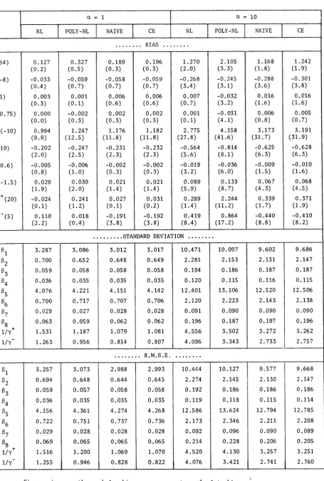
3.3 Simulation Results 79
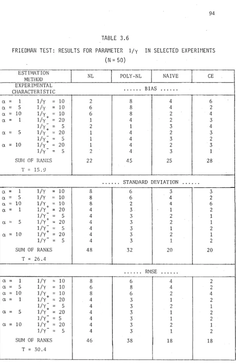
3.4 Simulation of an Alternative Model 95
3.5 Conclusion 96
CHAPTER 4 THE SCORE TEST FOR MARKETS IN DISEQUILIBRIUM 99
4.1 Introduction 99
4.2 A Disequilibrium Model with Non-Stochastic Adjustment 104
4.6 Conclusion 110
CHAPTER 5 A DISEQUILIBRIUM MODEL OF THE OFFICIAL SHORT TERM
MONEY MARKET 120
5.1 The Operations of the Official Short Term Money
Market 120
5.2 The Motivation of the Disequilibrium Approach to the
Modelling of the Market 122
5.3 The Demand and Supply Relationships of the OSTMM
Model 129
5.4 Disequilibrium in the Official Short Term Money
Market 147
5.5 Estimation of the Model 150
5.6 Hypothesis Testing in the OSTMM Model 158
5.7 Conclusion 163
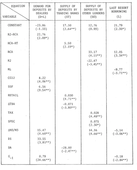
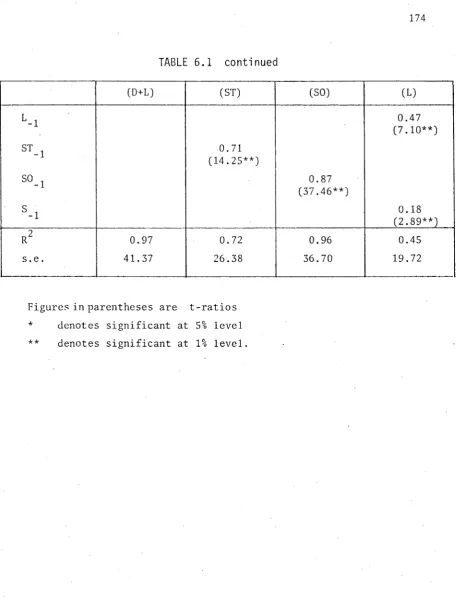
CHAPTER 6 THE ESTIMATION OF THE MODEL OF THE OFFICIAL SHORT
TERM MONEY MARKET 164
6.1 Introduction 164
6.2 The Data Used in the Model 165
6.3 The Optimization Procedure for Maximum Likelihood
Estimation 169
6.4 Preliminary Estimation: The Equilibrium Hypothesis 171 6.5 The Disequilibrium Model: Least Squares Estimation 180 6.6 Maximum Likelihood Estimation of the Basic Walrasian
Specification 191
6.7 Maximum Likelihood Estimation of the Stochastic
Walrasian Specification 203
6.8 Conclusions 206
Appendix 209
CHAPTER 7 SUMMARY AND CONCLUSIONS 211
C H A P T E R 1
THE T H E O R Y OF D I S E Q U I L I B R I U M
1.1 I N T R O D U C T I O N
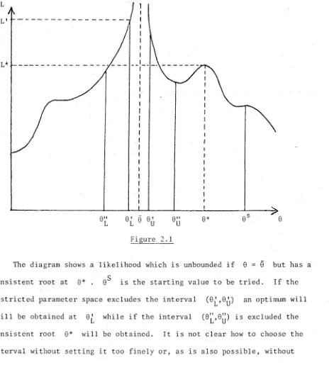
Disequilibrium is a word that lias been used to describe many behavioural phenomena in economic theory, so much so, that it is worthwhile considering such phenomena and attempting to establish some criteria for distinguishing between behaviour that might be regarded as consistent with equilibrium and that which might be best described as disequilibrium behaviour. Because the term disequilibrium has been used to encompass so many different aspects of economic behaviour, a useful starting point is to provide a very general definition.
The Oxford English Dictionary (1969) describes disequilibrium as the "... absence or destruction of equilibrium..."1 and describes equilibrium as "... the state of equal balance between powers of any kind..."2. This is a very general definition of equilibrium. IVebsters (1976) provide a more specific definition: "... a ... position toward which economic forces impel or about which fluctuations occur..."3.
Assuming that a decision maker attempts to reach this state of balance the question often arises as to the dynamic process involved4 . One argument
1 The Oxford English Dictionary, Oxford University Press, Vol. Ill, 1969, p.446.
2 The Oxford English Dictionary, op.cit., p.257.
3 IVebsters Third New International Dictionary, G. f, C. Mcrrian T, Co., Massachusetts, 1976, p.768.
usual approach being to distinguish between different types of equilibrium (such as long run and short run).
At the centre of most economics is a choice theoretic structure in which decision makers attempt to optimize some objective function subject to
constraints. The solution to this optimization problem is based on information available about the items or goods in the choice set. In a market economy the most important information is that of price. Given a vector of prices and initial endowments,the decision makers attempt to obtain the desired bundle of goods by trade in the various markets. As this trade takes place it is likely that the price vector will change,in which case the decision makers also revise their choices. It is a feature of an equilibrium model that such revisions take place quickly (instaneously) so that at no stage are decision makers forced into the position of not being able to satisfy their desires at the prevailing prices. Thus the state of balance is being continuously
attained, with fluctuations about that state never being observed.
position; if they are not at the long-run equilibrium it is because they have chosen not to be there. More will be said about this in the next section.
The next development to be considered is that of the Walrasian equation explaining dynamic price adjustment. The equation evolves from the reasonable assumption that prices rise in response to excess demand and fall in response to excess supply. Samuelson (1941) writes this more precisely as:
(1.1) p = ^7 = H(q^-q^) where 11(0) = 0 and II' > 0 .
However it is still possible to regard (1.1) as simply an artifice designed to describe the behaviour of an auctioneer who "... registers the buy and sell offers. If .... there is excess demand, a higher price is called out; if excess supply is registered, a lower price is tried. The process is repeated until a market clearing price is found. Only then are actual
exchanges allowed to he carried out... Such markets always clear ..."5.
In the continuous time framework this means the tatonnement process is instantaneous; if the model is in discrete time the process occurs between one period and the next. As pointed out by Leijonhufvud no transactor faces quantity constraints at the market price nor arc they required to find terms for themselves.
With the work by Clowcr (1965), Leijonhufvud (1968) and Alchian (1970), the possibility of non-clearing markets has been given a stronger basis. The essential feature of such a notion is that information on the best
obtainable price is not available instantaneously or at zero cost to the individual transactor. In such cases it is optimal for a transactor to carry out a search for a favourable price and it may be preferable to do so "... while the good or person is not employed, and thus able to specialize... in the production of information"6 . Some transactions will take place as the market moves gradually toward the new market clearing position and so
equation (1.1) will now represent observable behaviour (manifested, for
example, by labour market unemployment or commodity market inventory changes). To make the search and information cost analysis completely logical, the
assumption in atomistic markets that all transactors are price takers is replaced by one that some traders have the option of making price offers and so are transitorily monopolists or monopsonists when the market does not clear, this power disappearing when all traders have full information at their disposal7. Thus there are transactors, usually either the sellers or the buyers, actually making a decision on price. Finally, Gordon and Hynes (1970) have indicated that the continuous time formulation with a perfectly divisible commodity would imply search is instantaneous and costless, in which case markets will always clear. This means that the individual's decision process is better formulated in a discrete time framework. If the various individuals make decisions at different moments then aggregation may lead to acceptance of the continuous time formulation of equation (1.1); however, when analysing economic data, observations are only available at discrete time intervals, so for practical considerations the discrete form:
( 1 . 2 ) Apt = p t - p t _x = l l ( q D t - q S t ) ; 11(0) = 0 , 11' > 0
is preferred.
6 7
Alchian (1970), p.110.
Having argued for the possibility of non-clearing markets, the question arises as to the determination of actual quantity observed. It is possible to make no assumptions about this so that actual quantity remains
indeterminate. Bowden ((1978a), chapter 3) examines such a model. However it has been more common to make additional assumptions which are usually of the general form:
(1.3)
with k Dt
> ks t e
made:
(i) kDt + k: p .498) .
If kDt ’
(ii) kDt + k;
aid kDt = k(qDt-,
= kDt ’ V + kSt ‘ ‘'St
St
St 1 , kt = k(xt)
or
c*t
qs t
1 if X V o t 0 if xt > o
Jaffee (1972):
( 1 ' 4) l' t = mi n ( qD t . q s P
which is just a special case of (i).
(iii) kDt + kSt = ß £ 1 ’ kt = k(xd =
and kp^ = k^pt'^St^ fivcs the condition
0 if xt < o 0 if x > 0
C1-5)
qt
^ min(qnt»qSt)as proposed by Muellbauer (1978).
adopts a slightly different approach by writing:
(1.6)
(1.7)
y S ’ PS ~ 0 '
(1.8)
If a , 3 , C are all non-zero (1.5) is obtained while if a = 1 , 3 = 1
and C = 0 then (1.4) is obtained. This approach has advantages in
considering multimarkct models discussed in section 1.3 and in handling the
likelihood for particular disequilibrium models discussed in chapter 2.
In each of the examples given, the actual quantity traded will differ
from the notional quantity demanded and/or the notional quantity supplied.
The result of this may be unexpected inventory changes or quantity rationing
of one side of the market (or possibly both). Y.'hile major interest in this
thesis is focussed on the type of model with a dynamic price adjustment
equation like (1.2) and some scheme determining quantity of the general form
(1.3), it is worth noting that alternative approaches are often available.
If either quantity produced or traded plus inventory levels arc observed, it
is often possible to build a model in which suppliers determine price, output
and desired inventory levels while buyers determine quantity demanded at that
price. The difference between actual output and demand will be reflected by
inventory changes, some portion of which may be undesired8 . In economic
modelling this approach, when possible, may bypass problems associated with
the alternative that does not, or cannot, account for inventories and instead
uses (1.2) and (1.3) together with notional demand and supply curves. In
The disequilibrium model to be examined in greatest detail from section 1.2.3 onwards consists of the following equations in the case of a single market:
(1.9)
Dt = D(pt,Xlt)
(1.10) ' St = S(pt ,x2t)
(1.11) Apt = ll(Dt-St)
(1.12) Qt = min(Dt ,St)
where D, is quantity demanded, Sf quantity supplied, X and X^ vectors of exogenous demand and supply variables, 0^ is actual quantity traded and p is price, all variables being observed at time t . Such a model will be of value in econometric modelling when it is suspected that market clearing is sufficiently slow to occur, enabling non-clearing prices and quantities to be observed, and when information on inventories is
unavailable. On economic grounds this type of model is ad hoc but a rigorous explanation of market search introducing costs of acquiring information into the decision makers utility function (in the short run only) has yet to be developed. A model that includes these factors will fall within the
In trying to define disequilibrium, it becomes apparent that it can be defined out of existence as one modifies the definition of equilibrium to account for new categories of costs previously not considered. Once adjust ment costs are allowed for, the generalized (or partial) adjustment model can be termed an equilibrium model with the equilibrium position changing over time. If economic theory introduced search costs and information into the choice theory an equilibrium model would replace the disequilibrium model (1.9) - (1.12). This would leave random fluctuations as the only
source of true disequilibrium, with any other behaviour completely explicable given all costs, prices and initial endowments. In the absence of this
framework the behaviour embodied in a system such as (1.9) - (1.12) is hereafter regarded as disequilibrium behaviour. To the extent that many models such as generalized (or partial) adjustment models have an underlying framework they will be termed equilibrium models. However since it is
possible for these models also to be derived from equations (1.9) - (1.12), they are of significance when considering disequilibrium models.
1 . 2 A P P R O A C H E S T O T H E M O D E L L I N G O F D I S E Q U I L I B R I U M
1 . 2 . 1 P a r t i a l a n d G e n e r a l i z e d A d j u s t m e n t M o d e l s
An assumption of partial adjustment is very commonly included in
economic models. That is:
U-13) yt ' yt-i = 5(y^-yt_i)
where y* is the long run desired level of y at time t and is usually
some function of other variables:
(1.14)
The quadratic adjustment and disequilibrium cost framework underlying (1.13)
is well known and not repeated h e r e 9 . However it is worth noting that the
quadratic disequilibrium costs, which are designed to account for profit or
utility foregone as a result of being away from the long-run desired
position, are only an approximation. To avoid this approximation a better
derivation of the partial adjustment process is to include adjustment costs
in the original utility function. For example:
(1.15) v r
- t t
b 2 2
2 G R yt
I
( y t - y t - dwhere r^ is the rate of return on the activity under consideration,
the variance of r , b and c are positive parameters. Then maximization
y i e l d s :
cy
(1.16) t-1
bo^+c
b0 R+C
which is the same as first maximizing y r^. b 2 2
2 °R>t to obtain y* and
then forming
(1.17)
c
= <y;-yt)rt - +1 C v W 2
and minimizing C . The first two terms represent utility foregone as a result of y* ^ y . By using (1.15) and (1.16) it is clear that y* is a contrivance, since only if c = 0 is y* ever chosen in period t . The decision maker correctly accounting for all benefits and costs (rate of return, risk, adjustment costs) and initial conditions chooses y^ to maximize current profit or utility. In this respect partial adjustment models may still be classified as equilibrium models.
However the system (1.9) - (1.11) (i.e. (1.12) excluded) can lie used to derive a partial adjustment equation (provided D , S and II are replaced by linear functions of right hand side variables). This is the basis of the PAMEQ specification suggested by Bowden (19’78a, 1978b) :
(1.18) pt = pp£ + (l-y)pt_l 0 < p < 1
which is an alternative to (1.11) and is sometimes much easier to interpret c
(see section 2.5.1). The other equation in this model explains p by solving (1.9) and (1.10):
(1.19)
p® = nzt
where II depends on the structural parameters of demand and supply curves and Z. includes all the variables in X^ and X„
t It 2t
is of the form:
(1.20) Bx
t
(1.21) Ayt = D(y*-yt _])
where yt is a vector of observed endogenous variables, x^. is a vector of
exogenous variables, and B and D are matrices of appropriate conform-
ability. Equations (1.20) and (1.21) are combined as:
where C = DB and A = I - D and this is the type of model usually
estimated in econometric applications. Hunt and Upcher (1979) show that
a model of this form,based on quadratic adjustment and disequilibrium costs,
must be stable and also show how standard errors of the eigenvalues of the
system can be obtained to test for stability. If the modification suggested
in (1.15) for the scalar case is adopted for the vector case the stability
property can be verified just as before10. As mentioned before these models
can be regarded as equilibrium models with adjustment via short-run
equilibria to a long-run equilibrium.
The vector generalization can also be used for a multimarket PAMEQ
specification:*11
where if P is a k x 1 vector of prices and a G x 1 vector of
10 See Hunt and Upcher (1979), pp.313-317.
11 See Bowden (1978a), chapter 3.
(
1.
22)
(1.23) p t = MPj; + (I-M)Pt _]
(1.24) P® = BZ
exogenous variables then M is k x k and B is k * G .
The problem with models of the form (1.18) - (1.19) or (1.23) - (1.24) is that the quantity traded is left unexplained and the exogenous variables
cannot be separated into demand determining or supply determining
variables in any way unless the model builder has strong a priori grounds for particular classifications. Additional information in a model or
additional assumptions may be desirable to overcome these problems. This is essentially the approach used in the models in the next two sections.
1 . 2 . 2 T h e R o l e o f A d d i t i o n a l I n f o r m a t i o n
There are a significant group of models where the presence of disequilibrium, as manifested by inequality between notional demand and notional supply, can be handled by using stock-flow models where information on inventories or unemployed resources is available. For example Muellbauer
(1978), Bowden (1978a) and Kooiman and Kloek (1979) have worked in the
labour market context where unemployment and vacancies are used as indicators of market disequilibrium. However their treatment, while of value in explain ing the familiar unemployment-vacancies trade-off, may be recast to obtain the underlying supply of labour and demand for labour functions so that they can be estimated normally. That is, given employment, N , unemployment, Ut , and vacancies, , real wage, w^/p , and supply and demand exogenous variables and the model may be set up as:
( l - 2 5)
L st - N t ♦ U t = Ls ( w t / p t ,Xs t )
u-26)
St = Nt +
h ■
W v T d
demand model. This is an oversimplification in reality, since unemployment and vacancies are rarely accurately collected and some of the stock of
unemployed labour is outside the workforce but able to move in very readily. Also unemployment and vacancies are collected as numbers of people or numbers of jobs while employment is more correctly measured as total manhours.
Models of commodity markets may also may also make use of inventories to avoid using a disequilibrium model. For example a supplier may be able to set price (at least in the short run), output and desired inventories. If price is set according to the supplier's perception of the demand curve the output-inventories decision may be inconsistent with the quantity demanded. However, if inventories are observed, the difference between output and quantity traded is observable using the identity:
(1.27) xt =
Q t + A It
where X^ is output, Qt quantity traded and I inventories. Observing Qt enables X to be deduced or vice versa. This is under an assumption that producers never close up shop when declines in inventory become
excessive or never ration buyers, for example, by only selling to regular customers. If such behaviour is possible or if inventory observations are unavailable then the use of additional assumptions,such as the addition of
(1.11) and (1.12) to the equations (1.9) and (1.10), becomes useful.
1. 2. 3 The D i s e q u i l i b r i u m Model
In this section the disequilibrium model (1.9) - (1.12) will be
singled out for specific attention. Since the other equations cause little difficulty they are considered first.
The demand and supply relationships of the model can be derived from choice theory assuming no monopoly or monopsony power - that is, all
transactors are price takers. They can be regarded as notional supply and demand relationships, determining notional equilibrium price and quantity, and can even include lagged quantities (partial adjustment),12 although the choice between lagged notional and lagged effective quantities is one which has considerable implications for estimation of the model, as demonstrated later in this section and in section 2.3.1. At this point imposition of the condition:
(1.28)
Qt = °t =
Stwould result in an equilibrium model13. However instead it is assumed that if one of the curves shifts then the necessity for market search imposes short term costs on decision makers. As information is assimilated there is a gradual movement back to equilibrium as implied by (1.28); meanwhile the short side of the market determines quantity traded thus giving rise to the minimum condition (1.12).
Now turn to the actual adjustment process. Assume that in the short run each firm has the ability to quote prices in response to observed imbalances in quantity demanded and supplied but has no overall monopoly
12 The incorporation of lagged variables can overcome the problem of the
model suggesting that in response to a fall in demand quantity traded first falls then rises. This problem is demonstrated by Chow (1977). 13 The equilibrium model if solved will show price and quantity as a
function of lagged quantity in the case where lagged quantity is
power. Some suppliers quote above the competitive price, others below, but
within a certain band. Outside this band, a high price results in the
supplier gaining no additional trade while a low price results in the
supplier being swamped by additional buyers. The overall effect is assumed
to be that suppliers are at some point on the aggregate supply curve.
However movement toward the equilibrium will not be instantaneous because
disequilibrium costs and future search costs are offset by adjustment costs
and present search costs. Assuming quadratic costs the adjustment and
current search costs will depend on the magnitude of the movement from the
original position to the current short run position. The disequilibrium
and future search costs will depend on the magnitude of the adjustment that
still remains. Thus:
a - 29) Ct = I
(St-st_ p
2
♦
I(Dt.r s
t)2
which is minimized with respect to S .
3C 1
That is = a(St -S^ ^) - b(Dt _^-S^_) = 0 . The solution is
(1.30) + — — Sa c
a+b t-1 a+b t-1
which can be written as:
(1.31)
A - h-i
a+b (D t-1,-S ,)The first thing to note is the similarity of (1.30) to a partial adjustment
process, but with S* replaced by D ^ . Next, if it is assumed that the
supply curve is of the form:
(1.32)
st = s (i’ 0
(1.33)
S(>V - sfPt-P =
(D
or
(1.34)
But this is just a Walrasian equation with price adjustment to lagged
disequilibrium as has been suggested by Laffont and Monfort (1977). The
interval between successive observations may in practice make the version
depending on current disequilibrium more appropriate. In econometric
studies the choice between (1.11) and (1.34) may be set up as a choice
between competing hypotheses although one may be ruled out on a priori
grounds.
To the extent that the adjustment costs may depend on other variables
that affect the supplier it may be feasible to respecify (1.11) as:
For example in certain circumstances if a new production technique is
available it may mean that rather than increasing output and supply by
increasing employment a more lengthy adjustment process involving new
capital may be chosen. However,in general the property 11(0,Xp ) = 0 should
be maintained as it is logical to expect no price variation when equilibrium
is attained. One possible exception to this is administered pricing
schemes where a central authority sets prices "... perhaps with a
genuflection to the current state of demand"14. Another is where an
oligopolist sets price as a mark-up on average costs, with the state of demand
having a secondary effect. These situations are allowed for when issues
concerning estimation of disequilibrium models are discussed in chapter 2 (1.35)
A p t = " (t fV PtW •
but for the application in chapters 5 and 6 there are a priori reasons for forcing this function to pass through the origin.
In the original work by Fair and Jaffce (1972) it is argued that the price variable appearing in the functions should be the relative price of the good, i.e. the actual price normalized by a general price index (p.498). This argument may be based on the fact that in a general equilibrium
consumption model it is only relative prices that are important. Apart from the effect of the particular price on the general price index, usually
sufficiently negligible, the general price index is exogenous to the
particular market. Write as the price level of the particular good and as the general price index so that relative price is P^/G^. (=pt) . If G rises as a result of general inflation and P^ does not rise at the same rate then P /Ci < P /G but ceteris paribus I) > S. due to the
t t t - l t - 1 t t
slopes of the demand and supply curves. This is in direct contradiction with (1.11). Therefore it must be the case that in response to a change in Gj. , P^ also changes in such a way that p (=P^./Gt) does not change and Df = S is maintained. This means it must be assumed that the response of the price level to the general price index is instantaneous with no
disequilibrium resulting. Unless G^ is also included separately in demand and/or supply equations the existence of short-run money illusion is ruled out. It is not clear why the specification with actual price level
A further consideration with the Walrasian equation for price dynamics,
arising from empirical considerations, is that when a market is growing in
size the impact of one unit of excess demand or supply will be much less as
time elapses. Thus some modification to (1.11) may provide a better
explanation of market behaviour. For example, if the equation is linear,
the specification:
(1.36) Apt = Y(Dt -St)/Qt 0 < y < ~
or
(1.37) Apt = Y t (Dt-St ) Y t = Y / U + r ) 1 , 0 < Y < 00
may be superior although estimation becomes more complicated. An advantage
of the PAMEQ specification is that it avoids these problems.
Finally, the possibility of asymmetrical adjustment is worth consider
ation. If it is expected that suppliers respond differently to excess
supply than to excess demand then:
(1.38) Apt = Ht (Dt -St) ; Ht (0) = 0 , > 0
f H + if Ap^ > 0
where II = j is hypothesised and may be tested for in
( II" if Ap < 0
econometric models. If suppliers are the price setters, it is reasonable
to hypothesise that their responses will differ in each case simply because
they arc not being rationed when there is excess demand and so are on their
supply curve, while they arc rationed and so arc not on their supply curve
when there is excess supply.
Having discussed some of the issues that relate specifically to the
linear version is considered, especially since this is the form used in the empirical work reported in subsequent chapters.
(1.39)
Dt = a iPt -i + xi t b
(1.40)
St = a 2Pt-j + X2tß2
(1.41)
Al’t+k = Y(Dt-St}
(1.42) Qt = min(Dt ,St)
where the possibility of lags in responses is introduced via the integers i , j and k . The case i = j = k = 0 is the most common version and if equations (1.39) - (1.41) are combined it is easy to show that if
a 9 - > 0 and y > 0 then the model is stable with monotonic convergence of price and quantity towards the equilibrium. (i.e. when = S^. and Apt = 0) . If y -* co (or 1/y = 0) then the model degenerates to the
equilibrium model. If i = j = 1 and k = 0 or i = j = 0 and k = 1 solving (1.39) - (1.41) gives:
(1.43) Pt = ♦ d - Y ( a 2 -a1))Pt _1
and if 1 > y(a?-o^) > 0 then the model is stable with monotonic convergence of price towards the equilibrium; i f 2 > y (cl, -a^) > 1 then the model is stable with oscillatory convergence towards equilibrium. If y(a9 -a^) > 2 the model is unstable with explosive oscillations. All three types of behaviour are possible given a9 - > 0 and y > 0 although as
y -> oo(l/y=0) the model becomes an equilibrium model. Quandt (1978) claims that a large value of y may have nothing to do with rapid convergence to equilibrium. However y -* °o still implies equilibrium since
D . - . = — Ap. 0 as y -v oo so IT . ->■ S^. . . Quandt's condition
for a stationary solution is not correct as all that |l-y(a^-a^)| = l ensures is that p. ^ which implies equilibrium is never attained unless
pt = pt-i (which onIy occurs if (xitBr x2tB25 ■ •
A feature of many models is a partial adjustment mechanism introduced via a lagged dependent variable in a particular equation. For example, in
(1.39) a lag on D could be included. This causes no problems in an
equilibrium model since Q = D for all t , so that the lagged variable is both quantity demanded as well as quantity actually traded. However in the system (1.39) - (1.42) this is no longer the case. Sometimes Q = but other times Qt < D . Therefore a choice between using the lagged quantity demanded or the lagged actual quantity is necessary. In chapter 2 it will be shown that the choice has a significant bearing on the ease of
econometric estimation of disequilibrium models but before doing so it is worth considering the economic basis for each of the possible choices.
First consider the buyer of the particular commodity. In period t - 1 , D is demanded but only Q of this is satisfied. Thus if
t-1 V l
D* is the desired long run level of demand in period t , the amount of adjustment is ^ while the distance from equilibrium is D* - . If quadratic costs of adjustment and disequilibrium are introduced then the solution will include Q „ rather than D . Thus it seems more
t-1 t-1
sensible to have lagged actual quantity traded in the demand equation on these grounds. However there are some situations such as the introduction of expectations into the model that lead to the lagged notional demand being
0 j r included. For example if demand is a function of expected price p^ :
(1.44)
Dt
=
Vt +
xith
and expected price is generated as:
(1.45)
i.e. a mixture of extrapolative and adaptive expectations, as in Turnovsky
(1970) and Valentine (1977), then (1.44) becomes:
The presence of D ^ in this equation can cause problems for estimation as
shown in chapter 2. However it is argued here that if the lagged variable
arises from hypothesising partial adjustment the lagged actual quantity is
the better choice while if it arises from an expectations scheme such as
(1.45) the lagged notional demand is to be preferred.
Next consider the supplier of a commodity. The same arguments as for
demand seem appropriate despite the possible complications of inventory
decisions and output decisions. It can be argued that the most important
decision the supplier makes is that of planned supply (as this has a major
bearing on revenue), a decision which will be based on current assessment of
market conditions as well as past information. In this latter respect,
^ , the quantity the supplier was able to sell at the price quoted in
period t - 1 , has greater relevance than S^__^ , the quantity the supplier
behaviour, as well as in determining unintended inventory changes which will
affect current desired output rather than current desired supply. The
upshot of these considerations is that there are good reasons for using
lagged actual quantity in supply equations, although lagged notional supply
is preferred if it is an expectations scheme that generates the lagged (1.46) D. = a (1+0 +0 )p - a
^ J t r i 2 U t
would have liked to have sold. In fact the importance of S^_ ^ will have
been in determining p^_ ^ , if (1.38) describes the firm's price setting
This completes the discussion of the economic aspects of the single market disequilibrium model, some of which will be revisited in chapter 2 when their implications for estimation are analysed. Before doing this, the extension to multi-market and, more importantly, macro-economic models will be reviewed.
1.3 D I S E Q U I L I B R I U M A N A L Y S I S IN A M U L T I M A R K E T F R A M E W O R K
In the multimarket framework most of the disequilibrium analysis has been applied to simple macroeconomic models. Patinkin (1956), Clower (1965), Leijonhufvud (1968), Barro and Grossman (1971,1976) and Malinvaud (1977) investigate disequilibrium properties of such models. The problems of obtaining an estimatable model are examined by Ito (1980), Gourieroux, Laffont and Monfort (1980a)15 and Bowden (1979). A spillover analysis has been suggested by Jaffee (1977) for a flow of funds model in the financial sector, and Bowden (1978a) for the general multimarket model as mentioned in section 1.2.1.
If the analysis of Clower (1965) is taken as a starting point for analysis of the macroeconomic models then a crucial feature of such models is the dual decision hypothesis which distinguishes between a transactor's unconstrained and constrained optimization problem and yields notional and
effective supply and demand schedules. In this respect the theoretical papers coincide, but the papers of Ito, GLM and Bowden differ. Ito and GLM assume that the constrained optimization problem of the transactors in a particular market is carried out with knowledge of the constraints operating in other markets but not that particular market. Bowden's analysis is
carried out with all constraints being recognized ("binocular" as opposed to "monocular" vision, to use his terminology), including the one in the own market. His argument for this approach loses some cogency if it is realized that in the Ito and GLM model simultaneous determination of the constrained demand or supply functions will automatically account for all constraints in all markets, but behaviourally is much more sensible.
At this point the approaches diverge. Ito assumes a Cobb-Douglas type utility function for households and a Cobb-Douglas production function for firms in order to obtain equations of the form:
(1.47) y = yj + a . (£ -£N )
7dt 7dt H t stJ
(1.48)
yst = yst +
^ V ^ d d
(1.49)
bt =
£dt
+ M V b d
(1.50)
b t = *st +
ß2(V ydd
together with minimum conditions
(1.51) yt = min(ydt’ys d
(1.52)
b = min(b t ’?'sd
where y ^ , y and yt denote effective demand for, effective supply of and actual traded amount in the commodity market and similarly for £ ^ , £ and £ in the labour market. The superscript N denotes notional rather than effective quantities and these are functions of prices, wages and initial endowments.
second derivatives of utility functions and production functions. The form
of (1.47) in the GLM model is, as an example:
Perhaps most interesting is Bowden's approach which makes use of slack
and dual variables used in linear programming. His treatment is therefore
looked at in more detail. As with all models the household has an
unconstrained maximization problem and a constrained one. The constrained
one is (1.53)
and 6, (p. ,w 1 explains y^' and £ ^ .
1 1 t t dt st
max U = U(y,£)
s . t . py = M + w£
y < y
£ < £
Forming L = U(y,£) - X(py+w£-MQ) - nd ( y - y ) - Ys U - & )
and maximizing w.r.t. y and £ gives
uy = px + na
U. = wX + Y
£ 1 s
which when solved gives:
(1.54) yd = y( P, w, M
0
, n d , Ys)Äs = Ä(p,w,M
0
O ’ 'd* 's, n d ,Ys ) •Now from Kuhn-Tucker optimizing theory:
nd (y-y) = y sU-&) = 0
so that a number of situations may arise:
(i) p d = y = 0 neither goods or labour constraints are binding so
which are the notional goods demand and labour supply functions y^ and
£ N • s ’
(ii) rij = 0 , Y s > 0 or > 0 , = 0 in which case one constraint
is binding while the other is not;
(iii) P d > 0 , Y s > 0 in which case both constraints are binding.
Expanding (1.54) and (1.55) about p^ = 0 > Y s = 0 using a Taylor
scries expansion of order one gives: (1.56)
yd = yd ^ W ’V ° ’0)
(1.57)
£s = ^ d ^ ’^ O ’0,0^
N
N
and if Vid = a n nd , 0S = a 22Ys , a y£ = a u / a 21 , a £y = a 12/ a 22 th e n :
(1.58)
(1-59)
Similarly for firms:
(1.61)
and
(yd>0,ys>0)
(Od>O,0s>O) .
The values of yd , y s , 0^ , 0 map out the four regimes that are common
to all models. For example, y > 0 and 0s > 0 imply that firms are
constrained in the goods market while households are constrained on the
labour market (Keynesian unemployment).
Given notional demand and supply functions it is then possible to
construct the joint density for each regime. For example, when y g > 0 ,
0 > 0
s
N y c = ys s s
£ = £N - 0
s s s
so that if, as Bowden assumes, &d = = i and yd = y^ = y
and if
y p y . O =
Jo Jo
h(y,^,yi,0j)dyid0^ then
f(y>£) = fsd(y,£) + fds(y,JD + fss(y,Ä) + fdd(y,ß)
Thus Bowden's approach uses dual and slack variables which play the same /\
role as the more conventional spillover terms in other models.
The next step in these models is the addition of price dynamics.
Bowden shows how the adjustment process may be extracted from the optimising conditions in the constrained problem, i.e.
ui
= A p i + y ifrom which a shadow price
Pi ■ Pj + (VJ i / (3u/3Mq))
is obtainable. So if17:
then:
D • = Ai ( P i - P i )
Pi = q u i
and for the model in question
(1.62)
p
=
Vd
if p > 0= V s otherwise
(1.63)
" =
Vd
if w > 0= V s otherwise .
In such a model Ap^ and Aw^ can be used to identify which of the four regimes is operative so that the likelihood is easy to set up - being the
•his price adjustment equation is still arbitrary, as there is still no underlying theory as to why the price movement is not instantaneous.
result of the transformation h(yj,y^,£j,£^) to f(y,£,p,w) for each cl s a s
regime. With sample separation available the likelihood is:
4
1
(i.64) l =
n
n
f .(y,&,p,w) . i=l [t a .i
While there lias been some development of these types of models, they are of necessity very simple. A limitation of such models is the
proliferation of possible regimes as the number of markets included in the model is increased. The number of possible regimes is 2m where m is the number of markets. Therefore even a very simple macro-economic model with, say, consumer goods, investment goods, labour, money, and bonds has 2J or 32 possible regimes. If sample separation is available the problem can be readily resolved since, using the two market case as an example:
* + .
p = p if p > 0
= 0 otherwise
• C
ll
1
II
1
if p < 0
= 0 otherwise
and similarly for w . Then in (1.58) - (1.61), p^ , p^ , may be replaced by — p+ 1
’ k w and
1
0D and 0S The remaining
g g £ £
problem is the Jacobian term when transforming from structural disturbances to the variables y , £ , p and w . It will take on different values according to which regime is operative, but is not difficult to evaluate. For the case of m markets there would be 2m different values for the Jacobian.
at estimation may be worthwhile; however this is outside the scope of this
thcsis.
1.4 C O N C L U S I O N
In this chapter the economics of disequilibrium has been examined with
the aim of establishing a basis on which to build the analysis of the
following chapters. In doing so the definition of disequilibrium has been
narrowed quite considerably and models frequently termed disequilibrium
models have been classified as equilibrium models. Any models that lie
outside a satisfactory choice theoretic framework are regarded for practical
purposes as true disequilibrium models. Those models arising from concepts
such as information costs arc in this category, as allowance for such costs
is usually made after some utility and/or profit maximization problem has
been solved. Economic agents may still be optimizing, but with respect to
a wider assortment of costs than is built into the theory.
Major attention has been given to aspects of economic models where
there are implications for the econometrics of succeeding chapters; however,
a rigorous account of the economics is beyond the scope of this thesis. In
examining these aspects a more thorough approach to developing the econo
metric model of the Official Short Term Money Market in chapters 5 and 6 is
possible, whereas in the past the economics has been given less detailed
C H A P T E R 2
THE T H E O R Y OF E S T I M A T I O N OF M A R K E T S IN D I S E Q U I L I B R I U M
2.1 I N T R O D U C T I O N A ND N O T A T I O N
The most important paper, from which all subsequent disequilibrium
econometric models have evolved, is that by Fair and Jaffee (1972), although
the origins of many of the techniques they discuss may be traced back to
Page (1955, 1957), Quandt (1958, 1960) and Goldfeld, Kelejian and Quandt
(1971). While the paper by Fair and Jaffee has been shown to contain a
number of errors, the ideas put forward have been generally accepted for
analysis of markets in disequilibrium. It should be noted that some of the
techniques discussed have a much wider application in economic theory to any
models where, according to some (known or unknown) variation in certain
economic variables, the parameters of a particular relationship switch from
one value to another.1 On the other hand, are those techniques using some
form of Walrasian price adjustment, either as an indicator of the regime
that is operative, or as a separate equation with estimat able parameters,
which are specifically applicable to the markets in disequilibrium model.
It is the latter that are of main concern in this thesis and so discussion
of the theory will be directed in such a way as to be always closely related
to such models.
The notation to be used in this chapter and in chapters 3 and 4 is now
outlined. The model will always consist of a demand equation and a supply
equation:
l For example llammermesh (1970), Davis, Dempster and Wildavsky (1966,
(2.1)
I = V t + xitßi + ult »j S 0 , t = 1(1)T
(
2
.2
)’t = V t + X2tß2 + U2t a 2 > 0 , t = 1(1)T
where Dj- is quantity demanded in period t ,
S is quantity supplied in period t ,
pt is price in period t ,
X , arc vectors of demand and supply exogenous variables
1 L Z L
respectively,
, a n , and B2 are parameters of the model, and u^t , u?^
are disturbance terms.
If ut = (u lt,u7t) then E(u£ut) = E1 =
Sometimes it may be convenient to rewrite the model as: Ö 11 °1 2
o10
(2.la) y lt = a jPt - q tq + ult = Zlt6j + It
(2.2a) Y2t = a 2Pt + X2tß2 + U2t = Z2t62 + U2t
In equilibrium models it is assumed that
t = l (l)T
t = l(l)T .
(2.3) S
t
where Q is the observed quantity traded in the market and with (2.1) and (2.2) this closes the model, and p^ being the endogenous variables. However one may not wish to assume equilibrium in which case a number of alternatives to (2.5) are possible. First, one may assume
(2.4) Qt = ktDt + d - pt)St t = l (l)T
where = l for t ( f)j for which , S^_ f
' Qt • Dt * Qt
Such a model carries very weak assumptions which leads to problems, the T
major one being that 2 evaluations of the log-likelihood become necessary. Alternatively, the inclusion of a minimum condition
(2.5) Qt = min(Dt ,St) t = 1(1)T
as outlined in chapter 1 is possible. Note that this is merely a slight restriction of (2.4).
Also useful is the inclusion of a Walrasian equation for dynamic price adjustment
(2.6) Apt = h(Dt -St) + u,t h* > 0 , t = 1(1)T
where if u„^ E 0 and the functional form is not specified one obtains Fair and Jaffee's Directional Method 1. If h is specified in linear form and u„ E 0 , then:
.■>t
(2.6a) Apt = y(Dt-St) y > 0 , t = 1(1)T
which is the basis for the Quantitative Method outlined by Fair and Jaffee (1972). If u % 0 one can consider:
(2.6b) Apt = y(Dt-St) + + u„t Y > 0 , t = 1(1)T
which is the stochastic multivariate specification originally given more specific attention by Fair and Kelejian (1972) and Maddala and Nelson (1974). For convenience (2.6a) will be referred to as the Basic Walrasian
equations (2.1), (2.2) and (2.4). Bowden (1978a) has developed a model which
consists of (2.1), (2.2) and a reformulation of equation (2.6a) which he
calls the PAMEQ specification (price adjustment to a moving equilibrium).
Fair and Jaffee (1972), Maddala and Nelson (1974), Laffont and Monfort (1977)
and Laffont and Garcia (1977) have dealt with models consisting of (2.1),
(2.2), (2.4) and (2.6) with h not specified and u = 0 . However by far
the most popular model is that consisting of (2.1), (2.2), (2.4) and (2.6a)
or (2.6b). Fair and Jaffee (1972), Amemiya (1974), Maddala and Nelson (1974),
Fair and Kelejian (1974), Goldfeld and Quandt (1975), Bowden (1978a,1978b),
Laffont and Monfort (1976), Laffont and Garcia (1977), Rosen and Quandt
(1977), Quandt (1978) and Upchcr and Walters (1978) have all
discussed or used this model.2
It would not be possible to discuss all of the outlined models in
this thesis and the major interest is in models of markets in disequilibrium.
Consequently only two of the models are given close attention in the
following sections. The first is the qualitative or directional short side
model consisting of equations (2.1), (2.2), (2.4) and (2.6) with h not
specified and u„^ = 0 . The second is the quantitative model consisting of
(2.1), (2.2), (2.4) and (2.6a) or (2.6b). These are focussed upon as they
make full use of reasonable a priori economic assumptions about market
behaviour and it is the analysis of markets that is the centre of attention
in the applications of chapters 5 and 6.
2 . 2 T H E D I R E C T I O N A L M E T H O D O F E S T I M A T I O N
This method is used when the model consists of (2.1), (2.2), (2.5) and
(2.6), with no assumption about the functional form other than h* > 0 and
h (0) = c where c is a constant Then if
kt = 1 when Ap^ > c =
0
when Ap^ < c(2.7)
T
= kt»t - d - q ) s t= kt CV t - i +Xl t V V t - r X2tß2) + V t - j + x2tß2
+ kt(ult~u2 d + u2t
where lags of i and j on the price variable have been imposed on demand and supply equations respectively (usually these are zero or unity).
2 . 2 a L e a s t S q u a r e s E s t i m a t i o n
Given the known sample separation which has been obtained using Ap^ , it is feasible to estimate (2
when Ap > c and D > t st = V t - i + V i + u-It, >
a
2
pt-jlarge and Xo^ and
U2t arc particular, if
Xlt and X2t large and un
2t smal 1 so that
that
11 It
It
E(Xituit)
f
0 for t E is likely, so that least squares estimation will be inconsistent. An instrumental variables technique does not appear feasible as no set of instruments is obvious. Thus least squarestechniques do not possess desirable properties and one must consider a maximum likelihood (hereafter referred to as ML) approach.
2 . 2 b M a x i m u m L i k e l i h o o d E s t i m a t i o n
is a restriction that one might usually be reluctant to impose the most
feasible model that fits into this framework is:
(2.8) D t = Ojp
(2.9)
S t = V
(2.10)
h
-(2.11) & P , I
11 + 1 <
In this case the likelihood is: t
t
+ X ß + u It 1
+ + u
2t 2
min(Dt ,St ) .
as D I S It '
2t '
t '
(2.1 2)
where
and
l
=
n
y q p
n
q c Q t )
AV r c
APt+i-c
00
w
f(Dt ,Qt )dDt and q (Qt ) f(Qt ,s t)dStf ( W > sJ = 5-- — e x p { - t u p ) ut)
t ’ t It ’ 2t
(2u)|E.
By completing the square in the exponent term of f(D ,S^.) it is possible
to evaluate the integrals numerically using the cumulative normal
distribution. First and second derivatives of L will contain integrals
and so the likelihood must be maximized using numerical first and second
derivatives or by avoiding their use a l t o gether.3
Note that the value of c may be known (or at least specified a priori)
or alternatively one might search over a range of values of c and choose a
value that gives the maximum of maximized likelihoods. However it is
conceivable that c itself may vary over time and this further complicates
the approach - requiring specification of how c varies as well. In
particular it may require c to vary according to some linear combination
of exogenous variables with the exact combination to be derived during
estimation. However this approach will not be pursued further in this
thesis.
The Directional Method avoids making precise assumptions about the
magnitude of price adjustment to market disequilibrium,but at a cost. Least
squares techniques will be generally inconsistent (also they discard part of
the sample for each equation) and maximum likelihood is only available for a
restricted choice of models. There appears to be a strong case for making a
slightly stronger assumption as in (2.6a) or (2.6b) - an assumption that is
common in the economics literature - as it is shown to result in a number of
operational advantages over the Directional Method. Therefore, in what
follows, specifications with a Walrasian equation are considered. These are
the ones that are chosen in the application in chapters 5 and 6 and so are
singled out for special attention.
2.3 L E A S T S Q U A R E S E S T I M A T I O N OF M O D E L S WIT H A W A L R A S I A N E QU AT I ON
2.3.1 I n t r o d u c t i o n
In section 1.2.3 a number of economic considerations in relation to the
Walrasian specification have been considered. It is the major purpose of
this section to deal with least squares estimation of such models. It
transpires that the form (2.6a) is the most amenable to least squares
estimation - that is the Basic Walrasian (BW) specification:
It (2.13)
(2.14) st = a
(2.15) Qt = min(Dt ,St) .
(2.16) Apt = Y(Dt-St) Y > 0 .
In section 1.2.1 it was also pointed out that (2.16) can be respecified as:
(2.17) pt = yp° + (l-p)pt_1 0 < y < 1
Y(a2-a1) where y = ---j ----- —
1+Y(a2-a l)
Bowden (1978a, 1978b) has argued y is easier to interpret and test than Y . Since y = 1 implies an equilibrium model and corresponds to y , the hypothesis of equilibrium is II : y = 1 in the former case and
II : y in the latter. While it is true that the latter specification looks awkward it can be respecified as : 1/y = 0 which overcomes this problem, although it is agreed that y is easier to interpret than y
(or
1/
y)
• This is borne out by the fact that for given y , which implies a proportion y of the adjustment to equilibrium takes place in one period, y can take on numerous values depending on and a0 .The advantage of the PAMEQ specification is lost in some alternative specifications. If instead of (2.16):
(2-18)
&Pt+1 = Y(Dt-St)
it is easy to show that
(2-19)
Pt+l = UP
I *
(l-U)Pt
where y = y(a?-a.) . If y + ® (or 1/Y=0) , (2.18) implies the model is an equilibrium model, but as y -> co so does y .
0
( All t h a t y = 1 i m p l i e s i n ( 2 . 1 9 ) i s t h a t p = p^ r a t h e r t h a n
p ^ + ^ = P t + j ) - S i m i l a r l y , i f p r i c e i s l a g g e d i n ( 2 . 1 3 ) a n d / o r ( 2 . 1 4 ) and
( 2 . 1 6 ) i s u s e d , t h i s same s i t u a t i o n a r i s e s . T h i s l e a d s t o a p r e f e r e n c e f o r
t h e t r a d i t i o n a l f o r m u l a t i o n , a l t h o u g h t h e PAMEQ i s o f t e n o f g r e a t v a l u e i n a
s u p p o r t i v e r o l e i n c a s e s where y p o s s e s s e s a d v a n t a g e s o f i n t e r p r e t a t i o n .
2.3.2 The Basic Walrasian Specification: Least Squares Estimation
E q u a t i o n s ( 2 . 1 3 ) - ( 2 . 1 6 ) may be r e c a s t a s :
( 2 . 2 0 )
Qt = “ l ^ t + xu ß i - ( 1 /y)Ap^
( 2 . 2 1 )
° t = a 2Pt + X2 t ß2 ( 1/y)Ap~
( 2 . 2 2 ) Ap^ = Apt i f APt " 0
= 0 o t h e r w i s e .
( 2 . 2 3 ) Ap~ = 0 i f Ap > 0
= - Apt o t h e r w i s e .
T h i s s y s t e m c o n s i s t s o f f o u r e q u a t i o n s and f o u r endogenous v a r i a b l e s :
Qt , p t , Ap* and Ap . However t h e s y st e m i s c l e a r l y n o n - l i n e a r i n t h e
endogenous v a r i a b l e s as e v i d e n c e d by t h e i d e n t i t i e s ( 2 . 2 2 ) and ( 2 . 2 3 ) . The
i d e n t i t i e s may be i g n o r e d so t h a t ( 2 . 2 0 ) and ( 2 . 2 1 ) a r e e s t i m a t e d .
The f i r s t l e a s t s q u a r e s a p p r o a c h t o e s t i m a t i o n o f ( 2 . 2 0 ) and ( 2 . 2 1 ) i s
s u g g e s t e d by P a i r and J a f f e e (1972) and i n v o l v e s e s t i m a t i n g t h e f o l l o w i n g
r e d u c e d form e q u a t i o n s :
( 2 . 24 ) Apt = X ir + v Vt S . t . Ap > 0 (ttil) )
w h e r e c o n s i s t s of e x o g e n o u s v a r i a b l e s and i ncludes X , X and
. T h e n u s i n g Ap^ , Ap^ and p^ ^ , p^ is c o n s t r u c t e d and (2.20)
and (2.21) e s t i m a t e d us i n g these instrum e n t s . N e i t h e r the IV or OLS
e s t i m a t o r o f (2.20) and (2.21) is c o n s i s t e n t as A m c m i y a (1974) has p o i n t e d
out. T h i s r e s u l t s f rom the fact that even if p l i m ^ X!u. = 0 for i = 1,2
1 1 1
1 V 4
this will not n e c e s s a r i l y be true for p l i m — ) X. u. .
1 lZ 11
The r e g r e s s i o n s :
(2.26) +
A p t - V l + V lt t = 1 (1) T
(2.27) Ap' -
V 2
+ v 2t t = 1 (1) Twill y i e l d c o n s i s t e n t e s t i m a t e s w i t h IV and OLS e s t i m a t i o n o f (2.20) and (2.21)
b e i n g identical. H a v i n g o b t a i n e d A p * and Ap^ , p^ is o b t a i n e d u s i n g
the identity:
(2.28) p t = P t _ 1 + A p* - A p ”
or o f t e n m o r e c o n v e n i e n t l y by e s t i m a t i o n of:
(2.29)
pt = xt 1'o + vot
w h e r e X must i n c l u d e p
t -1 If X XT )
o t h e r va r i a b l e s , then u s i n g (2.29):
and s i m i l a r l y for
(2.30) p = X(X'X) ] X'p = X(X'X) ] X' (p + A p + -Ap )
and if p _ . is i n c l u d e d in X , it is e a s y to show that X(X'X) ^ X' p = p ,
J “ 1 ~ 1.
so that it is c l e a r that (2.28) and (2.30) give the same result for p^ .
*♦ T h e c o n d i t i o n p l i m j X'u is s u f f i c i e n t for c o n s i s t e n c y a l t h o u g h A m e m i y a c o n s i d e r s E ( X ’u) = 0 w h i c h w o u l d require X to be non-
This technique,from now on called the non-linear estimator (abbreviated as NL estimator), forms instruments for the non-linear functions Ap^ and Ap^_ by regressing the functions on the exogenous variables of the system.
An alternative is suggested by Bowden (1970a) and entails estimation of
^ A /X *4"
(2.29) to obtain p^_ and then the use of p^ and p^_ ^ to form Ap^ and
/\—
Ap^ . This technique is called the NAIVE technique.
Also suggested by Bowden (1978a, 1978b) is a conditional expectations technique (CE technique). This also, as a first step, requires estimation
/N
of (2.29) from which it is possible to obtain m (conditionally on X-| t and Pt_j) as Pt - Pt _I where m = E(Ap^_ | X^t ,X2t ,Pt_ i) • After some manipulation it is possible to replace Ap^ by the instrument:
A a /\ 2 -v O ( 1 .A , N 91
m tN ( 0 , m t ,0") - -j== expj- y (mt/o) j
o r : (2.31)
where
m [1-N(m 0,O2) ] - cxpj-y(m /o)2
t t /2tF l 2 t
N(x,u,cr)
.2
2tt*ö
expj - \ (y-u/o)2 J^dy .
The estimated o" is obtained as the estimated variance of Ap^_ from (2.29) The instrument for Ap^_ is then:
(2.32) n\ N(nV ° ’S } + ox,,|-i(mt/5)2
(2.33) = 8i (Yi ’Xi)0i + xi^i + ui
where
(yi 1 yiT) (Y,
il Y ) 'iTJ (xil xiT) '
and = (u^...u^.)' and are TX1 , TXH^ , TxlC and Txl respectively. Also is a functional operator for the i ^ 1 equation and g^(Y^,X^) is TxG. . Then 0i is G ^ l and 3- is K ^ l . Also define X = (X.:Xt) as the full set of exogenous variables in the system. Assume that
X ’u i v
---- ---x N(0,^) and 1 im — X'X = Q which is finite and non-singular.5
/F
T-x» 1
XX
Equation (2.33) may be written even more compactly as:
(2.34) y . = Z .6. + u.
i l i l
where Zi = [g^ (Y^
,
X^) : X F and 6^ = [0|:ßM .65 By --- > itismeant convergence in distribution.
6 The correspondence between this model and that in (2.20) - (2.23) is easy to show. X will include p_^ and if h is a function such that
h(x) = x if x > 0 = 0 otherwise
then g1 (p,X1)01 = o^p - (l/y)h(p-p_1)
(p:h(p-p_1)) 1 1 / Y
and g2 (p,X2)02 = a 2p + (1/y) (p-p^ - h(p-p_1)
The simultaneous estimation approach first chooses Z. , the instrument
for , and then at stage two obtains the OLS estimator:
(2.35) 6 p 3 = (Z!Z.) 1Z.yi
or the IV estimator:
''TV " -l"
(2.36) 6|V = (Z!Z.) Z.y. .
Mechanically none of the three techniques in question differ at stage two;
it is at stage one that they differ, and this may result in different
properties in relation to consistency, efficiency and asymptotic distribution.
These properties are now considered, as well as the effects of some possible
modifications to the specification of the underlying model.
a)
C o n s i s t e n c y
The NL technique forms instruments for g^(Y^,X.) by using a
matrix At of chosen numbers so that XAt replaces g.(ih,X.) while X^ is
its own instrument. Thus if XA^ = (XAt’:X^) :
(2.37) 6 W = 6. + (A.'X'Z.)-1A ! X ’u.
l i i l l l
a n d :
(2.38) plim(6^-6jL) = plim
= 0
As long as the reduced form of the model is linear then this result is easy
to show, but in non-linear cases with no closed linear reduced form, such
A X '
Z.
l l
plim
A.'X'u.
l l
if plim
A ! X ' Z .
l l
is finite