OBLIQUE RAYLEIGH WAVE SCATTERING BY A CYLINDRICAL CAVITY

Oblique Rayleigh wave scattering by a

cylindrical cavity

C M Linton, Department of Mathematical Sciences, Loughborough University, Leicestershire, LE11 3TU, UK

I Thompson, Department of Mathematical Sciences, University of Liverpool, Liverpool L69 7ZL, UK

Abstract

The problem of oblique wave scattering of a Rayleigh wave by a cylindrical cavity in an elastic half-space is solved using the multipole expansion method. Whereas in the analogous water-wave problem a single scalar field is expressed as an infinite multipole expansion, and in the Rayleigh wave case with normal incidence two scalar fields suffice, here we require three coupled scalar multipole expansions. The focus of our numerical results is on the energy scattered by the cavity and in particular the proportion of the incident wave energy that is reflected and transmitted in the form of Rayleigh waves and the proportion that is transformed into cylindrical bulk waves which propagate into the half-space.

1

Introduction

The problem considered in this paper is that of the interaction between a Rayleigh wave on an elastic half-space and a horizontal circular cylindrical cavity, the generators of the cylinder making an arbitrary angle with the direction of propagation of the Rayleigh wave. The particular focus is on the far field that results and a computation of how the energy in the scattered field is distributed between reflected and transmitted Rayleigh waves and the cylindrical P- and S-waves that are generated.

There is a natural analogue to this problem in the linear theory of water waves (scatter-ing by a submerged rigid cylinder) and in that context Ursell [1, 2] introduced a solution technique for the case of normal incidence based on multipole expansions. The multipoles are solutions to the governing equation (Laplace’s equation) which are singular at the cen-tre of the cylinder and which satisfy the appropriate free-surface boundary condition. The scattered field is expressed as a linear combination of these multipoles and application of the boundary condition on the surface of the cylinder leads to an infinite linear system of alge-braic equations which, with modern computational tools, can easily be solved by truncation to an N ×N system with N sufficiently large. The extension of this technique to obliquely incident waves was developed in [3].

The problem studied by Gregory has been revisited on many occasions, usually with some approximation or simplification to make it more tractable. For example, if instead of a Rayleigh wave the incident field is taken as a bulk SH-wave then the problem can be solved simply using the method of images and this idea was used in [6] to analyse the diffraction of SH-waves by a cavity with an elastic lining. An extension to inclusions of arbitrary shape can be found in [7], and [8] is a more detailed study, allowing for both plane and cylindrical incident waves on a circular inclusion.

One of the key difficulties in the problem is the juxtaposition of a cylindrical and a plane boundary. One approach to removing this problem is to approximate the free surface, when necessary, as a cylindrical surface with large radius. This allows for more straightforward algebraic calculations, but it is not at all clear when the solutions are likely to correspond ac-curately to those of the actual problem under consideration. Examples of this approach can be found in [9] and [10]. Another solution procedure was introduced in [11]. The scattered field is expressed in terms of Gregory’s multipole expansions but instead of applying the boundary condition on the cylinder surface exactly, an approach based on matched asymp-totic expansions is applied — equivalent to a long-wave (i.e. low-frequency) approximation. This technique was extended to the case of scattering by cylindrical shells in [12, 13].

In [11], Gregory’s method is described as “rather cumbersome” and in [9] it is noted that Gregory’s solution “contains complicated contour integrals which are difficult to evaluate numerically”. The latter statement is certainly no longer true, though care does need to be taken, and while it is true that some lengthy calculations are required, Gregory’s method seems no more cumbersome than any of the other techniques available. In this paper we have extended Gregory’s approach to the case of oblique incidence. This introduces some additional complications, most notably that the field must now be expressed in terms of three coupled potentials. Also, the nature of the far field changes depending on the angle of incidence. For normal and small angles of incidence the scattered field is made up of reflected and transmitted Rayleigh waves together with cylindrical P- and S-waves. Above some critical angle the P-wave disappears and then above a second critical angle, the S-wave is not present either. Our key objective is to illustrate this phenomenon by showing how the scattered energy is distributed between these different waves as the angle of incidence or the frequency varies. It is possible to derive relations which express conservation of energy for our problem and in order to do this we have extended results of [14] which were derived for normal incidence in a manner analogous to Newman’s work on water waves [15]. An alternative approach to the derivation of these relations, again for normal incidence, is given in [16].

Previous work on the oblique incidence problem appears rather limited. In [17] an integral equation formulation was used to study the motion of the ground near a cavity and the stresses on the cavity wall and in [18] oblique incidence on a submerged, lined, cavity using a T-matrix formalism was considered. In neither case was any attempt made to study the far field.

where it is not possible to formulate a scattering problem of the type considered in this paper (ℓ> kR; see §3 below). In contrast to the water wave problem, the situation is complicated by the fact that a cylindrical cavity in an otherwise unbounded medium supports modes which travel along its surface, parallel to the cylinder axis [21], [22]. These modes exist for values of ℓ in the range k2 < ℓ < kR which is covered by the analysis in this paper. The presence of Rayleigh waves means that these modes do not exist in our problem because the energy associated with them would leak away from the cavity along the free surface. However, as we will note in §5 they do influence our results in a qualitative way.

In §2 we formulate the boundary value problem corresponding to scattering by a cavity in a half-space. We use the Helmholtz decomposition for the displacement field and hence represent the solution in terms of three scalar fields each of which satisfies a Helmholtz equation, and the stress free boundary conditions on the free surface and on the cavity wall are expressed in terms of these three functions. In §3 the scattering problem in which the incident wave is a Rayleigh wave is described and the boundary conditions applied to yield an infinite system of linear algebraic equations. Our focus in this paper is on the scattered energy and we describe the form of the far field, including the energy balance for this problem, in §4. Finally, we present numerical results in §5. Many technical details are relegated to appendices.

2

Formulation

The region z < 0 is a homogeneous and isotropic elastic medium containing a cylindrical cavity aligned with the y-axis. Unit vectors in the x-, y- and z-directions are denoted by

e_x, e_y and e_z, respectively. The boundary z = 0 is stress free. We wish to investigate the scattering of an obliquely incident Rayleigh wave by the cavity. We introduce polar coordinates centred at the point x= 0, z = −h via rsinθ = x, rcosθ =−(z+h). Thus θ

is measured from the downward vertical and the cavity is the region r < a.

We consider time-harmonic motion with frequency ω >0, suppress an exp(−iωt) depen-dence, and then the displacement field satisfies Navier’s equation

c2₁∇(∇·u)−c₂2∇ ×(∇ ×u) =−ω2u. (2.1)

Here

c2₁ = (λ+ 2µ)/ρ, c2₂ =µ/ρ, (2.2)

in which λ and µ are the Lam´e constants related to the Young’s modulus E and Poisson’s ratio σ via

λ= Eσ

(1−2σ)(1 +σ), µ=

E

2(1 +σ) (2.3)

andρ is the density of the elastic medium. For most materials 0<σ<1/2, but−1<σ ≤0 is also possible. Note thatλ+µ=E/[2(1 +σ)(1−2σ)]>0 and so we always have c2

1 > c22.

The quantity c1 is the wave speed for longitudinal (pressure, primary or P-) waves in an infinite medium, whereas c2 is the speed of transverse (shear, secondary or S-) waves. We introduce corresponding wavenumbers ki =ω/ci. The ratio

Λ= k

2 1 k2 2

= c

2 2 c2 1

= 1−2σ

does not depend on E and we have 0<Λ<3/4. Note that ρω2 _=µk2

2 and λ+ 2µ=µ/Λ.

We utilise the Helmholtz decomposition of the displacement field

u =∇Φ+∇ ×Ψ, ∇·Ψ= 0, (2.5)

with

Φ=φ(x, z)eiℓy_{, Ψ=ψ(x, z)e}iℓy_e y+

iℓ k2 2

∇!ψ(x, z)eiℓy"₊ 1 k2∇ ×

!

χ(x, z)eiℓy_e y

"

(2.6)

and then φ,ψ and χ satisfy the two-dimensional scalar Helmholtz equations

(∇2_xz+κ2₁)φ= 0, (∇2_xz+κ2₂)ψ = (∇2_xz+κ2₂)χ= 0. (2.7) For convenience we have defined

κ2_i =k2_i −ℓ2 (2.8)

and ∇2

xz ≡∂x2+∂z2. If κ2i >0 we take κi >0, whereas if κ2i <0 we take κi = iqi, qi >0. In

this formulation,φ represents the irrotational component of the field whileψ andχtogether represent the divergence-free component. We have u= eiℓy_{u˜, where}

˜

u=∇xzφ+ iℓφey+∇xzψ×ey+ κ2

2 k2χey+

iℓ

k2∇xzχ (2.9)

=

#

φx−ψz+ iℓ

k2χx

$

ex+

#

iℓφ+ κ

2 2 k2χ

$

ey +

#

φz+ψx+ iℓ

k2χz

$

ez (2.10)

and

∇·u=−k2₁φeiℓy. (2.11)

The components of the stress tensor are given by

τ11= eiℓy

#

−λk₁2φ+ 2µ

#

φxx−ψxz + iℓ

k2χxx

$$

, (2.12)

τ12=τ21=µeiℓy

#

2iℓφx−iℓψz +ν

2 k2χx

$

, (2.13)

τ13=τ31=µeiℓy

#

2φxz+ψxx−ψzz +2iℓ

k2χxz

$

, (2.14)

τ23=τ32=µeiℓy

#

2iℓφz+ iℓψx+ ν

2 k2χz

$

, (2.15)

τ33= eiℓy

#

−λk₁2φ+ 2µ

#

φzz+ψxz + iℓ

k2χzz

$$

, (2.16)

where we have written

ν2 =κ2₂−ℓ2 =k₂2−2ℓ2. (2.17)

On z = 0 we require zero traction which in turn means that the components τ13,τ23 and τ33

of the stress tensor must vanish there. Hence

2φxz+ψxx−ψzz +2iℓ

k2χxz = 0 onz = 0, (2.18)

2iℓφz+ iℓψx+ν

2

k2χz = 0 onz = 0, (2.19)

−λk₁2φ+ 2µ

#

φzz +ψxz+ iℓ

k2χzz

$

An alternative form for (2.18) is

2(φxz+ψxx) +κ2₂ψ+2iℓ

k2χxz = 0 onz = 0, (2.21)

whilst an alternative form for (2.20) is

2(ψxz−φxx)−ν2φ+2iℓ

k2χzz = 0 onz = 0. (2.22)

In terms of cylindrical coordinates (r,θ, y) with associated unit vectorser, eθ and ey we

have

e_r = sinθe_x−cosθe_z, e_θ = cosθe_x+ sinθe_z (2.23) and we note that with the order θ, r, y the system is right-handed. From (2.10) we obtain

˜

u=

#

φr− 1 rψθ+

iℓ k2

χr

$

er+

#

1

rφθ+ψr+

iℓ k2r

χθ

$

eθ+

#

iℓφ+κ

2 2 k2

χ

$

ey. (2.24)

If we want to impose the condition of zero traction on the surface r = a then, since the normal is in the direction of er, we require the three components τrr, τθr and τyr to vanish.

Now

τrr =−k₁2λφeiℓy + 2µerr, τθr = 2µeθr, τyr = 2µeyr, (2.25)

where the components of the strain tensor are given by [23, p. 304]

err=ur,r = eiℓy

#

φrr+ 1

r2ψθ−

1

rψrθ+

iℓ k2χrr

$

, (2.26)

eyr =

eiℓy

2

#

2iℓφr−

iℓ rψθ+

ν2 k2χr

$

, (2.27)

eθr=

eiℓy

2

#

2

rφrθ−

1

r2ψθθ +

2iℓ

k2rχrθ +ψrr−

2

r2φθ−

1

rψr−

2iℓ k2r2χθ

$

. (2.28)

We thus have the boundary conditions

−k₁2λφ+ 2µ

#

φrr+ 1

a2ψθ−

1

aψrθ+

iℓ k2

χrr

$

= 0, on r=a, (2.29)

2iℓφr−

iℓ aψθ+

ν2

k2χr = 0, on r=a, (2.30)

2

aφrθ−

2

a2φθ−

1

a2ψθθ+ψrr−

1

aψr+

2iℓ k2aχrθ−

2iℓ

k2a2χθ = 0, on r=a. (2.31)

3

Scattering problem

We will consider the incident field to be a Rayleigh wave propagating at an angleθinc to the

x-axis (0 ≤θinc <π/2). Thus we take ℓ =kRsinθinc ≥0, α=kRcosθinc >0, introduce the vectors

c±=±iαex+ iℓey+β1ez, d± =∓

β2α kR ex−

β2ℓ

and then

˜

uinc =Ceiαxeβ1zc++Deiαxeβ2zd+, (3.2)

where

βi =!k_R2 −k2_i"1/2 (3.3) and we have

0≤ℓ< kR, 0< k1 < k2 < kR, 0<β2 <β1 < kR. (3.4)

HerekR is the unique real root of

4k_R2β1β2 = (k2_R+β₂2)2 (3.5)

for which 0< k2/kR <1 and C/D is determined from the equation

C D =−

2iβ2kR k2

R+β22

= k

2 R+β22

2iβ1kR

. (3.6)

Note that

|C|2_/|D|2 _{=β2/β1. (3.7)}

This incident field can be described by the triple {φinc,ψinc,χinc}, where

φinc =Ceiαxeβ1z_{, ψinc =D}

ψeiαxeβ2z, χinc =Dχeiαxeβ2z, (3.8)

Dψ =

Dk2 2α κ2

2kR

, Dχ=−

Dβ2k2ℓ κ2

2kR

. (3.9)

When ℓ = 0 (normal incidence), Dψ =D and Dχ = 0. Note that although ψinc and χinc are

singular when ℓ =k2 (κ2 = 0), the combinations ψz −(iℓ/k2)χx and ψx + (iℓ/k2)χz, which occur in (2.10), are not. These functions can be expanded about r = 0 in the form

φinc =

∞

%

n=−∞

Ainc_n Jn(κ1r)einθ, ψinc = ∞

%

n=−∞

B_nincJn(κ2r)einθ,

χinc =

∞

%

n=−∞

CnincJn(κ2r)einθ.

(3.10)

To accomplish this we defineζi according to α=κicoshζi,βi =κisinhζi, i.e.,

eζi _{= (α+βi)/κi, e}−ζi _{= (α−βi)/κi. (3.11)}

In other words, if κi = iqi,qi >0, then

ζi =−πi

2 + sinh

−1 α

qi. (3.12)

On the other hand, if κi >0 is real we have 0<κi <α and

ζi = cosh−1 α

κi. (3.13)

Then

eβiz_eiαx _{= e}−βih_eiκirsin(iζi+θ) _{= e}−βih

∞

%

n=−∞

using Jacobi’s expansion [24, §2.22], and so

Ainc_n =Ce−β1h_e−nζ1_{, B}inc

n =Dψe−β2he−nζ2, Cninc =Dχe−β2he−nζ2. (3.15)

Although these coefficients can grow (exponentially) as |n| increases, the expansions (3.10) converge, since, forx∈_R, both Jn(x) and In(x) = i−nJn(ix) behave like (2πn)−1/2(ex/2n)n

as n→ ∞.

We now expand the scattered field in terms of multipoles by writing

˜

u= ˜uinc+ ˜usc = ˜uinc+

%

n,i

ξ_n(i)u˜(i)_n , (3.16)

where ξn(i) are unknowns to be determined, ˜u(i)n are multipoles defined in Appendix A, and

&

n,i is shorthand for

&∞ n=−∞

&3

i=1. Thus if ˜u is given by the triple {φ,ψ,χ} we have φ=φinc+%

n,i

ξ_n(i)φ(i)_n (3.17)

=

∞

%

m=−∞

eimθ

'

Aincm Jm(κ1r) +ξm(1)Hm(κ1r) +

%

n,i

ξn(i)A(i)nmJm(κ1r)

(

. (3.18)

Similarly

ψ =

∞

%

m=−∞

eimθ

'

B_mincJm(κ2r) +ξm(2)Hm(κ2r) +

%

n,i

ξ_n(i)B_nm(i) Jm(κ2r)

(

, (3.19)

χ=

∞

%

m=−∞

eimθ

'

C_mincJm(κ2r) +ξm(3)Hm(κ2r) +

%

n,i

ξ_n(i)C_nm(i) Jm(κ2r)

(

. (3.20)

It is convenient to introduce the notation

Jni = Jn(κi), Jni′ =κiJ′n(κi), Jni′′ =κi2J′′n(κi), (3.21) Hni = Hn(κi), Hni′ =κiH′n(κi), Hni′′ =κi2H′′n(κi), (3.22)

where an overbar indicates that a quantity has been non-dimenionalised with respect to a, and we note that

J_ni′′ +J_ni′ +!κ2_i −n2"Jni = 0, (3.23) with the equivalent equation for theHni terms. We also write

Jni =Jni′ −Jni, J)n1 = (2n2 −ν2)Jn1−2Jn1′ , J)n2 = (2n2−κ22)Jn2−2Jn2′ (3.24)

with equivalent expressions formed by replacing J and J with H and H, respectively. We also have

µJ)m1=−k 2

1λJm1+ 2µJm1′′ (3.25)

which relies on the fact thatk2

1λ+ 2µκ21 =µν2.

The boundary condition (2.29) then yields

)

Hm1ξ_m(1)−2imHm2ξ_m(2)+2iℓ

k2H ′′

m2ξm(3)+

%

n,i ξ_n(i)

* )

Jm1A(i)_nm−2imJm2B_nm(i) +2iℓ

k2J ′′ m2Cnm(i)

+

=−J)m1Ainc_m + 2imJm2Binc_m −2iℓ k2J

′′

to be satisfied for eachm∈_Zdue to orthogonality. Similarly, the boundary condition (2.30) yields

2iℓH_m1′ ξ_m(1)+mℓHm2ξ_m(2)+ ν

2 k2H

′

m2ξm(3)+

%

n,i ξ_n(i)

*

2iℓJ_m1′ A(i)_nm+mℓJm2B_nm(i) + ν

2 k2J

′ m2Cnm(i)

+

=−2iℓJ_m1′ Ainc_m −mℓJm2B_minc−ν 2 k2J

′

m2Cminc, (3.27)

and the boundary condition (2.31) yields

2imHm1ξ_m(1)+H)m2ξ_m(2)−2mℓ k2

Hm2ξ_m(3)+%

n,i ξ_n(i)

*

2imJm1A(i)_nm+J)m2B_nm(i) −2mℓ k2

Jm2C_nm(i)

+

=−2imJm1Ainc_m −J)m2B_minc+2mℓ

k2 Jm2C inc

m , (3.28)

to be satisfied for eachm∈_Zin each case, where we have used (3.23) to replaceJ′′

m2andHm2′′ .

The unknown coefficients A(i)nm,Bnm(i) and Cnm(i) can then be determined by converting (3.26),

(3.27) and (3.28) into a single infinite system of equations and then solving by truncation. This system can be reduced to a pair of smaller systems by separating its symmetric and antisymmetric components. From (2.10), we observe that if φ and χ are symmetric across

x= 0 andψ is antisymmetric, then u is symmetric, and vice-versa. We then define

φs_inc = C 2 e

β1z_(eiαx_{+ e}−iαx_{) and φ}a

inc = C

2 e

β1z_(eiαx_−e−iαx_{), (3.29)}

and likewise for χ and ψ. For the case where the irrotational component of the field is symmetric, we must have

Ainc_−n = (−1)nAinc_n , B_−ninc = (−1)n+1B_ninc and C_−ninc = (−1)nC_ninc (3.30)

in (3.10). Changing θ to −θ and m to−m in (3.18–3.20) and using (A.31) shows that the scattered field has the same symmetries if

ξ−n(i) = (−1)n+1+iξn(i). (3.31)

Equation (3.26) with m =−p is now the same as equation (3.26) with m =p, and likewise for (3.27) and (3.28). Therefore we can discard the equations withm <0, and use (3.31) to substitute forξ_−n(i) in terms ofξn(i), for eachn >0. The case where the irrotational component

of the field is antisymmetric can be treated similarly.

4

Far field

lower sign of x <0,

φ ∼Ceiαxeβ1z_+M±_e±iαx_eβ1z_+M(Θ)

,

2

πκ1Re

i(κ1R−π/4) _+O(R−1_{), (4.1)}

ψ ∼Dψeiαxeβ2z+N±e±iαxeβ2z+N(Θ)

,

2

πκ2Re

i(κ2R−π/4)_+O(R−3/4_{), (4.2)}

χ∼Dχeiαxeβ2z +L±e±iαxeβ2z+L(Θ)

,

2

πκ2Re

i(κ2R−π/4)_+O(R−3/4_{). (4.3)}

The total scattered field thus consists of a reflected Rayleigh wave, a transmitted Rayleigh wave, a cylindrical P-wave, and a cylindrical S-wave. If k1 < ℓ < kR, then κ1 is imaginary

and there is no scattered P-wave. If k2 < ℓ < kR there is no scattered S-wave either. In terms of the incident wave angle this implies that for 0 ≤ θinc < θ∗

1, where sinθ∗1 = k1/kR,

the far field includes both P- and S- circular waves. Forθ∗

1 <θinc <θ2∗, where sinθ2∗ =k2/kR,

the far field includes S-waves but not P-waves and for θ∗

2 <θinc <π/2 there are no circular

waves at all. It is important to note that the critical angles θ∗

1 and θ∗2 do not depend on

frequency. This can be seen from (2.4) and (A.18) which show that linear relations exist between k1, k2 and kR with the constants of proportionality depending only on Λ.

From (A.39), (A.46) and (A.51) we have

M± =%

n,i

ξ_n(i)M_n(i)± (4.4)

= 8

∆′ ∞

%

n=−∞

(±1)n

#

−2ξ(1)

n k2Rβ2e−β1he∓nζ1 + i(kR2 +β22)e−β2he∓nζ2

*

±αξ(2) n −ξn(3)

β2ℓ k2

+$

,

(4.5)

where∆′ _{is defined in (A.38). From (A.56), (A.62), (A.67), (A.70), and (A.71) we can show}

that, as expected,

N± =±Dψ

C M

±_{. L}±₌ Dχ

C M

±_{. (4.6)}

Expressions for the cylindrical wave amplitudes can be obtained using the formulas given in the Appendix for the far-field forms of the multipoles. These are simplified if we write

Si =

8κiGicosΘ

∆(κisinΘ), Vi =

4 cosΘ ∆(κisinΘ)(ν

2_−2κ2

i sin2Θ) (4.7)

and

K_ni± = (±i)ne±iκihcosΘ_e∓inΘ_{, Eij =} κisinΘ+ iGi

κj , (4.8)

with G1 and G2 defined in (A.42) and (A.58), respectively. From (A.41), (A.47) and (A.52)

we then have (for 0≤ℓ< k1)

M(Θ) =

∞

%

n=−∞

'

ξn(1)

-Kn1− −Kn1+ + (κ12sin2Θ+ℓ2)S1Kn1+

.

−

*

ξn(2)κ1sinΘ+ξn(3)

iℓG1 k2

+

κ1V1E12neiG1h

(

On the other hand, from (A.57), (A.63), (A.68), (A.72), (A.73) and (A.74), we have (for 0≤ℓ< k2)

N(Θ) =

∞

%

n=−∞

/

ξ_n(2)!K_n2− −K_n2+"+k2sinΘ Ξn

0 , (4.10) L(Θ) = ∞ % n=−∞ ! ξ(3) n ! K−

n2+Kn2+

"

+ iℓcosΘ Ξn

"

, (4.11)

where

Ξn=ξn(1)k2V2E21neiG2h+S2Kn2+

!

ξn(2)k2sinΘ+ξn(3)iℓcosΘ

"

. (4.12)

The displacement field far from the cavity takes the form

˜

u∼eiαx!Ceβ1z_c

++Deβ2zd+

"

+ M

±

C e

−iαx!_Ceβ1z_c

±+Deβ2zd±

"

. (4.13)

We thus define reflection and transmission coefficients, R and T, via

R= M

−

C =− N− Dψ

= L

−

Dχ

, T = 1 + M

+

C = 1 +

N+ Dψ

= 1 + L

+ Dχ

, (4.14)

which thus represent the amplitudes of the reflected and transmitted Rayleigh waves, re-spectively.

If we consider only the cylindrical waves then for large R we have (for the remainder of this section an overbar is used to denote the complex conjugate)

τrrur ∼µ

#

−ν2φ−2iℓκ 2 2 k2

χ

$ #

−iκ1φ− ℓκ2 k2

χ

$

, τθruθ ∼iµκ32ψψ,

τyruy ∼µ

#

−2ℓκ1φ+

iν2_κ 2 k2 χ

$ #

−iℓφ+ κ

2 2 k2χ $ . (4.15)

Adding these and simplifying, we obtain

−i

µ(τrrur+τθruθ+τyruy)∼κ1k 2

2|φ|2+κ32(|ψ|2+|χ|2)+

iℓκ2

k2 (2κ1κ2−ν

2₎!_φχ+φχ"_{. (4.16)}

Ifκ1 and κ2 are both real, so that there are both cylindrical P- and S-waves in the scattered field, we thus have

Re

'

−i µ

1 π/2

−π/2

(τrrur+τθruθ+τyruy)RdΘ

(

∼ 2 π

1 π/2

−π/2

!

k₂2|M(Θ)|2+κ2₂(|N(Θ)|2+|L(Θ)|2)"dΘ. (4.17)

Conservation of energy for this problem is therefore equivalent to the identity

|R|2 _{+|T |}2₊ 2 πα|C|2_q

1 π/2

−π/2

!

k₂2|M(Θ)|2_+κ2

2(|N(Θ)|2+|L(Θ)|2)

"

where

α|C|2q= Re

#

−i µ

1 0

−∞

/

τ₁₁incuinc

1 +τ21incuinc2 +τ31incuinc3

0

dz

$

. (4.19)

This is the generalisation to oblique incidence of the energy relation for normal incidence given in [14, eqn. 68]. A long but straightforward calculation shows that

q= β1 2

#

7 + k

2 R β2 2

$

+ k

2 2

2β1 −

(k2 R+β22)

β2

#

2 + k

2

2(β2−β1)−2k21β2

2k2

R(β1+β2)

$

. (4.20)

Note thatq does not depend onℓ and that the formula for q in [14, eqn. 65] is incorrect.

5

Numerical Results

Clearly it is necessary to approximate numerically the integrals A(i)nm, Bnm(i) and Cnm(i), i =

1,2,3, which are defined in (A.26), (A.28) and (A.30). This turns out to be remarkably straightforward, given the complexity of the integrands. In each case, we deform the path of integration onto a smooth curve in the complex plane, and use a parametrisation of this curve to obtain an integral along the real line. There are two factors to consider in choosing an appropriate path: the rate at which the integrand converges toward zero as the integration variable moves away from the origin, and the distance from the path to the nearest singularity. For example, for an integral of the form

I =

1 ∞

−∞

f(s)e−γ1h_{ds (5.1)}

we can achieve steepest descent by using the path with the parametrisation

s(t) =t(t2−2iκ1)1/2, −∞< t <∞, (5.2)

since here the imaginary part of γ1 is fixed. (It should be noted that the factors e±uj that

occur in the integrands we need to compute are in fact algebraic functions, as can be seen from (A.21).) The range of integration is truncated at |t| = R, say, and computed using the composite trapezium rule. Assuming that the contributions from discarded parts of the integration range are negligible, the error in this approximation is then approximately pro-portional to e−πNα/R_{, whereN is the number of trapeziums used, andαis the perpendicular}

distance from the real line to the nearest singularity in the t-plane [25]. Thus there is a trade-off, in that a parametrisation other than (5.2) may require integration along a larger portion of the real axis, but the resulting increase in R may be outweighed by an increase inα, allowing fewer trapeziums to be used. In practice, we find that the choice of path need not be optimal; the convergence is extremely rapid for any reasonable choice.

Equations (3.26), (3.27) and (3.28) can be truncated by retaining terms with |m| ≤ T

a

T 0.1 0.5 1.0 1.5 1.9

2 0.9996243045 0.8404633363 0.6656371353 0.6228537558 0.4985309784 3 0.9996242520 0.8382110935 0.5874433897 0.2233597972 0.2997736263 4 0.9996242521 0.8381217905 0.5805787388 0.3932954414 0.5254279448 5 0.9996242521 0.8381198430 0.5790500711 0.4567858981 0.6125161680 10 0.9996242521 0.8381198279 0.5789009157 0.4812591414 0.5111637852 15 0.9996242521 0.8381198279 0.5789009153 0.4812995516 0.5148693998 20 0.9996242521 0.8381198279 0.5789009153 0.4812995759 0.5225486968 25 0.9996242521 0.8381198279 0.5789009153 0.4812995759 0.5235483805 30 0.9996242521 0.8381198279 0.5789009153 0.4812995759 0.5236250726

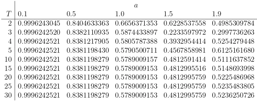
Table 1: Modulus of the transmission coefficient T for the case where σ = 0.2, k2 = 1.5,

h= 2.0, and θ= 0.25. Modes with|m|≤T and |n|≤T are retained in the field expansions.

All computations have been checked against the energy balance (4.18) and the errors caused by truncation and quadrature always amount to much less than 1% in the total energy. In each of the figures presented below, the value of T used in the calculations is stated and we have verified the results by computing them using a larger truncation value.

To reduce the number of parameters we have fixed σ = 0.2 throughout, which is a value representative of many rocks [26]. Our computations suggest that results are not particularly sensitive to the value of σ, which only enters the equations directly via (2.4). Note that σ = 0.2 corresponds to Λ = 3/8. To illustrate the convergence of our approach as T increases we present computed values of the modulus of the transmission coefficient T in Table 1. The two parameters which most significantly affect the convergence are the frequency and the gap between the cavity and the free surface. The frequency parameter used in the table is k2 = 1.5 which is neither a low frequency (where the multipole method

converges very quickly) or high frequency (where very little happens physically because the Rayleigh wave does not feel the presence of the cavity and passes over essentially unchanged). The cavity depth is h = 2 and we show results for five different cavity radii, ranging from 0.1 to 1.9, at which point the gap between the cavity and the free surface is small and we would expect the convergence to be less good. This is borne out by the numbers in the table, which show that the convergence improves as the gap between the cavity and the free surface increases. The table also demonstrates that except when the gap between the cavity and the free surface is small, we can expect to achieve very accurate results with moderate truncation sizes.

For normal incidence, Gregory [5] states a result for the reflection coefficient in the long-wave limit, by which we mean the limit a → 0 for fixed frequency, in which case the submergence remains O(1). Our numerical results do not fit with Gregory’s expression, nor do our attempts to reproduce it analytically. We have calculated the leading-order behaviour of the unknowns ξn(i) in this limit and find, in agreement with Gregory, that ξ₀(1), ξ_±(i)₁, ξ_±(i)₂, i = 1,2, are O(a2_{) whereas all the other coefficients (including ξ}(2)

0 ) are O(a4). However

when we insert the leading order contributions to ξn(i) into the formula for R, the result

expression agrees with our numerical results in this limit. We find that, to leading order,

ξ(1)0 ∼

iπa2

4

!

k₂2−k2₁"Ainc₀ ,

ξ_±(1)₁ ∼ πk1a 2

8

!

−ik1Ainc_±1∓k2B_±inc₁", ξ_±(2)₁ ∼ πk2a 2

8

!

±k1Ainc_±1−ik2B_±inc₁", (5.3)

ξ_±(1)₂ ∼ πk 2 1a2

4(k2 2−k12)

!

ik2₁Ainc_±2 ±k2₂B_±inc₂", ξ_±(2)₂ ∼ πk 2 2a2

4(k2 2 −k21)

!

∓k₁2Ainc_±2+ ik₂2B_±inc₂".

We now present figures showing the proportion of the total scattered energy due to the longitudinal P-waves (the contribution to (4.18) from M), the shear S-waves (the contri-bution to (4.18) from N and L) and the reflected and transmitted Rayleigh waves (the contributions to (4.18) fromR and T, respectively.

Figures 1 and 2 show results for a = 1, σ = 0.2, against frequency, for three different values of θinc. Figure 1 is a case of a relatively deep cavity (h = 2) whereas in Figure 2 the cavity is much closer to the surface (h = 1.3). At low frequency we have long waves which are largely unaffected by the relatively small cavity and we find that |T | → 1 as k2a → 0. At high frequency, the incident wave is tightly localised at the surface and we again find that |T | approaches 1 as k2a increases. At head on incidence, there isn’t much reflection and the contribution from the longitudinal P-wave is small. There is, however, a large range of frequencies for which the proportion of the incident wave energy that is converted into the S-wave is significant with a small range where this proportion is greater than 50%. For oblique incidence the picture becomes more complicated. For θinc = π/4 the picture is qualitatively the same as for head-on incidence but now there is no P-wave as this cuts offat

θinc = arcsin(k1/kR)≈0.188πand the amount of energy going into the S-wave now peaks at

over 75%. Forθinc = 0.35π we see much stronger effects at the higher frequencies with large spikes in the S-wave energy around k2a≈8.5 andk2a≈10.5. Note that the S-wave cuts off at θinc = arcsin(k2/kR) ≈ 0.365π. We can generate more interaction by moving the cavity closer to the surface and this is illustrated in Figure 2. There is now a much greater range of frequencies over which the incident wave energy is converted in significant proportions into reflected Rayleigh and scattered bulk waves.

Figures 3 and 4 show results for a = 1, σ = 0.2, against angle of incidence, for three different values of k2a. Figure 3 is a case of a relatively deep cavity (h = 2) whereas in Figure 4 the cavity is much closer to the surface (h = 1.3). The figures show the sharp (but continuous) cut off of the circular waves at θinc ≈ 0.188π and θinc ≈ 0.365π. As θ

increases, |T | starts to develop oscillations. Initially these are matched by oscillations in the contribution from the shear circular wave, but after this switches off there are strong oscillations in |R|. These oscillations correspond to the region in which modes propagate along the surface of a cylindrical cavity in the absence of a free surface [22]. Calculations show that the spikes in the figures do not correspond precisely to the values of ℓ at which the modes occur, but in all cases there are a number of modes which occur for ℓ > k2, i.e.

(a)

0 4

0.00 0.25 0.50 0.75 1.00

k2

8 12 16

(b)

0 4

0.00 0.25 0.50 0.75 1.00

k2

8 12 16

(c)

P S |R|2 _{|T |}2

0 4

0.00 0.25 0.50 0.75 1.00

k2

8 12 16

(a)

0 4

0.00 0.25 0.50 0.75 1.00

k2

8 12 16

(b)

0 4

0.00 0.25 0.50 0.75 1.00

k2

8 12 16

(c)

P S |R|2 _{|T |}2

0 4

0.00 0.25 0.50 0.75 1.00

k2

8 12 16

(a)

θinc

0 π/4 π/2

0.00 0.25 0.50 0.75 1.00

(b)

θinc

0 π/4 π/2

0.00 0.25 0.50 0.75 1.00

(c)

θinc

P S |R|2 _{|T |}2

0 π/4 π/2

0.00 0.25 0.50 0.75 1.00

Figure 3: Proportion of scattered energy associated with P-, S-, reflected and transmitted waves whena_{= 1,} h_{= 2,}σ_{= 0}._{2, as a function of}θinc, with (a)k2a=π, (b)k2a= 2π, (c)k2a= 3π, computed with truncation parametersT _{= 8, 10 and 12, respectively. The solid squares identify the critical angles} θ∗

1 ≈0.188π and

θ∗

(a)

θinc

0 π/4 π/2

0.00 0.25 0.50 0.75 1.00

(b)

θinc

0 π/4 π/2

0.00 0.25 0.50 0.75 1.00

(c)

θinc

P S |R|2 _{|T |}2

0 π/4 π/2

0.00 0.25 0.50 0.75 1.00

Figure 4: Proportion of scattered energy associated with P-, S-, reflected and transmitted waves when

a _{= 1,} h _{= 1}._3, σ _{= 0}._{2, as a function of} θinc, with (a) k2a =π, (b) k2a = 2π, (c) k2a = 3π, computed with truncation parameters T _{= 8, 10 and 12, respectively. The solid squares identify the critical angles}

θ∗

A

Mutipoles

The aim is to construct solutions to Navier’s equation (2.1) which are (i) of the form u = ˜

u(x, z)eiℓy_{, (ii) singular atz =−h(h >0), (iii) satisfy the condition of zero traction onz = 0}

and (iv) represent outgoing waves as |x| → ∞. Singular solutions of the two-dimensional Helmholtz equation (∇2_+k2_{)u= 0 are given by}

Hn(kr)einθ =

1

πi

1 ∞

−∞

e−kγ(t)|z+h|eikxt(t−γ(t))nsgn(z+h) dt

γ(t), (A.1)

where γ(z) = (z2 ₋₁₎1/2 _{with branch cuts along along (1,1 + i∞) and (−1,−1−i∞) and}

the path of integration is indented so as to pass above the branch point att =−1 and below that at t = 1 (see, for example, [27], but note that here rsinθ = x, rcosθ = −(z+h)). If we make the substitution kt=s we obtain

Hn(kr)einθ =

1

πiknsgn(z+h)

1 ∞

−∞

e−˜γ(s;k)|z+h|eisx(s−γ˜(s;k))nsgn(z+h) ds ˜

γ(s;k), (A.2)

where ˜γ(s;k) = (s2_−k2₎1/2_{. This form is valid for non-zero complexk with the branch cuts}

as described above, provided Re ˜γ > 0 as |s| → ∞. In particular, it is valid for k = iq,

q >0, and we note that in this case the Hankel function becomes a modified Bessel function: Hn(iqr) = (2/πin+1) Kn(qr).

Provided κ1 ̸= 0, multipoles ˜u(i)n are triples {φ(i)n ,ψ(i)n ,χ(i)n }, i= 1,2,3 of the form

φ(1)_n = Hn(κ1r)einθ+

1

πiκn 1

1 ∞

−∞

A(1)eγ1(z−h)_eisx_(s−γ

1)n

ds

γ1, (A.3)

= 1

πiκn 1

1 ∞

−∞

-e−γ1(z+h)_+A(1)_eγ1(z−h)._eisx_(s−γ1)nds

γ1, z >−h, (A.4)

ψ(1)_n = 1

πiκn 1

1 ∞

−∞

B(1)e−γ1h_eγ2z_eisx_(s−_γ1)n_{ds, (A.5)}

χ(1)_n = 1

πiκn 1

1 ∞

−∞

C(1)e−γ1h_eγ2z_eisx_(s−γ1)n_{ds, (A.6)}

and provided κ2 ̸= 0 we have

φ(2)_n = 1

πiκn 2

1 ∞

−∞

A(2)e−γ2h_eγ1z_eisx_(s−γ2)n_{ds, (A.7)}

ψ_n(2) = Hn(κ2r)einθ+

1

πiκn 2

1 ∞

−∞

B(2)eγ2(z−h)_eisx_(s−γ

2)n

ds

γ2, (A.8)

= 1

πiκn 2

1 ∞

−∞

-e−γ2(z+h)_+B(2)_eγ2(z−h)._eisx_(s−γ2)nds

γ2, z >−h, (A.9)

χ(2)_n = 1

πiκn 2

1 ∞

−∞

and

φ(3) n =

1

πiκn 2

1 ∞

−∞

A(3)_e−γ2h_eγ1z_eisx_(s−γ

2)nds, (A.11)

ψ(3)_n = 1

πiκn 2

1 ∞

−∞

B(3)eγ2(z−h)_eisx_(s−γ2)n_{ds, (A.12)}

χ(3)_n = Hn(κ2r)einθ+

1

πiκn 2

1 ∞

−∞

C(3)eγ2(z−h)_eisx_(s−_γ2)nds

γ2, (A.13)

= 1

πiκn 2

1 ∞

−∞

-e−γ2(z+h)_+C(3)_eγ2(z−h)._eisx_(s−γ2)nds

γ2

, z >−h, (A.14)

whereγi = ˜γ(s;κi) = (s2−κ2i)1/2 =−i(κ2i−s2)1/2. The precise interpretation of the contours

will be determined once the functions A(i)_{, B}(i) _{and C}(i) _{have been formally determined.}

For the multipole triple {φ(1)n ,ψn(1),χ(1)n }, application of the boundary conditions (2.19),

(2.21) and (2.22) yields

A(1) =−1

∆((2ˆs

2_−k2

2)2+ 4ˆs2γ1γ2) =−1−

8ˆs2_γ1γ2

∆ ,

B(1) =−4isk 2 2 κ2

2∆

(2ˆs2−k₂2), C(1) = 4ik2γ2ℓ

κ2 2∆

(2ˆs2−k2₂),

(A.15)

where we have written ˆs2 _=s2_+ℓ2 _and

∆= (2ˆs2−k2₂)2−4ˆs2γ1γ2 = (2s2−ν2)2−4ˆs2γ1γ2. (A.16)

Note that A(1)_{(s) and C}(1)_{(s) are even functions, whereas B}(1)_{(s) is an odd function. Since} γ2

i = ˆs2−ki2, ∆is the secular determinant for Rayleigh waves with ∆= 0 implying

(2ˆs2 −k2₂)4 = 16ˆs4(ˆs2−k2₁)(ˆs2−k2₂), (A.17)

which simplifies to the cubic

(k₂2/sˆ2)3 −8(k₂2/sˆ2)2+ 8(k₂2/sˆ2)(3−2Λ)−16(1−Λ) = 0. (A.18)

Only the real root (for k2

2/ˆs2) lying in (0,1) is actually a solution to ∆ = 0 (the others,

when they exist, correspond to taking different branches in the definition of γi). This leads to poles in the integrands at ˆs2 _=k2

R or equivalently at s=±(kR2 −ℓ2)1/2 =±α. We choose

the contour of integration to be indented above the pole ats=−αand below that at s=α. This will ensure that the multipole behaves like an outgoing wave as |x|→ ∞.

Similarly for the multipole triple {φ(2)n ,ψ(2)n ,χ(2)n }

A(2) = 4is ∆(2ˆs

2_−k2

2), B(2) =−1−

8γ1γ2k2 2s2 κ2

2∆

, C(2) = 8γ1γ2ℓsk2

κ2 2∆

. (A.19)

Note thatA(2)_{(s) andC}(2)_{(s) are odd functions, whereasB}(2)_{(s) is an even function. Finally,}

for the triple {φ(3)n ,ψn(3),χ(3)n } we have

A(3) =−4iγ2ℓ k2∆(2ˆs

2_−k2

2), B(3) =C(2), C(3) = 1−

8γ1γ3 2ℓ2 κ2

2∆

Note thatA(3)_{(s) and C}(3)_{(s) are even functions, whereasB}(3)_{(s) is an odd function.}

Polar expansions of the multipoles can be obtained as follows: define ui according to

s=κicoshui, γi =κisinhui, i.e.,

eui _{= (s+γ}

i)/κi, e−ui = (s−γi)/κi. (A.21)

In other words, if κi = iqi,qi >0, then

ui =−πi

2 + sinh

−1 s

qi. (A.22)

On the other hand, if κi >0 is real, then

ui = ⎧ ⎪ ⎨ ⎪ ⎩

−iπ−cosh−1|_κs|

i, s < −κi,

−i cos−1 s

κi, −κi < s <κi,

cosh−1 _κs

i, s >κi.

(A.23)

In all cases we have ui(−s) =−iπ−ui(s). Then, as in (3.14),

eγiz_eisx _{= e}−γih

∞

%

n=−∞

Jn(κir)einθe−nui. (A.24)

Hence

φ(1)

n = Hn(κ1r)einθ+ ∞

%

m=−∞ A(1)

nmJm(κ1r)eimθ,

ψ_n(1) =

∞

%

m=−∞

B(1)_nmJm(κ2r)eimθ, χ(1)n = ∞

%

m=−∞

C_nm(1)Jm(κ2r)eimθ,

(A.25) where A(1) nm = 1 πi 1 ∞ −∞

A(1)_e−2γ1h_e−(m+n)u1ds

γ1,

B_nm(1) = 1

πi

1 ∞

−∞

B(1)e−(γ1+γ2)h_e−mu2−nu1_{ds, C}(1)

nm=

1

πi

1 ∞

−∞

C(1)e−(γ1+γ2)h_e−mu2−nu1_ds. (A.26) For the multipole triple{φ(2)n ,ψn(2),χ(2)n }we have

φ(2) n = ∞ % m=−∞ A(2)

nmJm(κ1r)eimθ, χ(2)n = ∞

%

m=−∞ C(2)

nmJm(κ2r)eimθ,

ψ(2)

n = Hn(κ2r)einθ+ ∞

%

m=−∞ B(2)

nmJm(κ2r)eimθ,

(A.27)

where

A(2)_nm = 1

πi

1 ∞

−∞

A(2)e−(γ1+γ2)h_e−mu1−nu2_{ds, C}(2)

nm =

1

πi

1 ∞

−∞

C(2)e−2γ2h_e−(m+n)u2_ds,

B(2) nm = 1 πi 1 ∞ −∞

B(2)_e−2γ2h_e−(m+n)u2ds

γ2,

and for the triple {φ(3)n ,ψ(3)n ,χ(3)n },

φ(3)_n =

∞

%

m=−∞

A(3)_nmJm(κ1r)eimθ, ψn(3) = ∞

%

m=−∞

B_nm(3) Jm(κ2r)eimθ,

χ(3)_n = Hn(κ2r)einθ+ ∞

%

m=−∞

C_nm(3)Jm(κ2r)eimθ,

(A.29)

where

A(3)_nm= 1

πi

1 ∞

−∞

A(3)e−(γ1+γ2)h_e−mu1−nu2_{ds, B}(3)

nm=Cnm(2),

C_nm(3) = 1

πi

1 ∞

−∞

C(3)e−2γ2h_e−(m+n)u2ds

γ2.

(A.30)

Note that changing s to −s shows that

A(i)_nm = (−1)n+m+i+1A−n,−m(i) , Bnm(i) = (−1)n+m+iB (i)

−n,−m, Cnm(i) = (−1)n+m+i+1C (i) −n,−m.

(A.31)

Far field

We wish to determine the asymptotic behaviour of the multipoles as R → ∞, uniformly in Θ, whereRandΘare polar coordinates centred at the origin, i.e.x=RsinΘ,z =−RcosΘ. Note that

r=R−hcosΘ+O(R−1), θ =Θ+O(R−1). (A.32)

We have, from (A.3) and (A.15),

φ(1)_n = Hn(κ1r)einθ−

1

πiκn 1

1 ∞

−∞

#

1 + 8ˆs

2_γ1γ2

∆(s)

$

eγ1(z−h)_eisx_(s−γ1)nds

γ1

, (A.33)

= Hn(κ1r)einθ−

1

πi

1 ∞

−∞

#

1 + 8κ1(κ

2

1t2+ℓ2)γ2(κ1t)γ

∆(κ1t)

$

e−2κ1hγ_eκ1rg(t)_(t−γ)ndt

γ ,

(A.34)

where

g(t) =−γ(t) cosθ+ itsinθ. (A.35)

The asymptotics as R → ∞ can readily be determined as shown in detail for the case of normal incidence in [4]. The leading order behaviour comes from two contributions: from the poles on the real axis (which are most easily calculated from (A.33)) and from the saddle point corresponding to the root of g′_{(t) = 0 (which can be deduced from (A.34)). In fact}

φ(1)_n ∼M_n(1)±e±iαxeβ1z_+M(1)

n (Θ)

,

2

πκ1R e

i(κ1R−π/4)_+O(R−1_{), (A.36)}

where the upper sign is to be taken ifx >0 and the lower sign ifx <0. Ifκ2

1 <0, the saddle

point contribution is exponentially small.

To determine Mn(1)± we note that the poles are at s=±α, at which points

ˆ

We define

∆′ ₌ d∆

ds

7 7 7

s=α=−

d∆ ds

7 7 7

s=−α=

4α

β1β2(β2−β1)

!

k2

R(β1 −β2) + 2β1β22

"

(A.38)

and note that this cannot vanish since β1 > β2 > 0. When x > 0 the contributing pole is at s=α, whereas when x <0 it is the pole at s=−α that contributes. Thus, from (A.33) and (3.11),

M_n(1)± =−16k 2 Rβ2

∆′ e −β1h

#

±α−β1 κ1

$n

=−(±1)n16kR2β2

∆′ e

−β1h_e∓nζ1_{. (A.39)}

To determine M(1)n (Θ) we first note that g′(t) = 0 if and only if t =t∗ = sinθ and that

γ(t∗) = −i cosθ, g(t∗) = i, g′′(t∗) = −i/cos2θ. (A.40)

The two steepest descent contours from the saddle point make angles −π/4 and 3π/4 with the positivex-axis and hence if we deform the contour of integration into the path of steepest descent we can then calculate the contribution from the saddle point using the expression [28, eqn. 7.2.10]

f(t∗)eκ1rg(t∗)_e−iπ/4

8

2π κ1r|g′′_(t∗_)|.

There is also a contribution from the Hankel function. Thus, from (A.34) using (A.32),

M(1)

n (Θ) = (−i)ne−iκ1hcosΘeinΘ+

#

8κ1G1(κ12sin2Θ+ℓ2) cosΘ

∆(κ1sinΘ) −1

$

ineiκ1hcosΘ_e−inΘ_, (A.41) where

G1 = iγ2(κ1sinΘ) = i(κ21sin2Θ−κ22)1/2 = (κ22−κ21sin2Θ)1/2. (A.42)

For φ(2)n we have, from (A.7) and (A.19),

φ(2)n =

4

πκn 2

1 ∞

−∞ s

∆(2ˆs

2_−k2

2)e−γ2heγ1zeisx(s−γ2)nds (A.43)

= 4κ1

πκn 2

1 ∞

−∞ κ1t

∆(κ1t)(2κ

2

1t2−ν2)e−(κ1γ+γ2(κ1t))heκ1rg(t)(κ1t−γ2(κ1t))ndt (A.44)

and hence

φ(2)_n ∼M_n(2)±e±iαxeβ1z₊M(2)

n (Θ)

,

2

πκ1R e

i(κ1R−π/4)_+O(R−1_{), (A.45)}

with

M(2)±

n = (±1)n+1

8iα

∆′ (k 2

R+β22)e−β2he∓nζ2 (A.46)

and

M(2)_n (Θ) = 4κ

2

1sinΘcosΘ

∆(κ1sinΘ) (2κ

2

1sin2Θ−ν2)eiG1h

#

κ1sinΘ+ iG1 κ2

$n

. (A.47)

If κ2

For φ(3)n we have, from (A.11) and (A.20),

φ(3)_n =− 4ℓ πκn

2

1 ∞

−∞ γ2 k2∆(2ˆs

2_−k2

2)e−γ2heγ1zeisx(s−γ2)nds (A.48)

=−4ℓκ1 πκn 2

1 ∞

−∞

γ2(κ1t)

k2∆(κ1t)(2κ

2

1t2−ν2)e−(κ1γ+γ2(κ1t))heκ1rg(t)(κ1t−γ2(κ1t))ndt (A.49)

and hence

φ(3)

n ∼Mn(3)±e±iαxeβ1z+M(3)n (Θ)

,

2

πκ1R e

i(κ1R−π/4)_+O(R−1_{), (A.50)}

with

M_n(3)± =−(±1)n8iβ2ℓ k2∆′(k

2

R+β22)e−β2he∓nζ2 (A.51)

and

M(3)_n (Θ) = 4iℓκ1G1cosΘ

k2∆(κ1sinΘ)

(2κ2₁sin2Θ−ν2)eiG1h

#

κ1sinΘ+ iG1 κ2

$n

. (A.52)

If κ2

1 <0, the saddle point contribution is exponentially small.

Forψ(i)n and χ(i)n there is an additional complication due to the fact that the saddle point

at s = κ2sinθ can coincide with the branch point at s = κ1. However, as shown in [4] the

only consequence of this is that the error term becomes O(R−3/4_{) rather thanO(R}−1_{). Thus}

for ψn(1) we have, from (A.5) and (A.15),

ψ(1)n =−

4k2 2 πκ2

2κn1

1 ∞

−∞ s

∆(2ˆs

2₋

k22)e−γ1heγ2zeisx(s−γ1)nds (A.53)

=−4k 2 2 πκn 1 1 ∞ −∞ t(2κ2

2t2−ν2)

∆(κ2t)

e−(κ2γ+γ1(κ2t))h_eκ2rg(t)_{(κ2t−γ1(κ2t))}n_{dt (A.54)}

and hence

ψ(1)_n ∼N_n(1)±e±iαxeβ2z_+N(1)

n (Θ)

,

2

πκ2R

ei(κ2R−π/4)_+O(R−3/4_{), (A.55)}

with

N(1)±

n =−(±1)n+1

8iαk2 2 κ2

2∆′

(k2

R+β22)e−β1he∓nζ1 (A.56)

and

N_n(1)(Θ) = 4k

2

2sinΘcosΘ(ν2 −2κ22sin2Θ)

∆(κ2sinΘ) e

iG2h

#

κ2sinΘ+ iG2 κ1

$n

, (A.57)

where

G2 = iγ1(κ2sinΘ) = i(κ22sin2Θ−κ12)1/2 = (κ21−κ22sin2Θ)1/2. (A.58)

For ψn(2) we have, from (A.8) and (A.19),

ψ_n(2) = Hn(κ2r)einθ−

1

πiκn 2

1 ∞

−∞

#

1 + 8γ1γ2k

2 2s2 κ2

2∆

$

eγ2(z−h)_eisx_(s−γ2)nds

γ2 (A.59)

= Hn(κ2r)einθ−

1

πi

1 ∞

−∞

#

1 + 8γ1(κ2t)γκ2k

2 2t2

∆

$

e−2κ2hγ_eκ2rg(t)_(t−γ)ndt

and so

ψ(2)_n ∼N_n(2)±e±iαxeβ2z _+N(2)

n (Θ)

,

2

πκ2R

ei(κ2R−π/4)_+O(R−3/4_{), (A.61)}

with

N_n(2)± =−(±1)n16β1k

2 2α2 κ2

2∆′

e−β2h_e∓nζ2 _(A.62)

and

N(2)

n (Θ) = (−i)ne−iκ2hcosΘeinΘ+

#

8G2κ2k2

2sin2ΘcosΘ

∆(κ2sinΘ) −1

$

ineiκ2hcosΘ_e−inΘ_{. (A.63)}

For ψn(3) we have, from (A.12) and (A.20),

ψ(3)_n = 8ℓk2

πiκn+2 2

1 ∞

−∞ γ1γ2s

∆ e

γ2(z−h)_eisx_(s−γ

2)nds (A.64)

= 8ℓk2κ2

πi

1 ∞

−∞

γ1(κ2t)γt

∆(κ2t) e

−2κ2γh_eκ2rg(t)_(t−γ)n_{dt (A.65)}

and so

ψ(3)_n ∼N_n(3)±e±iαxeβ2z _+N(3)

n (Θ)

,

2

πκ2R e

i(κ2R−π/4)_+O(R−3/4_{), (A.66)}

with

N_n(3)± = (±1)n+116ℓk2β1β2α

κ2 2∆′

e−β2h_e∓nζ2 _(A.67)

and

N(3)

n (Θ) =

8iℓk2κ2G2sinΘcos2Θ

∆(κ2sinΘ) i

n_eiκ2hcosΘ_e−inΘ_{. (A.68)}

In a similar way we can show that

χ(i)_n ∼L(i)_n ±e±iαxeβ2z_+L(i)

n (Θ)

,

2

πκ2R e

i(κ2R−π/4)_+O(R−3/4_{), (A.69)}

with

L(1)_n ± = (±1)n8ik2ℓβ2 κ2

2∆′

(k_R2 +β₂2)e−β1h_e∓nζ1_{, (A.70)}

L(2)_n ± = (±1)n+116ℓk2β1β2α

κ2 2∆′

e−β2h_e∓nζ2_{, L}(3)±

n =L(2)n ± ℓβ2

k2α, (A.71)

and

L(1)_n (Θ) =−4ik2ℓcos 2_Θ

∆(κ2sinΘ)(2κ

2

2sin2Θ−ν2)eiG2h

#

κ2sinΘ+ iG2 κ1

$n

, (A.72)

L(2) n (Θ) =

8iℓk2κ2G2sinΘcos2Θ

∆(κ2sinΘ) i

n_eiκ2hcosΘ_e−inΘ_{, (A.73)}

L(3)

n (Θ) = (−i)ne−iκ2hcosΘeinΘ+

#

1− 8κ2G2ℓ

2_cos3_Θ

∆(κ2sinΘ)

$

ineiκ2hcosΘ_e−inΘ_{. (A.74)}

If κ2

2 <0, the saddle point contributions in ψ (i)

The limits

κ

→

0

and

κ

→

0

Many equations in this paper include terms that do not exist in the limitsκ1 →0 andκ2 →0. To show that our method remains valid in these cases, we introduce scaled coefficients into (3.16), via

ξ_n(1) =κ|₁n|ξ˜_n(1), and ξ_n(j)=κ|₂n|ξ˜_n(j), j = 2,3. (A.75) To verify that these scalings are correct, we must show that all singularities in the far field and in the coefficients of the linear system formed from (3.26)–(3.28) are now removable. The definitions of the functionsA(j)_,B(j) _{and C}(j) _{remain valid as κ1 →0, but the function} γ1 appears in the denominator in (A.3) and this could potentially introduce a singularity that is not removable. However, using (A.15), we can write

φ(1)_n = Hn(κ1r)einθ−Hn(κ1r˜)ein ˜

θ₋ 8

πiκn 1

1 ∞

−∞

ˆ

s2_γ2

∆ e

−γ1(h−z)_eisx_(s−_γ1)n_{ds, (A.76)}

where the polar coordinate system (˜r,θ˜) is centred at the point (0, h), so that ˜rsin ˜θ = x

and ˜rcos ˜θ =h−z. Evidently the integral in (A.76) remains bounded in the limit κ1 →0,

if n ≥0. If n < 0, we rewrite it using the identity

s−γ1 κ1 =

κ1

s+γ1. (A.77)

We can then use [29, eqn. 10.7.7] to show that φ(1)n =O(κ1−|n|) if n̸= 0. On the other hand,

if n = 0 then the integral poses no problem, and we can take the limit κ1 → 0 using [29, eqn. 10.7.2].

With the coefficients scaled as in (A.75), the only potentially singular term in the linear system formed from (3.26)–(3.28) is

T =−ν¯2ξ₀(1)!H01+A(1)₀₀J01", (A.78)

from (3.26) with m = 0. However, using (A.15), we can write A(1)₀₀ from (A.26) with m =

n= 0 in the form

A(1)₀₀ =−H0(2κ1h)−

8

πi

1 ∞

−∞

ˆ

s2_γ2

∆ e

−2γ1h_{ds, (A.79)}

which shows that T is regular in the limit κ1 →0.

A similar procedure can be used for the limit κ2 →0, though in this case the breakdown of the Helmholtz decomposition mentioned after (3.9) introduces additional complications, and we do not reproduce the details here. Another example of a problem involving an infinite linear system of equations in which certain coefficients are singular, but where a nontrivial solution still exists, can be found in [30].

References

[1] F. Ursell. Surface waves on deep water in the presence of a submerged circular cylinder I. Proc. Camb. Phil. Soc., 46:141–152, 1950.

[3] W. E. Bolton and F. Ursell. The wave force on an infinitely long circular cylinder in an oblique sea. J. Fluid Mech., 57:241–256, 1973.

[4] R. D. Gregory. An expansion theorem applicable to problems of wave propagation in an elastic half-space containing a cavity. Proc. Camb. Phil. Soc., 63:1341–1367, 1967.

[5] R. D. Gregory. The propagation of waves in an elastic half-space containing a cylindrical cavity. Proc. Camb. Phil. Soc., 67:689–710, 1970.

[6] V. W. Lee and M. D. Trifunac. Response of tunnels to incident SH-waves. Journal of the Engineering Mechanics Division (ASCE), 105(4):643–659, 1979.

[7] Michael E. Manoogian and Vincent W. Lee. Diffraction of SH-waves by subsurface inclusions of arbitrary shape. J. Engrg. Mech., 122(2):123–129, 1996.

[8] C. Smerzini, J. Avil´es, R. Paolucci, and F. J. S´anchez-Sesma. Effect of underground cavities on surface earthquake ground motion under SH wave propagation. Earthquake Engineering and Structural Dynamics, 38:1441–1460, 2009.

[9] F. H¨ollinger and F. Ziegler. Scattering of pulsed Rayleigh surface waves by a cylindrical cavity. Wave Motion, 1:225–238, 1979.

[10] V. W. Lee and J. Karl. Diffraction of SV waves by underground, circular, cylindrical cavities. Soil Dynamics and Earthquake Engineering, 11:445–456, 1992.

[11] S. K. Datta and N. El-Akily. Diffraction of elastic waves by cylindrical cavity in a half-space. J. Acoust. Soc. Am., 64(6):1692–1699, 1978. Erratum: 65(5):p.1342, 1979.

[12] N. El-Akily and S. K. Datta. Response of a circular cylindrical shell to disturbances in a half-space. Earthquake Engineering and Structural Dynamics, 8:469–477, 1980.

[13] N. El-Akily and S. K. Datta. Response of a circular cylindrical shell to disturbances in a half-space—numerical results. Earthquake Engineering and Structural Dynamics, 9:477–487, 1981.

[14] C. C. Mei. Extensions of some identities in elastodynamics with rigid inclusions.

J. Acoust. Soc. Am., 64(5):1514–1522, 1978.

[15] J. N. Newman. Interaction of waves with two-dimensional obstacles: a relation between the radiation and scattering problems. J. Fluid Mech., 71:273–282, 1975.

[16] Fred L. Neerhoff. Reciprocity and power-flow theorems for the scattering of plane elastic waves in a half space. Wave Motion, 2(2):99–113, 1980.

[17] F. C. P. de Barros and J. E. Luco. Diffraction of obliquely incident waves by a cylindrical cavity embedded in a layered viscoelastic half-space. Soil Dynamics and Earthquake Engineering, 12(3):159–171, 1993.

[19] F. Ursell. Trapping modes in the theory of surface waves. Proc. Camb. Phil. Soc., 47:347–358, 1951.

[20] P. McIver and D. V. Evans. The trapping of surface waves above a submerged horizontal cylinder. J. Fluid Mech., 151:243–255, 1985.

[21] M. A. Biot. Propagation of elastic waves in a cylindrical bore containing a fluid.J. Appl. Phys., 23(9):997–1005, 1952.

[22] A. Bostr¨om and A. Burden. Propagation of elastic surface waves along a cylindrical cavity and their excitation by a point force. J. Acoust. Soc. Am., 72(3):998–1004, 1982.

[23] K. F. Graff. Wave Motion in Elastic Solids. Oxford University Press, 1975.

[24] G. N. Watson. A Treatise on the Theory of Bessel Functions. Cambridge University Press, 2nd edition, 1944.

[25] A. M. Turing. A method for the calculation of the zeta-function. Proceedings of the London Mathematical Society, 48(3):180–197, 1945.

[26] H. Fossen. Structural Geology. Cambridge University Press, 2010.

[27] C. M. Linton and D. V. Evans. The radiation and scattering of surface waves by a vertical circular cylinder in a channel. Phil. Trans. R. Soc. Lond., A, 338:325–357, 1992.

[28] Norman Bleistein and Richard A. Handelsman. Asymptotic Expansions of Integrals. Dover Publications, New York, 1986. Originally published in 1975.

[29] F. W. J. Olver, D. W. Lozier, R. F. Boisvert, and C. W. Clark, editors. NIST Handbook of Mathematical Functions. NIST and Cambridge University Press, 2010.