Advanced Line Sampling for Efficient Robust
Reliability Analysis
Marco de Angelis∗, Edoardo Patelli, Michael Beer Institute for Risk and Uncertainty, University of Liverpool
Liverpool, United Kingdom
Abstract
In this paper, a novel strategy is designed to efficiently estimate set-valued
failure probabilities, coupling Monte Carlo sampling-based with optimization methods. The notion of uncertainty is generalized to include both aleatory
and epistemic uncertainties, and capture gaps of knowledge and scarcity of
data. The proposed formulation of the generalized uncertainty model allows
for sets of probability distribution functions, also known as credal sets, and sets
of bounded variables. An Advanced Line Sampling method is developed and
combined with the generalized uncertainty model, not only to reduce the time
needed for a single reliability analysis, but also to increase the efficiency of the
search for lower and upper bounds of the failure probability. The proposed
strategy knocks down the computational barrier of computing interval failure
probabilities, and reduces the cost of a robust reliability analysis by many orders of magnitude. The solution strategy is integrated into the open-source software
for uncertainty quantification and risk analysis OpenCossan, allowing its
appli-cation on large-scale engineering problems as well as broadening its spectrum of
potential applications. The efficiency and applicability of the developed method
is demonstrated via numerical examples.
Keywords: Structural Reliability, Monte Carlo Methods, Line Sampling,
Credal Sets, Bounded Sets, Set-valued Probabilities, Generalized Uncertainty
∗Corresponding author
Model, Aleatory Uncertainty, Epistemic Uncertainty
1. Introduction
Engineering structures and systems, such as bridges, buildings, aircraft,
off-shore platforms, nuclear power plants, transmission towers and pipelines, are
designed to fulfil specific requirements, and they should be able to deal with
possible changes of loads and conditions. However, the design context is often 5
characterized by partial knowledge and limited access to information. In such a
context, in order to be able to bypass the difficulties in quantifying vague
infor-mation, decisions often rely on experts opinions, rather than rigorous analyses.
In this paper a generalized model of uncertainty is proposed and used for
relia-bility assessment to address this issue. Within this model the risk is evaluated 10
treating gaps of knowledge and scarcity of data as a key source of uncertainty.
To translate this into practice, computational models that consider imprecision
are proposed.
Risk is conventionally expressed as the product between the failure
proba-bility of the system and the consequences caused by the system’s failure. While 15
the consequences are quantified in monetary units, the failure probability is
cal-culated, within a reliability assessment, in a rigorous probabilistic framework
[1]. Commonly, this requires the specification of precise distributional models
(of probability), including dependencies for the input variables.
Among the numerical methods proposed to assess reliability, simulation 20
methods [2] have attracted significant attention. Simulation methods are
gener-ally applicable, but require a compromise between efficiency and accuracy.
Sim-ulation methods proposed in literature include Monte Carlo SimSim-ulation [3, 4],
Importance Sampling [5, 6], Directional Sampling [7, 8], Line Sampling [9, 10],
Subset Simulation [11] etc. The individual developments possess different per-25
formance features for different classes of problems. Herein, we target at high
numerical efficiency assuming that the limit state surfaces only show moderate
this does not impose a strong restriction. Hence, Line Sampling is selected as
the basis for our development, which has been extended to deal with generalized 30
probabilistic models.
The paper is organized as follows: In Section 2 a generalized uncertainty
model is introduced. In Section 3, an Advanced Line Sampling method and
adaptive algorithm is developed and, in Section 4, it is implemented in the
generalized uncertainty framework. In Section 5, the integration in the general 35
computational toolbox OpenCossan is briefly explained. In Section 6, numerical
examples are given to demonstrate the efficiency of the method. Final remarks
and conclusions are provided in Section 7.
2. A generalized uncertainty model
Traditionally, the assessment of structural reliability is based on well-defined 40
(precise) probabilistic models [1]. Probabilistic models are constructed from
data that, in a design context, are often scarce and not available to a sufficient
extent [13]. In such a context, it is advisable to relax the assumption of a precise
probabilistic model. A detailed reasoning and discussion in this direction with
an overview on available generalized models is provided in [14]. 45
In essence, a generalized model of uncertainty shall allow for imprecision in
both the state variables of the system, denoted asθ, and the parameters of the
probabilistic modelp. Depending on the amount of information available about
the variables and parameters, imprecision can be modelled in different ways,
for example by means of Intervals [15, 16, 17], Convex Models [18] and Fuzzy 50
Sets [19, 20]. Intervals are used when variables are only known to be bounded
within lower and upper limits, while Convex Models are used when variables are
known to be bounded and also show some dependences. Fuzzy Sets allow the
simultaneous analysis of different bounded sets, which is helpful if the bounds
are not known precisely and to explore sensitivity with respect to the bounds 55
of the inputs. When imprecision is also present within the probabilistic model,
This is the case, for example, when statistical distributions given along with
their confidence intervals are considered, or when data complying with several
statistical distribution models are processed. Credal Sets [21] provide a quite 60
general pathway to express and analyse sets of probability distributions. Thus,
we utilize credal sets in combination with bounded sets for the subsequent
de-velopment.
2.1. Credal sets and bounded sets
The generalized model of uncertainty, denoted byM, defines type and extent 65
of uncertainty in the state variablesθ. The model M may represent a credal
set C (see e.g. [21]), a bounded (interval) set Q (see e.g. [18]), or both at the
same time.
A credal set of category I, namely CI, is a set of probability distribution
functions, where the imprecision is defined in the distribution parameters. A 70
credal set of category II,CII, is a set of probability distribution functions, where
the imprecision is in the type of distribution functions (e.g. Normal, Log-normal,
Gamma, Beta), whilst a credal set of category III, CIII, has both imprecise
distribution parameters and function type.
A bounded set of category I, namelyQI, is obtained by the Cartesian prod-75
uct
×
bixi of interval variables xi = {xi |xi∈[xi, xi]⊂R}, i = 1, ..., b. Abounded set of category II, namelyQII, is obtained from interval variablesxi,
taking into account dependencies between the variables. This may be done in
many different ways, for example using convex sets, i.e. by constructing the
enclosing ellipsoid (see e.g. [22]), or using other types of sets (e.g. convex hulls, 80
polytopes).
In this paper, without limiting generality but providing a basic development,
only uncertainties where the imprecision is of category I are considered, thus
the setsCI andQI will be simply denoted as CandQ respectively.
2.2. Problem formulation
85
In performance-based engineering the structural system is considered as a
the state variables θ ∈ Θ⊆ Rn (see e.g. [23]). Typically, the state variables
are the inputs that defines the structural system, such as material properties,
shape and size of structural elements, and load magnitudes, whilst the perfor-90
mances express specific structural responses, such as frequency and amplitude
of vibrations, stresses, deflections and so forth.
The performance function g : Rn → g
i ∈ R maps values from the state
space Θ to the performance variables of interest. For given criteria on the
performance variables,g defines the failure domain ΘF ={θ∈Θ|g(θ)≤0}, 95
which is identified by the limit state surface ˜Θ ={θ |g(θ) = 0}. Points ˜θ on
the limit state surface are referred to as limit state points. An important feature
for our development is that the limit state is invariant to the uncertainty model
M, because it is intrinsic in the structural system, i.e. depends solely on the
performance functiong. The uncertainty model only determines the probability 100
over the state space, but does not influence location of limit state points ˜θ.
In our study, M is represented by both credal sets and bounded sets of
category I. In the credal setC, imprecision is considered in the distribution
pa-rameters ofn1imprecise random variables, which is expressed with the bounded
setQ1of distribution parameters. A second bounded setQ2is used to describe 105
imprecision in the structural parameters, which are not associated with any
distribution model.
The state variables are, thus, split into n1 imprecise random variables ξ∈
Ω⊆Rn1belonging toCandn
2interval variablesx∈X ∈Rn2 belonging toQ2,
wheren1+n2=n. The credal set is defined asC={hD(ξ;p) |p∈Rm, p∈ Q1},
110
whereQ1is the bounded setQ1=
×
mi [pi, pi], hD is the joint probabilitydis-tribution function of random variables ξ, D is the distributional model, and
p are the distributional parameters. The bounded set of the remaining state
variables is expressed as the Cartesian productQ2=
×
n2
i [xi, xi].
2.3. Failure probability for generalized uncertainty
115
When the uncertainty model comprises only precisely defined probability
structural reliability is assessed in terms of a precise failure probability. Precise
measures of failure probability are obtained asp(ΘF,D,p) =RΘ
FhD(ξ;p)dΘ,
wheredΘ is the Lebesgue measure of an elementary portion of Θ. For simplic-120
ityp(ΘF,D,p) is subsequently denoted bypF. Operating with the generalized
uncertainty model M leads to imprecise measures of failure probability. The
failure domain is split into two separate domains as ΘF = ΩF ×XF, where
ΩF(x) = {ξ∈Rn1 |g(ξ,x)≤0} and XF(ξ) ={x∈Rn2 |g(ξ,x)≤0}.
Pro-vided the definition ofC, the imprecise failure probability is expressed as the 125
interval p
F(C,Q2) =
h
p
F(C,Q2), pF(C,Q2)
i
. The lower and upper bound of
the imprecise failure probability are
pF(C,Q2) = inf
x∈Q2
inf
p∈Q1 Z
ΩF(x)
hD(ξ;p)dΩ; pF(C,Q2) = sup
x∈Q2
sup
p∈Q1 Z
ΩF(x)
hD(ξ;p)dΩ,
(1) where, the order to which the operations of infimum and supremum are
per-formed can be changed. The inner operand searches the bounds of pF within
C, while the outer one searches the bounds ofpF withinQ2.
130
Upper and lower bounds of failure and survival probabilities show a dual
relationship. This can be seen clearly in the special case that the uncertainty
model is restricted toConly. The probability functionh◦D that yields the lower
boundp(ΩF), satisfies the equationR ΩFh
◦
D(ξ)dΩ+ R
ΩSh ◦
D(ξ)dΩ = 1, where ΩS
denotes the survival domain (complementary to the failure domain). Therefore, 135
h◦ is also the function for which the upper bound p(ΩS) is obtained. Thus,
the Equationp(ΩF) = 1−p(ΩS) establishes a dual (or conjugate) relationship between lower and upper probability functions. This relationship allows to
identify the upper probability function when the lower probability function is
known and vice versa. Note, however, that the complete function, which may 140
also have an infinite support, is needed in order for the relationship to be used.
From the definition of lower and upper probability follows thatp
F ≤pF. When
C degenerates into a single probability distribution function, precise measures
3. Advanced Line Sampling 145
The computation of failure probabilities can be associated with quite a
sig-nificant numerical effort. In cases where the number of random variables is high
and the limit state surface is nonlinear, methods based on the computation of
the Hessian become impractical. In these cases, advanced simulation methods,
represent a useful alternative. Here, a new method that extends the concept 150
of Line Sampling is presented. The method, named Advanced Line Sampling
(ALS), does not only increase the efficiency of single reliability analysis but it proves to be essential for finding the lower and upper bound of the failure
probability.
3.1. Concept of Line Sampling
155
Line Sampling, introduced in [9], and recently applied in [24], is an advanced simulation method developed to efficiently compute small failure probabilities
for high dimensional problems. The method requires the knowledge of the
so-called “important direction”,α∈Rn, which is defined as pointing towards the failure region. An initial approximation for the important direction is commonly
obtained by computing the gradient of the performance function in the origin
of the Standard Normal Space (SNS). Simulation methods estimate the failure
probability by computing the integral
pF =
Z ∞
−∞
IF(u)hN(u)du, (2)
where,IF :Rn → {0,1}is the indicator function,u=T(θ) are standard normal
variables, T : Rn →
Rn maps variablesξ from the original space to the SNS,
andhN(u) =Qni=1φ(ui) is the standard normal PDF. Provided that hN(u) is
invariant to rotation of the coordinate axes, Equation 2 can be written in the
form
pF =
Z ∞
−∞
Z ∞
−∞
IF(u)φ(u1)du1
n
Y
i=2
φ(ui)dui (3)
for convenient evaluations. Withu1 pointing orthogonally towards the failure
domain, the expansionw(u2:n) = R ∞
function of the n−1 remaining standard variables u2:n ∈ Rn−1 and provides
a measure of likelihood for the variableu2:n to be in the failure domain. All
of the points with coordinatesu⊥={0,u2:n}lie on the hyperplane orthogonal 160
to the first coordinateu1. Variable w can be calculated as w(u2:n) = Ψ(F1),
where Ψ(A) =R∞
−∞IA(y)φ(y)dy is the Gaussian measure of a subset ofA⊂R.
Let the scalar c∗ be the smallest (in magnitude) value of the coordinate u1
where the functionIF(u) steps from zero to one. This enableswto be
approxi-mately calculated asw(u2:n) = Φ(−|c∗|), where Φ is the standard normal CDF.
165
Therefore, the failure probability can be obtained as the expected value
pF =E[w(u2:n)] =
Z ∞
−∞
w(u2:n)
n
Y
i=2
φ(ui)dui. (4)
Note that considering the standard normal CDF Φ(−|c∗|) in place of the
Gaussian measure Ψ(F1), the probabilitywcan only be overestimated, because
it assumes that no further failure regions can be found on the line beyond
c∗. LS provides an estimation of E[w] by repeatedly generating points u2:n
from the standard normal PDF inRn−1, and computing the respective partial
probabilitiesw(u2:n). For example, generatingNL pointsu{ j}
2:n, j= 1,2, .., NL, an estimate of the failure probability is obtained computing the average
ˆ pF =
1 NL
NL X
j
w(u{2:jn}). (5)
Despite the important directionαis not oriented as the first coordinateu1,
the above integrals can still be calculated exploiting the geometric features of the SNS. Standard normal points on the hyperplane orthogonal to α can be
generated from any standard normal pointu as u⊥α = u−(u·α)α. In this 170
way, the search for the limit state, for each random point {j}, can be set as
u{αj}(c) =u⊥{α j}+c α. Standard implementation of LS operates with a fixed,
initially determined important direction α. For each random point u{j}, the
distance from the hyperplane to the performance function in the direction of
α is identified searching along the lines u{αj}(c). The line search is conducted 175
to find the value c∗ by means of interpolation, usually requiring 6−8 model
evaluations per line.
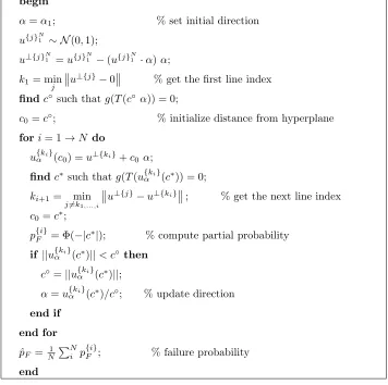
3.2. Adaptive Algorithm
An Adaptive algorithm, is developed in order to further improve the numer-180
ical efficiency for implementation in the generalized uncertainty environment.
The improvement concerns the efficiency in evaluating Equation 5. In contrast
to the standard algorithm, ALS uses a support sequence that is dynamically generated to adapt to the shape of the limit state surface. This makes the
algo-rithm significantly faster and capable of recognising the level of non-linearity of 185
the performance function. Moreover, ALS not only allows for variations in the
important direction but is also capable of identifying new important directions
to be updated during the simulation. Hence, only a very rough estimation of
the important direction is required at the start of the simulation.
The main features of ALS are: (i) it minimizes the number of samples along 190
the lines{j}to identifyc∗{j}, (ii) it adapts the important direction to the shape
of the limit state surface. The first feature is achieved developing an efficient line
search procedure and line selection. The second feature is achieved computing weights to each working direction.
As in standard implementations, ALS algorithm operates setting an (initial) 195
important direction α and generating a number NL of points u
{j}
α . First, a linej is deployed from the origin of the SNS approximately towards the failure
region as u{0}α (c) =c α. Then, the value c◦ ={c∈R|g(c◦α) = 0}, is used
for the starting point on the first line as u{1}α (c0) = u⊥{1} +c0 α. A line
search procedure, based on a Newton-Raphson iterative procedure, is applied 200
to identify the root c∗{j}, which is used to compute the partial probability
pF{j} = w(uα{j}) = Φ(−|c∗{j}|). Using the identified root, the procedure is
repeated as u{αj}(c0) = u⊥{j}+c∗{j−1} α, until all lines are processed. To
increase the efficiency, the algorithm does not process the lines randomly as
they are generated. Lines are selected according to a criterion based on the 205
Hence, in case of slightly non-linear limit state surface the distancesc∗{j} and
c∗{j−1}, for linesjandj−1 respectively, are expected to have approximately the
same value. To identify the neighbouring lines, the index of the line closest to the origin is computed ask1= arg min
j
u⊥{j}−0
. Subsequently, all the other
210
indices are calculated aski+1= arg min
j6=ki
u⊥{j}−u⊥{ki}
, and as illustrated in
the pseudo code of the algorithm in Figure 1.
3.3. Adaptation of the important direction
ALS allows to change the important direction without re-evaluating the
per-formance function along the processed lines. This feature is useful when there 215
is only little evidence of the optimal important direction, so that an
approx-imate direction can be set at the beginning of the simulation and a better
direction can be obtained during the simulation. An optimal direction generally
provides a more accurate estimate of the failure probability. The important
direction is usually associated with the design point ˜u∗ = minu∈{u|g=0} kuk,
220
i.e. the point on the limit state that carries the highest probability density.
As the ALS proceeds, the norm of the new state points ˜u = u⊥+c∗α can
be computed with nearly no cost, thus a new direction can be set as a more
probable point is identified on the limit state. Thus, if a point ˜u{αj} is found,
such that ||u˜{αj−1}|| > ||u˜{αj}||, then the new important direction can be set 225
as αnew = ˜u{αj}/||u˜
{j}
α ||. Changing the important direction does not affect the expected value of the failure probability. However, an improvement of the
important direction reduces the variance of the estimation.
3.4. Efficiency and accuracy
Adaptive Line Sampling shows an improvement in efficiency and accuracy 230
above the standard version. This is elucidated in a comparative study with a
reference solution obtained by Monte Carlo simulation. An explicit performance
function is used to test the methods, which is expressed asg(x) =−√xTx+a,
begin
α=α1; % set initial direction
u{j}N1 ∼ N(0,1);
u⊥{j}N1 =u{j}
N
1 −(u{j}
N
1 ·α)α;
k1= min
j
u⊥{j}−0
% get the first line index
findc◦ such thatg(T(c◦ α)) = 0;
c0=c◦; % initialize distance from hyperplane
fori= 1→N do u{ki}
α (c0) =u⊥{ki}+c0α;
findc∗ such thatg(T(u{ki}
α (c∗)) = 0; ki+1= min
j6=k1,...,i
u⊥{j}−u⊥{ki}
; % get the next line index
c0=c∗;
p{Fi}= Φ(−|c∗|); % compute partial probability
if ||u{ki}
α (c∗)||< c◦ then c◦=||u{ki}
α (c∗)||; α=u{ki}
α (c∗)/c◦; % update direction end if
end for ˆ
pF = N1 PNi p{ i}
[image:11.612.133.489.212.566.2]F ; % failure probability end
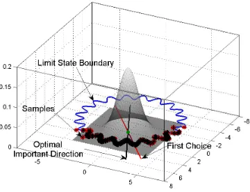
Figure 2: Directional change in standard normal space with ALS over the
non-linear limit state boundary defined in the original space by the performance
function:g(θ) =−(θ1+θ2)+d2(1+a sin(b tan−1(θ1, θ2))), whereθ1∼N(5,22),
θ2∼N(2,22),d= 10,a= 0.2 andb= 20.
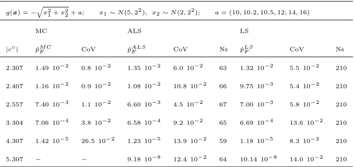
probability targets, by selecting different values ofain the performance function
g, as shown in Table 1. Note that, in this case, the values of probabilitypF =
Φ(−β) obtained by First Order Reliability Method [25] are biased because of the
concave shape of the limit state surface. An illustration of the performance of the
methods is shown in Figure 3a. A satisfactory level of accuracy (CoV = 5·10−2) 240
is achieved with just 65 samples using ALS compared to a necessary sample size
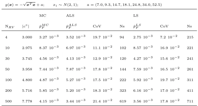
of 210 samples using LS. Secondly, the test is run fixing probability targets
(approximately to 10−3), while progressively increasing the number of random
variables, as shown in Table 2. The results of this second test, as illustrated in Figure 3b, show that Monte Carlo, is insensitive to the number of variables, 245
whilst the other methods show some sensitivity to the number of variables but
require significantly less samples to achieve the same level of accuracy. As
expected, in this second test, the probability of failure computed with the First
Order Reliability Method is inaccurate, as also shown in Table 2. In both cases,
g(x) =−qx2
1+x22+a; x1∼N(5,22), x2∼N(2,22); a= (10,10.2,10.5,12,14,16)
MC ALS LS
|c◦| pˆM CF CoV pˆALSF CoV Ns pˆLSF CoV Ns
2.307 1.49 10−2 0.8 10−2 1.35 10−2 6.0 10−2 63 1.32 10−2 5.5 10−2 210
2.407 1.16 10−2 0.9 10−2 1.08 10−2 10.8 10−2 66 9.75 10−3 5.4 10−2 210
2.557 7.40 10−3 1.1 10−2 6.60 10−3 4.5 10−2 67 7.00 10−3 5.8 10−2 210
3.304 7.06 10−4 3.8 10−2 6.58 10−4 9.2 10−2 65 6.69 10−4 13.6 10−2 210
4.307 1.42 10−5 26.5 10−2 1.23 10−5 13.9 10−2 59 1.18 10−5 8.3 10−2 210
[image:13.612.134.481.147.311.2]5.307 − − 9.18 10−8 12.4 10−2 64 10.14 10−8 14.0 10−2 210
Table 1: Test of ALS and LS on the bidimensional performance g(x) =
−px2
1+x22+a; comparison with the reference solution obtained via MC with
106samples.
10−7
10−6
10−5
10−4
10−3
10−2
100
102
104
106
108
1010
1012
p
F
number of samples
MC LS ALS
(a)
4 10 100 500
101
102
103
104
105
106
107
number of variables
number of samples
MC LS ALS
(b)
Figure 3: Number of samples required from ALS and LS compared to the
refer-ence solution obtained with MC and 106samples (a) for a decreasing probability
[image:13.612.144.464.443.590.2]g(x) =−√xTx+a; xi∼N(2,1); a= (7.0,9.3,14.7,18.1,24.8,34.0,52.5)
MC ALS LS
NRV |c◦| pˆM CF pˆALSF CoV Ns pˆLSF CoV Ns
4 3.000 3.27 10−3 3.52 10−3 19.7 10−2 94 2.75 10−3 7.2 10−2 215
10 2.975 8.37 10−3 6.97 10−3 11.1 10−2 102 8.57 10−3 16.9 10−2 221
30 3.745 4.56 10−3 4.13 10−3 12.9 10−2 120 4.27 10−3 15.6 10−2 241
50 3.958 7.44 10−3 7.87 10−3 17.8 10−2 144 7.59 10−3 16.5 10−2 261
100 4.800 4.87 10−3 5.27 10−3 17.5 10−2 222 5.92 10−3 19.7 10−2 311
200 5.716 5.85 10−3 5.20 10−3 18.3 10−2 323 6.16 10−3 17.0 10−2 411
[image:14.612.137.470.130.308.2]500 7.778 4.15 10−3 3.44 10−3 21.4 10−2 619 3.56 10−3 17.8 10−2 711
Table 2: Test of ALS and LS on the performance functiong(x) =−√xTx+a;
comparison with reference solution from MC with 106samples andCoV ≤0.03,
and increasing dimension of the limit state.
4. Sampling-based estimation of set-valued reliability
When imprecision is considered, the failure probability is obtained as interval
pF . In order to calculate the bounds of the failure probability, a global search in
the bounded setsQ1andQ2is performed. A naive approach to the problem for
searching in the above sets would be prohibitive in the majority of cases due to 255
the numerical effort incurred. In fact, two nested loops are required, where the inner loop estimates the failure probability and the outer loop searches for the
bounds of the probability. The ALS method not only makes the computation
of probabilities faster compared with Monte Carlo, but most importantly, can
be adopted to significantly ease the search procedure of failure probability. 260
4.1. The global search for lower and upper failure probabilities
The objective function for the global search in the setsQ1 and Q2 is given
search can be seen as an iterative procedure that converges after some steps,
towards the sought lower and upper failure probability bounds. 265
4.1.1. The search in the bounded set of distribution parametersQ1
The set Q1 of distribution parameters defines the set of all probability
dis-tribution functions to be considered in the analysis. Any element ofQ1 is
asso-ciated with a different value of failure probability. Nonetheless, the limit state
does not change as we search inQ1. This is because the limit state depends 270
upon the structural system and not upon the uncertainty model that defines
the probability distribution over the state variables. Since the important
direc-tion is defined as any direcdirec-tion pointing towards the failure domain, during the
search inQ1, an approximateαcan be set for the entire analysis, independently
from the distribution functions of the random variables. However, changing the 275
distribution functions modifies the location of the most probable point on the
limit state surface. Hence, the direction α, set at beginning of the analysis,
might not be the optimal one for all the distributions analysed. This motivates
the implementation of a flexible algorithm capable of searching and updating
new optimal directions. 280
Each step of the search procedure requires the estimation of a failure
proba-bility. In the standard approach a completely new simulation would be carried
out to find each of these failure probabilities. However, if the distribution
func-tions do not significantly change, it is not necessary to run a whole new
sim-ulation. For this reason, the proposed strategy includes a verification of those
changes during the search for the probability bounds. Taking advantage of the
bijective mappingTof the random variables between original and standard
nor-mal space, and of the fact that the limit state does not change as we search in
Q1, any point ˜u on the limit state can be transformed back onto the original
space, and then re-mapped to the SNS for the next simulation. When a new reliability analysis is started, the points on the limit state ˜u, previously found,
can be used to feed further analyses. Letαidenote the direction of the current
simulation, the failure probability
pF(i)= Z
Rn−1
w(u⊥αi)hN(u ⊥
αi)du
n−1 (6)
can be computed using the limit state points from the previous simulation
w(u⊥α
i−1) → w(u ⊥remap
αi ). However, the new values of w obtained with the
re-mapped points are no longer drawn from a probability distribution.
There-fore, in order to be able to compute the failure probability using the points from
previous simulations, a dummy probability density functionhX is constructed
285
around the re-mapped points on the hyperplane. The density functionhX is a
multi-modal distribution with density peaks centred on the re-mapped points
and are weighed using the metric properties of the SNS. The failure probability
can then be written as
pF(i+1)= Z
Rn−1
w(u⊥remapα i+1 )hN(u
⊥
αi)
hX(u⊥remapαi+1 )
hN(u⊥αi)
dun−1. (7)
By means of the ratio q= hX(u⊥remapαi )/hN(u ⊥
αi−1), the probability pF(i) can
290
now be computed using the information from simulationi−1 as
˜ pF(i)=
1 N
N
X
j
q{j} w(u⊥remapαi ) =
1 N
N
X
j
q{j} R(w(u⊥αi−1)), (8)
where,R(.) is a function that transforms variablew(u⊥αi−1) from the standard
space of simulationi−1 to the standard space of simulationi.
4.1.2. The search in the bounded set of structural parametersQ2
Imprecision of structural parameters, characterized by the bounded setQ2, 295
requires an extension of the procedure developed so far. In fact, the bounded
variablesx∈Rn2 change the shape of the limit state boundary, which needs to
be addressed with a second search as described in Equation (1). In this section,
we propose a strategy to include the variablesx∈ Q2 in the numerical
frame-work presented so far. The strategy consists of an extension to an augmented 300
probability space, where the interval variables are treated as dummy normal
In simple terms, this permits a combined consideration of the bounded setQ2
together with the bounded setQ1 in the same manner. Each dummy imprecise
random variable has an interval mean valueµx=x, and a real-valued standard 305
deviationσxto be fixed with some convenient value. By defining these dummy
imprecise random variables a thorough search can be performed in both setsQ1
andQ2simultaneously. The only requirement for the dummy imprecise random
variables is that the chosen value ofσx should neither be too large nor be too
small to avoid numerical issues in computing the failure probability. The stan-310
dard deviationσx can be set, for example, as a fraction of the interval radius
σx=k(x−x)/2, wherekcan be any value between 0 and 1. Once the argument
optima in the setsQ1 and Q2 are found, the associated bounds on the failure
probability are also known. Two more reliability analyses at the end of the
search, run on the argument optima, will be needed to find the failure probabil-315
ity bounds. Note that during this procedure sampling outside the intervals may
occur. However, points outside the intervals are solely used to drive the search
process. In cases where the physical model restricts the evaluation to the range
of the intervals, truncated normal random variables are used for the dummy
imprecise variables, which lower and upper limits are equal to the endpoints of 320
the intervals.
When the limit state surface is only slightly non-linear the search procedure
can be sensibly sped up. In fact, in this case the important directions in the
original space are all oriented towards the same region of the state space. This
implies that, as we search in Q1 and Q2, the coordinates of the important 325
directions may vary but do not change in sign. Therefore, the sign of the
coordinates of the important direction in the original space can be used to
identify the mean states that are the nearest and furthest from the limit state
surface. Let us denote these two states as conjugate states. Where the mean
state is the nearest to the limit state surface (upper conjugate state), it is also 330
where the failure probability attains its maximum. The contrary applies at the
furthest mean state from the limit state surface (lower conjugate state), where
distributions defined in terms of moments (first and second) and in terms of
parameters is necessary. If the probability distribution is defined in terms of 335
moments, the argument optima of the failure probability are obtained at the conjugate states, by selecting the maximum and minimum variance, respectively
for the minimum and maximum failure probability. This applies because we
can pick values at the corners at the hyper-cube defined in terms of moments,
without problems of dependency. If the probability distribution is defined in 340
terms of parameters, the search domain in the space of the moments may no
longer be a hyper-cube. In fact, in this case a conjugate state (either lower or
upper) corresponds to only one value of variance, which may not be at a corner
of the domain. However, lower and upper bounds of the failure probability
can still be found selecting the conjugate states and the maximum/minimum 345
variance independently, and find the associated parameter combinations.
5. Integration of the strategy in OpenCossan
The developed algorithm has been integrated into OpenCossan [26], which
is an open-source integrated numerical framework for uncertainty
quantifica-tion and risk analyses [24]. OpenCossan is coded exploiting the object-oriented 350
MatlabR environment, which makes it highly flexible using a modular
soft-ware architecture. Recalling that a class is an extensible case of objects and
properties [27], the strategy takes advantage of three main new classes, namely
AdvancedLineSampling,LineSamplingData andExtremeCase.
5.1. Class Advanced Line Sampling
355
The classAdvancedLineSamplingintegrates the methods for estimating
pre-cise failure probabilities. Provided a ProbabilisticModel, containing a
perfor-mance function, and an Input object, a reliability analysis can be performed
invoking the methodcomputeFailureProbability, as shown in Figure 4. In order
to optimize the performance and increase the robustness of
AdvancedLineSam-360
which implements a Newton-Raphson method to look for the roots of the limit
state surface,extractLineIndex, which searches the index of the nearest line to
the current one amongst the ones not already processed, and computePartial-Probabilities, which computes the probabilitiesp{Fi}= Φ(−|c∗{i}|) for every line
365
i= 1, ..., N. The design of these methods ensure the accuracy and robustness of
the algorithm. The methodcomputePartialProbabilities, for example, is
respon-sible for evaluating the expansionswand can be given the option of eliminating
individual lines during the search process. ThelineSearchmethod provides the
user with the choice to adjust the control parameters, such as the tolerance 370
on the values of g and the minimum step size, to control the accuracy of the
algorithm if necessary.
5.2. Class Line Sampling Data
The classLineSamplingData is a key-component in the economy of the
strat-egy. It stores the results obtained from every line in a structured and organized 375
way, it can be used to plot the results, and feed further analyses. This class is
essential also for the parallelization of the algorithm, in combination with the
methods merge and add, which allow to gather results coming from different analyses.
5.3. Class Extreme Case Analysis
380
Eventually, in order to search for lower and upper bounds of the failure
probability, the class ExtremeCase is created in OpenCossan. ExtremeCase
connects the inner solver running the ALS simulations with an optimizer such as
Genetic Algorithms. ExtremeCasemakes use of the methodoptimize to deploy
the optimization, and of the method ConstructSolutionSequence to formulate 385
the optimization problem. ConstructSolutionSequence is a central method for
the efficiency of the algorithm; it checks number and accuracy of simulations
Input
PerformanceFunction
ProbabilisticModel Model
+ apply ( )
+ computeFailureProbability ( )
AdvancedLineSampling
LineSamplingData
+ plotLines ( )
+ plotLimitState ( ) FailureProbability
Reliability
Simulations Inputs
Physical Model
[image:20.612.224.389.140.313.2]Outputs
Figure 4: Simplified UML diagram for the implementation of the Advanced Line
Sampling strategy in OpenCossan.
ImpreciseRandomVariable IntervalVariable
Input
PerformanceFunction
ProbabilisticModel Model
LineSamplingData
Optimum
SolutionSequence
+ runScript ( )
ExtremeCase
+ constructSolutionSequence ( )
+ optimize ( ) + mapping ( )
+ apply ( )
+ computeFailureProbability ( )
AdvancedLineSampling
Optimizer
FailureProbability LH, GA, BOBYQA
IntervalFailureProbability
Inputs
Physical Model
Reliability
Optimization
Output
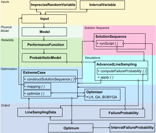
Solution Sequence
[image:20.612.178.434.395.613.2]Simulations
Figure 5: Simplified UML diagram with patterns for the implementation of the
6. Examples and applications
6.1. Synthetic example
390
To demonstrate the performance of the proposed method a synthetic exam-ple is presented. The approach developed in this paper, denoted as approach
A, is compared to a solution obtained through global optimization, denoted
as approach B. Both approaches are applied to calculate the interval failure
probability pF. In approach A the argument optima are detected using the 395
information of the important direction as explained in Section 4.1.2. The sign
of the important direction in the original space identifies the conjugate states
where the optima of the failure probability are located.
In approach B, the search procedure is driven by optimizers. The example is
solved using both Genetic Algorithm (GA) according to [28] and BOBYQA from 400
[29], as global and local searchers, respectively. With this approach a thorough
search in the setsQ1andQ2is performed. The objective function is given by the
failure probability, thus, at any iteration of GA/BOBYQA, a simulation with
ALS is performed. This approach can be run only because ALS requires just
few evaluations of the performance function to complete an iteration. Replacing 405
ALS with Monte Carlo would lead to hundreds of evaluations of the performance
function for each iteration, making approach B intractable.
Two cases are considered in this study, namely case (a) and case (b).
Case (a): The linear performance functiong(ξ, x) = 7 +ξ−2x,is evaluated.
It includes the imprecise random variableξ∈ C, where 410
C = {hN(ξ;µ, σ)| µ∈[0.9,1.3], σ∈[0.7,2.1]}, and the interval variable
x = [1, 3]. In this illustrative case the gradient ∇g = (1,−2), suggests the
initial important directionα = (1,−2)/√5. Approach A leads to the bounds
of the failure probability and the associated argument optima (x∗, x∗) = (x, x),
and p∗ = (µ, σ), p∗ = (µ, σ), as shown in Table 3. With approach B, using 415
GA with a population size of 50 individuals, an approximation of the of lower
and upper bound was obtained after 52 iterations, while BOBYQA delivered
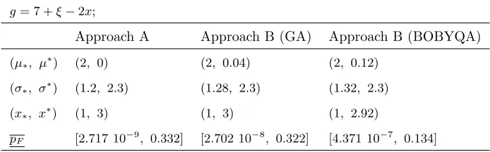
g= 7 +ξ−2x;
Approach A Approach B (GA) Approach B (BOBYQA)
(µ∗, µ∗) (2, 0) (2, 0.04) (2, 0.12)
(σ∗, σ∗) (1.2, 2.3) (1.28, 2.3) (1.32, 2.3)
(x∗, x∗) (1, 3) (1, 3) (1, 2.92)
[image:22.612.133.480.130.238.2]pF [2.717 10−9, 0.332] [2.702 10−8, 0.322] [4.371 10−7, 0.134]
Table 3: Results from Example I, case (a), argument optima and associated
failure probabilities for approaches A and B respectively.
g= 9 +ξTa1−xTa2;
a1= (1,4,2,0.1,0.2,0.6,5,0.01,0.2,0.3,0.25,0.14,0.8,3), a2= (−2,0.1,1)
Approach A Approach B (GA) Approach B (BOBYQA)
pF [1.795 10−9, 0.1452] [7.302 10−6, 0.0053] [2.538 10−5, 0.0046]
Table 4: Results from Example I, case (b), interval failure probability for
ap-proach A and B.
closed-form solution and it is clearly advantageous above approach B.
Case (b): The multidimensional linear performance function g(ξ,x) = 9 + 420
ξTa1−xTa2, where a1∈R14, anda2∈R3, is considered. The imprecise
ran-dom variablesξ∈R14are defined by the credal setC=hN(ξ;µ,σ)|µ∈µ,σ∈σ ,
whereµ= [0.1, 1]14, andσ= [1.2, 2.3]14, while the interval variablesx∈
R14
are defined by the bounded set x = [1, 3]3. Again, because of the linearity,
approach A delivers numerically exact results for the failure probability (equal 425
to the closed-form solution). As expected, approach B provides only a rough
approximation of the solution, as shown in Table 4. The global search becomes
inefficient when the dimensionality of the search domain grows, in the example
6.2. Large scale finite element model of a six-storey building
430
In this example the reliability analysis of a six-story building subject to wind
load is carried out. Three different models of uncertainty are considered with
increasing level of generality. Firstly, a standard reliability analysis, where the
inputs are modelled by precise probability distribution functions, is performed.
Secondly, the structural parameters are modelled as imprecise random variables 435
with the credal set C. In the third analysis both imprecise random variables
and intervals are considered for structural parameters.
An ABAQUS finite element model (FEM) is built for the six-story building,
as illustrated in Figure (6), which includes beam, shell and solid elements. The
load is considered as combination of a (simplified) lateral wind load and the self-440
weight, which are both modelled by deterministic static forces acting on nodes
of each floor. The magnitude of the wind load increases with the height of the
building. The FEM of the structure involves approximately 8200 elements and
66,300 DOFs. A total of 244 independent random variables are considered to
account for the uncertainty of the structural parameters. The material strength 445
(capacity) is represented by a normal distribution, while log-normal
distribu-tions are assigned to the Young’s modulus, the density and the Poisson ratio. In addition, the cross-sectional width and height of the columns are modelled
by independent uniform distributions. A summary of the distribution models is
reported in Table 5. 450
Component failure for the columns of the 6th storey is considered as failure
criterion. The performance function is defined as
f(θ) =|σI(θ)−σIII(θ)|/2−σy, (9)
i.e. as the difference between the maximum Tresca stress, whereσIII ≤σII ≤σI
are the principal stresses, andσy is the yield stress.
Standard reliability analysis. A reliability analysis is carried out with the precise 455
distribution models from Table 5, and using LS and ALS for comparison of
Figure 6: FE-model of the six-story building.
# U.V. Probability dist. Distribution Description Units
1 N(0.1, 0.001) Normal Column’s strength GPa
2−193 Unif(0.36,0.44) Uniform Sections size m
194−212 LN(35.0, 12.25) Log-normal Young’s modulus GPa
213−231 LN(2.5, 0.0625) Log-normal Material’s density kg/dm3
232−244 LN(0.25, 0.000625) Log-normal Poisson’s ratio
-Table 5: Precise distribution models for the input structural parameters.
the origin of the SNS. The identified important direction is displayed in figure 7,
where the first coordinate (the material’s strength) appears to be the most
important one. The other coordinates refer to the size of the cross-sections, the 460
Young’s modulus, the density, and the Poisson’s ratio, respectively (see Table
5). As illustrated in Figure (7), only a few uncertain variables (U.V.) dominate
the important direction; these are the Young’s modulus of columns of floor 6
(U.V. #199) and the density of the columns of floors 5 and 6 (U.V. #223 and
#224), along with the yield strength (U.V. #1). In this example, performing LS 465
with 30 lines (180 samples) leads to the failure probability of ˆpF = 1.30·10−4 and a coefficient of variation of CoV = 0.076. ALS leads to the probability
[image:24.612.136.489.304.418.2]1 50 100 150 200 244 −1
−0.8 −0.6 −0.4 −0.2 0 0.2 0.4
# R.V.
[image:25.612.185.427.134.266.2]coordinate value
Figure 7: Values of the 244 coordinates of the initial important direction in the
standard normal space.
with only 62 samples. Both methods estimate approximately the same value of
failure probability, but with quite a smaller number of model evaluations were 470
required by ALS.
Imprecision in distribution parameters (MI). The model of uncertainty is
ex-tended to include the credal set
C
hD(θ;p) |p∈R488, p∈ Q1 ,whereDare the probability distribution
models from Table 5, and 475
p= (µ1, σ1, ..., m244, v244) are the distribution parameters of these models
specified by the bounded setQ1=
×
488i pi. The interval parameters arerepre-sented asp=pc(1−),p=pc(1 +), using the interval centerpc= (p+p)/2 and the relative radius of imprecision. These intervals [p, p] are summarized
in the bounded setQ1. In the example, all interval parameters, are modeled
480
with the same relative imprecision. In order to explore the effects of on the
results, we use a fuzzy set to consider a nested set of intervals ˜p =
[p, p]
for the parameters in one analysis. The amplitude (width) of the intervals is
controlled by to obtain fuzzy sets ˜p as shown in Figure 9. An upper limit
for the relative uncertainty is set as = 0.075. Specifically, the intervals for 485
3 3.2 3.4 3.6 3.8 4 4.2 4.4 4.6 4.8 −1.5
−1 −0.5 0 0.5 1
x 107
distance from hyperplane
performance values
(a)
4 6 8 10 12 14 16 18 −1.5
−1 −0.5 0 0.5 1 1.5
2x 10
7
Norm (L−2) of state points in SNS
performance values
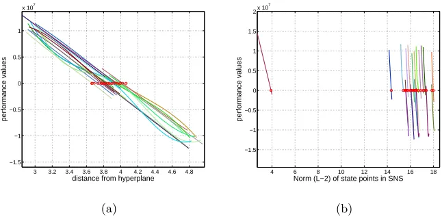
[image:26.612.140.463.127.287.2](b)
Figure 8: Values of the performance function along the lines in SNS for one
reliability analysis of the multi-storey building. In Figure (a), the lines are
plotted aginst the distance from the hyperplanec, while in Figure (b) the lines
are plotted against the L-2 norm||u˜||of the state points ˜u=T(˜θ).
with the generalized model of uncertainty is performed using the important
direction determined in the original space.
From a rough search in the setQ1, it was found that the important direction did not significantly change in the original space. This allowed us to identify the 490
argument optima in the bounded setQ1as combination of extreme moments as
described in Section 4.1.2. These upper and lower conjugate states are also
asso-ciated with the maximum and minimum of the failure probability, respectively.
The result of the robust reliability analysis is shown in Figure 9b and in Table
6. From Table 6 can be appreciated that the number of samples required by 495
one robust reliability analysis, on average, is approximately 254, which is even
less than number of samples required by two standard reliability analyses using
Line Sampling (∼360 samples). This is an astounding results considering that
a standard approach, driven by two nested loops, would have required several hundreds of thousands of samples. The failure probability is obtained as a fuzzy 500
set, which includes the standard reliability analysis as special case with= 0.
Lower Bound Upper Bound
p
F CoV pF CoV Ns
0.000 1.42 10−4 9.2 10−2 1.42 10−4 9.2 10−2 126
0.005 5.75 10−5 8.7 10−2 2.63 10−4 7.1 10−2 257 0.010 4.57 10−5 33.6 10−2 5.30 10−4 11.5 10−2 250
0.025 1.75 10−6 8.8 10−2 3.22 10−3 5.3 10−2 253
0.050 2.27 10−8 57.0 10−2 3.88 10−2 5.4 10−2 255
[image:27.612.165.448.125.273.2]0.075 1.88 10−11 12.2 10−2 2.02 10−1 3.5 10−2 254
Table 6: Results of the robust reliability analysis of the multi-storey building from model MI, obtained in terms of lower and upper bounds of the failure
probability.
input for the same membership level, and each membership level is associated
with a different value, see Figure 9b. In a design context, this result can be
used to identify a tolerated level of imprecision for the inputs given a constrain 505
on the failure probability. For example, fixing an allowable failure probability
of 10−3, the maximum level of imprecision for the distribution parameters is
limited to 1%, see Figure 9.
Imprecision in both distribution parameters and structural parameters (MII).
In this example the section sizesx∈R192 are considered as interval variables,
510
while the remaining structural parametersζ∈R52are considered as imprecise
random variables. The model of uncertainty comprises the setC
hD(ζ;p) |p∈R104, p∈ Q1 ,
and the setQ2=
×
192i xi. The imprecise distribution parameters are modeledusing the radius of imprecision, as in model caseMI, see Table 8. An upper
limit for the relative radius of imprecision is set to = 0.03. In the analy-515
sis, a rough search in the setsQ1 and Q2 allowed us again to identify a main
important direction for determining the argument optima associated with the
minimum and maximum value of failure probability. The result is shown in
0 0.1 0.2 0.3 0.4 0.5 0.6 0.7 0.8 0.9 1 membership
pc(1- )3 pc pc(1+ )3 3=0.075 3=0.05 3=0.025 3=0.01 3=0.005 3=0 (a)
100−12 10−10 10−8 10−6 10−4 10−2 100
0.1 0.2 0.3 0.4 0.5 0.6 0.7 0.8 0.9 1 membership pF (b)
Figure 9: (a) Fuzzy paramters ˜p={pc [1−j, 1 +j]}
6
j=1and (b) fuzzy failure
probability obtained with model MI as set of results for different levels of imprecision.
samples required by one robust reliability analysis, on average, is approximately 520
254. Again, it is necessary to point out that a standard approach, driven by two
nested loops, would have required several hundreds of thousands of samples to
compute the interval failure probability.
To explore the sensitivity against imprecision of the uncertain parameters,
the failure probability is obtained as a fuzzy set. The relative radii of imprecision 525
={0,0.01,0.015,0.020,0.025,0.03} are considered to construct a fuzzy model
for all parameters, see Figure 10a. The intervals for the structural parameters
xinQ2, describing the size of the cross-sections, are independent of, see Table 8. Once more, the analysis may serve as a design tool to find the tolerable level
of imprecision provided a threshold of allowable probability. 530
Here, the uncertainty due to imprecision is larger, because the whole range of
the intervals is taken into account for the cross-sections. As in the previous case,
a rough search in the setsQ1 andQ2 allowed us to identify a main important
direction for selecting the argument optima producing minimum and maximum
value of failure probability. Values of failure probability, obtained with = 535
[image:28.612.136.479.134.274.2]#U.V. Prob. dist. p=pc[1−, 1 +] Description Units
1 N(µ, σ) µc= 0.1 σc= 0.01 Columns’ strength GPa
2−193 Unif(a, b) ac= 0.36 bc= 0.44 Sections’ size m
194−212 LN(m, v) mc= 35 vc= 12.25 Young’s modulus GPa
213−231 LN(m, v) mc= 2.5 vc= 0.0625 Material’s density kg/dm3
232−244 LN(m, v) mc= 0.25 vc= 0.000625 Poisson’s ratio
-Table 7: Inputs definition from uncertainty model MI; the relative radius of
imprecision for this model is set as={0,0.005,0.0.01,0.025,0.05,0.075}.
#U.V. Uncertainties type p=pc [1−, 1 +], x= [x, x]
1 distribution N(µ, σ2) µc= 0.1 σ2c= 0.001 2−193 interval x x= 0.36 x= 0.44
194−212 distribution LN(m, v) mc= 35 vc= 12.25
213−231 distribution LN(m, v) mc= 2.5 vc= 0.0625
[image:29.612.133.488.128.240.2]232−244 distribution LN(m, v) mc= 0.25 vc= 0.000625
Table 8: Inputs definition from uncertainty modelMII; the relative radius of imprecision for this model is set as={0,0.01,0.015,0.020,0.025,0.03}.
7. Conclusions
In this paper an efficient computational strategy for computing set-valued
failure probabilities was presented. The approach couples advanced sampling-based methods with optimization procedures. An Adaptive algorithm was devel-540
oped and implemented into the broader Advanced Line Sampling method. The
global search for lower and upper bounds of the failure probability was driven
using the information provided by an averaged important direction, obtained in
the original space of the state variables, to identify the conjugate states. It was
[image:29.612.148.459.312.423.2]Lower Bound Upper Bound
p
F CoV pF CoV Ns
0.000 4.70 10−7 10.2 10−2 6.73 10−3 11.5 10−2 259
0.010 2.28 10−7 13.4 10−2 9.71 10−3 12.2 10−2 247
0.015 1.10 10−7 10.3 10−2 1.11 10−2 7.6 10−2 255
0.020 5.19 10−8 13.1 10−2 2.08 10−2 14.6 10−2 255
0.025 2.51 10−8 9.97 10−2 2.72 10−2 15.3 10−2 249
[image:30.612.173.436.152.298.2]0.030 1.40 10−8 9.94 10−2 3.21 10−2 6.5 10−2 254
Table 9: Results of the robust reliability analysis of the multi-storey building
from model MII, obtained in terms of lower and upper bounds of the failure
probability.
0 0.1 0.2 0.3 0.4 0.5 0.6 0.7 0.8 0.9 1
membership
pc(1- )3 pc pc(1+ )3
3=0.03
3=0.075
3=0.05
3=0.025
3=0.01
3=0
(a)
100−8 10−7 10−6 10−5 10−4 10−3 10−2 10−1 0.1
0.2 0.3 0.4 0.5 0.6 0.7 0.8 0.9 1
membership
pF
(b)
Figure 10: (a) Fuzzy distribution parameters ˜p={pc [1−j, 1 +j]}
6
j=1 and
(b) fuzzy failure probability from model MII obtained as set of results for
[image:30.612.136.478.436.579.2]reduces the computational time of robust reliability analysis without
compro-mising the accuracy of results. The efficiency of the proposed method allows
its application on real scale engineering problems, while its accuracy guarantees the computation of informative intervals of failure probability.
[1] O. Ditlevsen, H. O. Madsen, Structural reliability methods, Vol. 178, Cite-550
seer, 2007.
[2] P. Bjerager, On computation methods for structural reliability analysis,
Structural Safety 9 (2) (1990) 79–96.
[3] J. Hurtado, A. Barbat, Monte carlo techniques in computational stochastic mechanics, Archives of Computational Methods in Engineering 5 (1) (1998) 555
3–29.
[4] N. Metropolis, S. Ulam, The monte carlo method, Journal of the American
statistical association 44 (247) (1949) 335–341.
[5] R. Melchers, Importance sampling in structural systems, Structural safety
6 (1) (1989) 3–10. 560
[6] S. Engelund, R. Rackwitz, A benchmark study on importance sampling
techniques in structural reliability, Structural Safety 12 (4) (1993) 255–
276.
[7] O. Ditlevsen, P. Bjerager, R. Olesen, A. Hasofer, Directional simulation in
gaussian processes, Probabilistic Engineering Mechanics 3 (4) (1988) 207– 565
217.
[8] O. Ditlevsen, R. E. Melchers, H. Gluver, General multi-dimensional proba-bility integration by directional simulation, Computers & Structures 36 (2)
(1990) 355–368.
[9] P. Koutsourelakis, H. Pradlwarter, G. Schu¨eller, Reliability of structures 570
in high dimensions, part i: algorithms and applications, Probabilistic
[10] P. Koutsourelakis, Reliability of structures in high dimensions. part ii.
the-oretical validation, Probabilistic engineering mechanics 19 (4) (2004) 419–
423. 575
[11] S.-K. Au, J. L. Beck, Estimation of small failure probabilities in high
di-mensions by subset simulation, Probabilistic Engineering Mechanics 16 (4)
(2001) 263–277.
[12] A. Der Kiureghian, Analysis of structural reliability under parameter
un-certainties, Probabilistic engineering mechanics 23 (4) (2008) 351–358. 580
[13] A. Der Kiureghian, P.-L. Liu, Structural reliability under incomplete
proba-bility information, Journal of Engineering Mechanics 112 (1) (1986) 85–104.
[14] M. Beer, S. Ferson, V. Kreinovich, Imprecise probabilities in engineering analyses, Mechanical Systems and Signal Processing 37 (1) (2013) 4–29.
[15] R. Moore, W. Lodwick, Interval analysis and fuzzy set theory, Fuzzy Sets 585
and Systems 135 (1) (2003) 5–9.
[16] S. Ferson, V. Kreinovich, J. Hajagos, W. Oberkampf, L. Ginzburg,
Ex-perimental uncertainty estimation and statistics for data having interval
uncertainty, Sandia National Laboratories, 2007.
[17] D. Moens, D. Vandepitte, A survey of non-probabilistic uncertainty treat-590
ment in finite element analysis, Computer methods in applied mechanics
and engineering 194 (12) (2005) 1527–1555.
[18] Y. Ben-Haim, A non-probabilistic concept of reliability, Structural Safety
14 (4) (1994) 227–245.
[19] B. M¨oller, W. Graf, M. Beer, Fuzzy structural analysis using α-level opti-595
mization, Computational Mechanics 26 (6) (2000) 547–565.
[21] M. Zaffalon, The naive credal classifier, Journal of statistical planning and
inference 105 (1) (2002) 5–21.
[22] C. Jiang, X. Han, G. Lu, J. Liu, Z. Zhang, Y. Bai, Correlation analysis 600
of non-probabilistic convex model and corresponding structural
reliabil-ity technique, Computer Methods in Applied Mechanics and Engineering
200 (33) (2011) 2528–2546.
[23] M. Valdebenito, H. Pradlwarter, G. Schu¨eller, The role of the design point
for calculating failure probabilities in view of dimensionality and structural 605
nonlinearities, Structural Safety 32 (2) (2010) 101–111.
[24] E. Patelli, H.M.Panayirci, M. Broggi, B. Goller, P. Beaurepaire, H. J.
Pradl-warter, G. I. Schu¨eller, General purpose software for efficient uncertainty
management of large finite element models, Finite Elements in Analysis and Design 51 (2012) 31–48.
610
[25] K. Breitung, Asymptotic approximations for multinormal integrals, Journal
of Engineering Mechanics 110 (3) (1984) 357–366.
[26] E. Patelli, M. Broggi, M. de Angelis, M. Beer, OpenCossan: An efficient
open tool for dealing with epistemic and aleatory uncertainties, ACSE,
Proccedings of ICVRAM-ISUMA, Liverpool 14-16 July 2014. In press. 615
[27] C. Larman, Applying UML and Patterns: An Introduction to
Object-Oriented Analysis and Design and Iterative Development, 3/e, Pearson Education India, 2012.
[28] D. E. Goldberg, et al., Genetic algorithms in search, optimization, and
machine learning, Vol. 412, Addison-wesley Reading Menlo Park, 1989. 620
[29] M. J. Powell, The bobyqa algorithm for bound constrained optimization
without derivatives, Cambridge NA Report NA2009/06 (2009), University