Bayesian
Language
Games
Bas Cornelissen
Bayesian Language Games
Unifying and evaluating agent-based models
of horizontal and vertical language evolution
MSc Thesis
(Afstudeerscriptie)
written by
Bas Cornelissen
(born 26 February 1992 in Utrecht)
under the supervision ofWillem Zuidema, and submitted to the Board of Examiners
in partial fulfillment of the requirements for the degree of
MSc in Logic
at theUniversiteit van Amsterdam.
Date of the public defense: Members of the Thesis Committee:
Abstract.
Human language is one of the most intricately structured
communication system in the natural world. Over the last decades
re-searchers in various fields have developed the idea that languages are
primarily shaped by processes of cultural evolution, and that these
pro-cesses can account for the structure of language. Computational
mod-els play an important role in their arguments. This thesis asks what those
models can teach us about cultural language evolution. To that end, the
first part of this thesis connects the two main branches of agent-based
models, naming games and iterated learning, in a new
Bayesian language
game
. The game gives a unified view on the field and suggests a
charac-terisation of the behaviour exhibited by the main agent-based models of
language evolution. It moreover addresses shortcomings of earlier
mod-els. We find lineage-specific languages reflecting the innate biases of the
learners. The second part of this thesis aims to compare that behaviour
with the evolution of actual language. Numeral systems are argued to
be an ideal empirical test case for models of cultural language evolution.
We revisit Hurford’s pioneering work on the modelling of the emergence
of numeral systems, and discuss some further results.
. Iterated Learning
2.1. Early iterated learning models . . . 16
2.2. Iterated learning with Bayesian agents . . . 18
2.3. Convergence to the prior . . . 21
2.4. Convergent controversy . . . 24
2.5. Conclusions . . . 27
. Naming Games 3.1. The basic naming game . . . 30
3.2. The minimal strategy . . . 31
3.3. Lateral inhibition strategies . . . 34
3.4. Proof of convergence . . . 35
3.5. Conclusions . . . 38
. Bayesian Language Games 4.1. The Bayesian naming game . . . 42
4.2. The Dirichlet-categorical naming game . . . 44
4.3. Phenomenology of the dc naming game . . . 46
4.4. Language and production strategies . . . 49
4.5. Bayesian language games . . . 51
4.6. Characterising Bayesian language games . . . 53
4.7. Conclusions . . . 56
. Numeral systems 5.1. Balancing expressivity and simplicity . . . 60
5.2. An introduction to numeral systems . . . 62
5.3. The evolution of numeral systems . . . 67
5.4. Conclusions . . . 69
. Emergent numeral systems 6.1. Hurford’s base games . . . 72
6.2. Domain adaptivity in the base games . . . 75
6.3. Counting games . . . 79
6.4. Conclusions . . . 82
. Conclusions 7.1. Main contributions . . . 89
7.2. Future work . . . 90
Appendices A. Converging Markov Chains . . . 94
B. Lateral Inhibition Strategies . . . 97
C. Mathematical details of Dirichlet-categorical ng . . . 98
C.1. Dirichlet and categorical distributions . . . 99
C.3. Measuring the distance between languages . . . 102
C.4. Bayesian updating and lateral inhibition . . . 103
D. Parameter space of the dc language game . . . 104
E. A discrete Weibull model of population turnover . . . 105
F. Reformulating the packing strategy . . . 109
G. Base games . . . 113
G.1. Implicit biases in the additive naming game . . . 113
G.2. Properties of the additive base game . . . 115
The cultural
origins of
Communication abounds in the natural world, but few, if any, communication sys-tems are so intricately structured as human language. We can understand the meaning of a sentence that has never been uttered before, because we understand the words it consists of and the way in which they are combined — that is to say that language is
by and largecompositional. The words, morphemes, themselves also have an internal
structure: they consist of phonemes, combined in a accordance with a combinatorial, phonological system specific to the language. The semantic and phonological combi-natorics together give language what Hockett (1960) dubbed a ‘duality of patterning’ — a design feature not commonly found in communication systems of other species.
Most animal communication systems areholistic: every vocalisation has one specific
function, and no further internal structure (Zuidema 2013). There are, it seems, few interdependencies between vocalisations. But language is quite different: just about any two sentences will have many interdependencies in their phonology, morphology, hierarchical structure, and so on. It is in this sense that language has a distinct system-aticity(Kirby 2017).
Now, the Big Question is this: where does it come from? And, indeed, why only us? Well, we find ourselves in good company. Robert Berwick and Noam Chomsky (2017) have been thinking about the same question, and leave us no doubt how we should
not try to account for the structure of language: “by means of a cultural-biological
interaction”. No, “this latter effort fails in all respects”. Some of that work is “trivially inadequate”, or otherwise the “Kirby-type models”, “the Kirby work” and “the Kirby line of research” do of course “not say anything about the initial origin of compositionality”. Good, good! More than enough reason to write a thesis about this “Kirby type work” — and in passing perhaps even cite more than two of his papers. But let’s leave the polemics there. After all, what greater good do they really serve?
Berwick and Chomsky (2017) raise some fair concerns, for example regarding the testability and empirical validity of the Kirby-type theories. Or regarding their ex-planatory power: if your ‘agents’ already know, say, context-free grammars, and they ‘evolve’ a compositional language, does your model explain anything? Are you then, if anything, addressing the evolution of universal grammar, or just modelling language change? These are all valid concerns — or so I think, since I address some of them in this thesis, too. But reading Berwick and Chomsky’s paper — I haven’t read the book yet — one starts to understand what it means if two scientific traditions have lost their common ground and have started talking about radically different things, only superficially using the same words.
Kirby-type work turned that around: how do languages have to change, in order to fit in our brains (Christiansen and Chater 2016a)? Rather than evolving brains, let’s think about evolving languages.
For this to even make sense, one has to drastically change the, let’s say, Chomskyan conception of language. Language now becomes a complex adaptive system in its own right, that is subject to all kinds of pressures, at multiple different levels and timescales simultaneously (Kirby and Hurford 2002; Christiansen and Chater 2016a; Smith 2014; Kirby 2017; Steels 2016). On a biological level and evolutionary timescale the innate mechanisms that underly human cognition and language need to develop. At an in-dividual level and much shorter timescale, humans acquire language, constrained by what their biological makeup can accommodate. These learning biases influence, on a cultural level and historic timescale, the cultural dynamics of language. Universals that emerge through processes of cultural evolution in turn shape the fitness landscape and indeed, interactions exist within in and across all levels. Rather than looking solely at the biology of language, the question is how biology can interact with acquisition and use. The idea developed is that “language has been adapted through cultural trans-mission over generations of language users to fit the cognitive biases in inherent in the mechanisms used for processing and acquisition” (Christiansen and Chater 2016b, p. 12).
Returning to Berwick and Chomsky (2017), I think they are quite right to point out that this work “does not really tackle questions about the evolution of UG, but rather questions about how particular languages change over time, once the faculty of lan-guage itself is in place”. I doubt Kirby would disagree. Indeed, this is the entire point. Since if it turns out that languages tend to change over time in a somewhat
system-atic way thatexplainstheir structure, then the explanatory burden is lifted from the
faculty of language. And this is precisely what the Kirby-type theories argue for: that biology does not have to carry the entire explanatory load, but that a fair share of
lin-guistic structure can be explained by a process ofcultural evolution. As Kirby (2017)
concludes, “we expect the language faculty to contain strong constraints only if they are domain general (e.g. arising from general principles of simplicity) and that any domain-specific constraints will be weak.” If anything, the Kirby-type work is in the business of explaining away UG, rather than explaining it.
Now, the evolution of language is a notoriously hard problem — I belief this is where
one is supposed to mention theSociété— but how does one go about if language is
moreover a complex adaptive system? Using mathematical and computational mod-els is one solution. Modelling makes all assumptions absolutely transparent, allows one to verify their coherence and consistency and generate new hypotheses, or even predictions (Jaeger et al. 2009). Accordingly, models have figured prominently in the literature on cultural language evolution. And that is where the habitat of this thesis is
to be found. What can these models of language evolution actually learn us about
lan-guage evolution? That is the heart of this thesis, but as such, the question is too open ended. I therefore break up the question in two parts.
behaviour. The ‘substantial share’ is easily identified, since the field falls apart
in two (strictly separated) traditions. Chapter 2introduces the ‘vertical’
tradi-tion arounditerated learning. This is the Kirby-type work that addresses how
vertical transmission between generations can shape language. Chapter 3
in-troduces the ‘horizontal’ tradition aroundnaming games, which focusses on the
self-organising power resulting from local interactions within a generation.
Al-though the traditions are strictly separated, I will argue inchapter 4that their
models are very similar. To do so, I take inspiration from Bayesian models of
iterated learning and propose theBayesian language game. By further changing
the population model I can interpolate between both traditions and thus analyse their behaviour in a single unified framework. I moreover argue that it addresses some of the problems left open by Bayesian models of iterated learning. 2. How does that behaviour relate to actual evolved language?Once it is clear what
kind of behaviour these agent-based models exhibit, one should ask what this learns us about language evolution. But how can one start answering such a
question without an empirical test case? Inchapter 5I therefore argue that
nu-meral systems are a good test case, and explain in some detail what the structures
are one should try to explain. Inchapter 6I make a first start with simulating
the emergence of numeral systems, which largely amounts to revisiting and ex-tending the pioneering work of James Hurford.
The reader might want to note that the summaries at the start of every chapter further flesh out this outline.
The problem of language evolution challenges many disciplinary boundaries. This thesis alone borders at least several branches of linguistics, statistical physics, biology, probability theory and Bayesian (cognitive) modelling. When starting with the cur-rent work, I was new to pretty much all of these fields (except perhaps some courses in the latter two fields) and many important results might very well have escaped my attention. But some things I deliberately left out, or only touch on in passing. These include (1) models of biological evolution, (2) evolutionary game theory, (3) genetic algorithms, (4) evolution of ug, (5) empirical studies of transmission chains and (6) experimental semiotics. Neither will I further discuss broader debates, of which the Berwick and Chomsky paper is part. Instead, I try to address issues in the field of agent-based modelling of language evolution on its own terms. Indeed, the reader will notice that focus in the majority of this thesis is decidedly on the models, more so than on possible interpretations thereof. This partly reflects personal interest, but more impor-tantly, I belief interpretations of models should, insofar as possible, built on a sound understanding of the model themselves. That is what I hope this thesis, if anything, contributes to.
I have made the source code of all experiments publicly avail-able via bascornelissen.nl/msc-thesis (including all figures and LaTeX files). A refer-ence to the ‘raw’ data from all experiments can also be found there. The captions of
many figures contain a code likebng06orfig03. This identifies the experiment or
Throughout the thesis I use several notational conventions. Vectors are
written in boldface, as in x = (x1, . . . ,xK), and indexed bykif they have length
K. Sometimes it will be convenient to abbreviatex0 :=
∑K
k=1xk. We often need
to decorate variables with time-indications. The most consistent unambiguous solu-tion,x(t),x(t)
k etc., often clutters the notation. Therefore, vectors (boldface) simply get
their indication in the subscript (x1,x2, . . . ,xt, . . .) and I only use the superscript(t)
when confusion can arise, as inx(kt). IfXis a random variable with distribution Dist parametrized byλ, then byX∼Dist(λ)we mean thatpX(x) =Dist(x| λ)where the latter is the density (mass) function. We mostly drop the random variables and write
p(x)andp(x| z)rather thanpX(x)andpX|Z(x| z). Normalizing constants are often irrelevant and we writep(x)∝f(x)to indicate proportionality, i.e. thatp(x) =1/C·f(x)
whereCdoes not depend onx. With regard to sets,N,Z,Rdenote the natural numbers,
integers and reals. IfAandBare sets, their Cartesian product isA×BandBAdenotes
the set of all functionsf : A → B. ‘Spaces’ typically have a calligraphic character, so
xlies inX and parameters tend to be Greek. Finally,xis nearly always an observable
variable (e.g. an utterance),zand unobservable variables (e.g. internal representation
of a language),ma meaning andsa signal.
Iterated
Learning
Could it be that structure in language emerges because it is transmitted
from one generation to the next? Is cultural
transmission
the force
shap-ing language? Early models of iterated learnshap-ing suggested precisely that.
Bayesian models improved the early work by separating the biases of the
learners from the effects of transmission. But they also indicated that
cultural evolution only allows the prior biases to surface, a result that
sparked a small controversy. The ‘convergence to the prior’ was shown to
break down in more complicated populations, again creating room for the
shaping force of cultural evolution. This chapter introduces the iterated
learning tradition and ends with a list of desiderata for models of cultural
language evolution. The list serves as a guide to the remainder of this
thesis.
. . Early iterated learning models . . . 16
. . Iterated learning with Bayesian agents . . . 18
. . Convergence to the prior . . . 21
. . Convergent controversy . . . 24
F . In the iterated learning model, the language produced by the previous generation serves as the primary linguistic data for the next.
Adapted from Kirby ( ).
θ1
x1
θ2
x2
θ3
x3
Language (internal)
Utterances (external)
Generation Generation Generation
Early iterated learning models
In the early years of this century, James Hurford, Simon Kirby, Kenny Smith and
oth-ers, developed the idea that cultural transmission, in the form ofiterated learning(il),
could be the source of structure in language. Early work in this tradition tried to isolate a “minimal set of assumptions and hypotheses with which linguistic structure can be explained” (Brighton 2002). The result was a simple model of cultural transmission between generations consisting of a single agent each. In the model, language alter-nates between an internal representation (i-language in Chomskyan parlance; Chom-sky 1986, pp. 19–24) or an external representation in the form of actual utterances (e-language), as figure 2.1 illustrates. The first agent (the parent) is presented with sev-eral objects for which it produces some utterances. Those utterances form the primary
linguistic data from which the second agent (the child) has to learn a language.1
The utterances alone are not enough, unless you assume the child can mind-read. Instead meaning-signal pairs are often communicated.
The child goes on to become the parent of the next generation, forms expressions for several (other) objects, which are observed by the next agent, and so on.
Every generation learns a language by observing the language of the previous genera-tion, who themselves learned it from the generation before them. The target of learning is therefore the outcome of the same learning process and this gives rise an evolution-ary dynamics on the cultural level: the fact that a language has to be learned over again shapes the language itself to become better learnable, hence better transmissible. And key to better transmission, many studies suggested, was the acquisition of some form of systematicity. Paraphrasing Hurford (2000), language appeared to be structured, because cultural transmission favours systematicity.
, This conclusion was primarily based on
com-puter simulations of the emergence of compositionality which I briefly want to discuss. Suppose, following Brighton (2002), that agents are positioned in an environment with
various objects. The objects haveFpossible features, each takingVvalues, and thus
correspond to points in aF-dimensional meaning spaceM. The features might be
color and shape, taking values triangular, rectangular or circular and orange, blue and
black respectively. A language associates meaningsm ∈ Mto signalssin a spaceS
of signals, typically strings over some alphabet. Certain languages are compositional, meaning that the signals can be decomposed in subsignals that each bear one aspect
of the meaning. Compositional languages should be distinguished fromholistic
2.1. Early iterated learning models
Consider the following language with alphabet{t,r,c, o,b,k}:
(△, )7→to, (△, )7→tb (△, )7→tk
(□, )7→so, (□, )7→sb (□, )7→sk
(#, )7→co, (#, )7→cb (#, )7→ck
This language is clearly compositional, since the first subsignal indicates the shape, (triangle,rectangle,circle) and the second subsignal the color (orange,blue, black). In fact, that description is much more efficient:
△ 7→t, □7→s, #7→c
7→o, 7→b 7→k
Rather than listing the signals corresponding to each of theVF = 33meanings (the
worst case scenario for a holistic language), a compositional languages can be
com-pressedtoF·V=2·3 rules listing to whichsubsignal every feature maps. That also
means that one can faithfully reconstruct a compositional language fromF·Vsignals,
whereas it would need to observeallsignals to reconstruct a holistic language (in the
worst case). A compositional language is, in short, morecompressibleand as a result
bettertransmissible.
In reality, children do not observe their entire language (e.g. all English sentences), but only a subset of it. They face a
transmission bottleneck2
In fact, various different bot-tlenecks have been put forward; see Cornish ( , ch. ) for an overview and a discussion of the empirical findings regarding the presence of such a bottleneck. better known as thepoverty of the stimulus. If there is no such
bottleneck all languages can be transmitted in their entirety, and faithfully so. The lan-guage can consequently not be changed by transmission and the initial lanlan-guage marks asteady state, maintained throughout all future generations. In the presence of a bot-tleneck, however, the learner is forced togeneralizethe observed data to a full language, in which case systematic errors can slowly accumulate.
The exact generalisation mechanism can take many different forms, such as (heuris-tic) grammar induction (Kirby 2001; Zuidema 2003), training a neural network (Kirby and Hurford 2002; Smith 2002) or constructing a finite state transducer (Brighton 2002). All these mechanisms try to discern some structure (e.g. compositionality) in the language. Sometimes, that allows the child to produce signals for unobserved meanings. But in other cases, the child is forced to invent a new signal. Inciden-tally, the new signal introduces a structure previously absent in the language. The next generation is then more likely to infer a language that reproduces that structure. As time passes, the differences between successive generations shrink and the language becomes more and more stable: the transmission bottleneck forced the language to be-come better transmissible. This is how the poverty of the stimulus solves the poverty of the stimulus (cf. Zuidema 2003).
a medium-sized training set leading to structured meaning-signal mappings. The fact that these, and many other, different models gave rise to similar behaviour is in itself striking. But it also makes it difficult to decipher what exactly is going on.
The shape-color example gives a hint, since there is a language much more
compress-ible than a compositional one: the degenerate language that expresseseverymeaning
with the same signal. The fact that none of the early studies seem to have produced degenerate languages, suggests that a bias against those must have been present (Cor-nish 2011). Or, conversely, that the learning algorithms implicitly pressured towards compositional languages. This opens up the possibility that “cultural evolution does no more than transparently map properties of the biology of an individual to properties of language” (Kirby 2017). Kirby points out that there are reasons to doubt this conclu-sion: The size of the bottleneck and the structure of the domain for example influence the simulations. Nonetheless, it became clear that in order to make claims about the
shaping force of cultural evolution, one needs to know 1) what theimplicit biasesin
the model are, 2) what the biases of the agents are and 3) how those interact with the cultural process.
Iterated learning with Bayesian agents
In 2005, Thomas Griffiths and Michael Kalish reinterpreted the iterated learning model in a population of Bayesian agents. One reason for doing so is that it connects the it-erated learning model to a rich Bayesian modelling tradition in cognitive science (see e.g. Perfors et al. 2011; Goodman and Tenenbaum 2016; Griffiths, Kemp, and Tenen-baum 2008) and the formal models of human behaviour that have been proposed there. The Bayesian model of Griffiths and Kalish also solved the issues arising from implicit
biases, since itexplicitlyencodes the biases of the learners. Moreover, the authors
man-aged to characterise the long-term behaviour of the model —convergence to the prior—
which sparked a small controversy. In the years that followed, the Bayesian paradigm appears to have surfaced as the primary approach to modelling iterated learning (Kirby, Griffiths, and Smith 2014; Kirby 2017). For that reason, and for its role in the next chapter, I want to go through the model in detail.
Recall from figure 2.1 that in iterated learning, a language alternates between a
‘la-tent’ internal representation θ and an ‘overt’ external representationx. Agents use
aproductionandlanguage algorithm(pa and la) to move between these representa-tions.3
The language algorithm is usu-ally called alearningalgorithm. Since that terminology causes some confusion in chapter , I use the termlanguage algorithm.
The idea put forward by Griffiths and Kalish (2007) is to model these produc-tion and language algorithms with probability distribuproduc-tions. An agent using language
θthas a distributionppa(xt|θt)over productions describing how to select a utterance. Conversely, it has a distributionpla(θt |xt−1)from which the agent picks a language
after observing dataxt−1produced by the previous agent. Note that, as figure 2.1
il-lustrates, these are the only dependencies. Productions are conditionally independent from previous productions and the same goes for languages. This seems reasonable as an agent cannot use the previous production when making a new one (only its
rep-resentation thereof) and clearly an agent cannot use theunobservablelanguage of the
previous agent directly. In short, iterated learning becomes a stochastic process on the
2.2. Iterated learning with Bayesian agents
! ! !
F . Exponentiating a distri-bution moves the probability mass towards the mode. Illustrated for three different distributions.
θt’s respectively.
What makes these agents ‘Bayesian’ is that their language algorithm reuses the the production algorithm and the prior beliefs of the agents using Bayes’ rule. When con-fronted with dataxt, the agents infer theposteriordistribution
p(θt|xt−1)∝ppa(xt−1|θt)·p(θt), (2.1)
which captures how likely every languageθtis in light of the observed the data. The
posterior distribution balances two factors. First — and this is where the production algorithm is reused — how probable the agent itself regards the observed data to be, if it were to use languageθt. This is thelikelihoodtermp(xt|θt). And second, how likely the language is in the first place: theprior p(θt).
Interestingly,beforeGriffiths and Kalish published their Bayesian interpretation, Kirby, Smith, and Brighton (2004) also noted that the language acquisition can be seen as Bayesian inference. The prior, they state, corresponds to Universal Grammar or the
Language Acquisition Device: “everything the learner brings to the taskindependent
of the data” (italics in original). However, Griffiths and Kalish (2007) stress that the
prior “should not be interpreted as reflecting innate constraintsspecificto language
ac-quisition” (my italics). The prior is, in other words, not necessarily domain specific, but aggregates all factors that influence language acquisition, including learned biases. Therefore, “the prior is better seen as determining the amount of evidence that a learner would need to see in order to adopt a particular language”. Nevertheless many later pa-pers use the prior primarily to capture innate learning biases (e.g. Kirby, Griffiths, and Smith 2014; Kirby 2017).
So how does a Bayesian agent adopt a particular language? Kirby, Smith, and Brighton (2004) assume agents pick the language with the highest probability under the
poste-rior, themaximum a posteriori(map) estimate arg maxθp(θ|x). Griffiths and Kalish
(2005), however used a different strategy where agentssamplea language from their
posterior, i.e. they are probability matching. The two strategies can be seen as extreme
cases of a more general strategy: sampling from aexponentiated(or ‘exaggerated’)
ver-sion of the posterior (Kirby, Dowman, and Griffiths 2007):
pη(θt|xn−1)∝p(θt|xn−1)η, η≥1. (2.2)
Forη=1 this is the same as the sampling strategy, but asηincreases, more and more
of the probability mass is moved towards the maximum of the distribution (the mode) until sampling becomes indistinguishable from the map strategy (see figure 2.2). The
languagealgorithmthus takes the posterior distribution and applies the language
, It might be helpful to go through a concrete example. Griffiths and Kalish (2005) introduced a ‘binary’ language, which figured in several later studies (Griffiths, Canini, et al. 2007; Burkett and Griffiths 2010; Kirby, Tamariz, et al. 2015). It is a special case of the shape-color example introduced earlier,
with two colours and two shapes (soF = V = 2). The language was introduced to
study the emergence of compositionality. If we simplify the encoding, it is easier to see what the compositional languages are. Write 0 for a triangle, 1 for a square, 0 for
black and 1 for orange, such that(□, )for instance becomes 10 and(△, )becomes
01. Using alphabet{a,b}there are 4 compositional languages given by the
feature-subsignal mappings
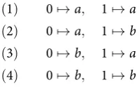
(1) 07→a, 17→a
(2) 07→a, 17→b
(3) 07→b, 17→a
(4) 07→b, 17→b
In this scenario there are 4 meanings (▲,▲,■,■) and 44 = 256 ways to map four
meanings to four signals{aa,ab,ba,bb}. This gives 256 languages of which 4 compo-sitional and 252 holistic.
Not all languages are equally likely. A hierarchical prior that puts a fractionαof the probability mass on the compositional languages:
p(θ) =
{
α
4 ifθis compositional
1−α
256 otherwise
(2.3)
Once an languageθhas been fixed, the agent is presented with new meaningmfor
which it then produces a signalsby sampling from the distribution
p(s|m,z) =
{
1−ε ifm7→sin languageθ
ε/3 otherwise (2.4)
This means the agent will pick the signalscorresponding tomunder languageθmost
of the time, but has a small probabilityεof making an error and uniformly picking
one of the other signals. Together with a completely independent distributionp(m),
typically a uniform one, this specifies the production algorithm
ppa(x|θ) =p(s|m,θ)·p(m), x= (m,s) (2.5)
If x = ((m1,s1), . . .(mb,sb))is the list of the utterances produced by the previous agent, then the posterior distribution is
p(θ|x)∝p(θ)·
b
∏
i=1
ppa(xi|θ), (2.6)
[image:20.595.305.405.238.300.2]and, as usual, the language algorithm takes the formpla(θ|x)∝p(θ|x)η.
2.3. Convergence to the prior
' ' ' '
, %
7QEPPFSXXPIRIGOF!
' ' ' '
, &
1IHMYQFSXXPIRIGOF!
0ERKYWIHMRIZIV]KIRIVEXMSR
' ' ' '
, '0EVKIFSXXPIRIGOF!
X X X X X X
6IPJVIUSJPERKYEKIFIJSVIX
F . Emergence of compo-sitionality in the Bayesian iterated learning model of Griffiths and Kalish ( ). On the left, the lan-guage used in every generation with H one of holistic languages and C – the compositional languages. On the right the relative frequency of every language up to a certain timet. These relative frequencies converge to the prior (orange). Larger bottlenecks (subfigures A–C) slow down convergence.
WebPPL simulation with
α=0.5,ε=0.001and samplers (η=1).
to be used much more frequently, which is confirmed by the plots on the right. There
we see the relative frequency of every language up to several pointstin the simulation.
These plots indicate that the relative frequencies converge to the prior, shown in or-ange. Since the compositional languages have a higher prior probability than each of the holistic languages, they are more frequent. The convergence rate towards the prior
is much faster when the bottleneck is small (b =1, subfigure A) than when it is large
(b =10, subfigure C). It is clear why this happens: the more data is transmitted, the
greater the probability that the child can reconstruct the language. The result is that languages will be stable throughout multiple generations, as seen from the lines in fig-ure 2.3c. Nevertheless, even with a large bottleneck the relative frequencies seem to converge to the prior, be it very slowly. We will discuss all these findings in more detail later. First, what discuss the observed ‘convergence to the prior’.
Convergence to the prior
Let me briefly summarise what we have seen so far. Bayesian agents observe utterances
xt−1produced by the previous agent, and then use Bayes’ rule to infer a language. This
language isθis drawn frompη(θt|xt−1) =p(θt|=x)η, whereηinterpolates between
a sampling- and map-strategy forη=1 andη=∞respectively. All this results in a
chain of the form
x0−→θ1−→x1−→θ2−→x2· · ·. (2.7)
Griffiths and Kalish (2005) noted that several Markov chains can be discerned in eq. 2.7, of which the long-term behaviour is well-studied: They often converge to a so called sta-tionary distribution. This characterised the long-term behaviour of the iterated learn-ing model.
Appendix A introduces the relevant convergence results for Markov Chains; I only
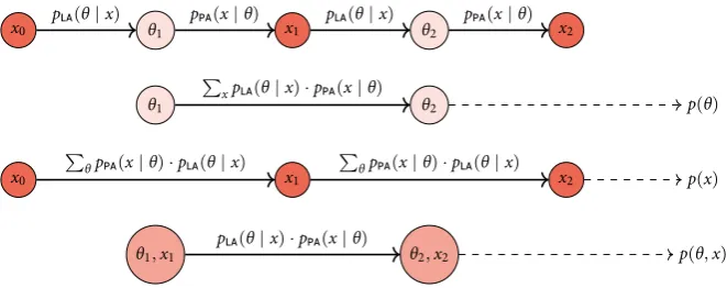
vari-F . Different Markov chains hidden in the Bayesian iterated learning model, and to which sta-tionary distribution they converge (right).
Figure adapted from Griffiths and Kalish ( ).
x0 θ1 x1 θ2 x2
p (θ|x) p (x|θ) p (θ|x) p (x|θ)
θ1 θ2 p(θ)
∑
xp (θ|x)·p (x|θ)
x0 x1 x2 p(x)
∑
θp (x|θ)·p (θ|x)
∑
θp (x|θ)·p (θ|x)
θ1,x1 θ2,x2 p(θ,x)
p (θ|x)·p (x|θ)
ablesx0,x1,x2, . . . indicate the state at every time step, they form a Markov chain
if the probability of moving to another state only depends on the last state: p(xt |
x0, . . . ,xt−1) = p(xt | xt−1). If the number of states is finite, thesetransition
prob-abilitiescan be collected in the transition matrixT. Suppose the initial distribution over states is given by vectorπ, then the next distribution isp(x1 = i) = (Tπ)iand
aftertsteps,p(xt = i) = (Ttπ)i. These probabilities can converge to the so called stationary distributionπ⋆which must be an eigenvector ofTsinceTπ⋆ = π⋆. If the
Markov chain isergodicit is guaranteed to have a unique stationary distribution to
which it converges: p(xt =i) → π⋆
i ast → ∞. Ergodicity, briefly, ensures that the
chain keeps revisiting the entire state space and has a positive probability of reaching any other state from any given state in a finite number of steps. How often it visits every state is given by the stationary distribution, in the sense that the relative frequencies of visited states converges to the stationary distribution.
Griffiths and Kalish (2005) noted that by
marginalising out the productionsxtin eq. 2.7 one obtains the following Markov chain
(see also figure 2.4):
p(θt|θt−1) =
∑
xt−1
pla(θt|xt−1)·ppa(xt−1|θt−1). (2.8)
We hitherto assumed that the transition probabilities remain constant over time, that is, we looked at time-homogeneous chains. The Markov chain in eq. 2.8 is only homo-geneous if all agents use the same production and language algorithms. In particular, they should all use the same prior. We will later discuss the validity of this
assump-tion. If these assumptions hold and the chain is moreover ergodic,thenthe long-term
behaviour of iterated learning is known: convergence to the stationary distribution, independent of the initial distribution.
The stationary distributionπ⋆of this distribution happens to be the priorq(θ) :=
p(θ). To show this, one has to see that
q(θt+1) =
∑
θt
p(θt+1|θt)·q(θt) (2.9)
I have writtenqfor the prior to highlight that we do not know whetherq(θt+1)is a
Oth-2.3. Convergence to the prior
erwise, the following derivation shows that eq. 2.9 holds:
∑
θt
q(θt)·p(θt+1|θt) =
∑
θt
q(θt)·∑
xt
pla(θt+1|xt)·ppa(xt|θt) (2.10)
=∑
xt
pla(θt+1|xt)·
∑
θt
q(θt)·ppa(xt|θt) (2.11)
=∑
xt
pla(θt+1|xt)·ppa(xt)
(⋆)
= ∑
xt
ppa(xt|θt+1)·q(θt+1)
ppa(xt) ·
ppa(xt)
=q(θt+1)
∑
xt
ppa(xt|θt+1)
=q(θt+1)
where(⋆)holds by definition ofpla(θt+1 |xt)and because we use samplers (η=1). For maximisers, the proof breaks down at this point.
Similar results hold for the other Markov chains hidden in the iterated learning model (see figure 2.4). When averaging over interpretations rather than productions, one obtains a Markov chain on the productions:
p(xt+1|xt) =
∑
θt+1
p(xt+1|θt+1)·p(θt+1|xt). (2.12)
A proof analogous to eq. 2.10 shows that this chain converges to theprior predictive
distribution p(x) =∑θppa(x|θ)·p(θ)Finally, one could consider a Markov chain over the state space of language-utterance pairs(θ,x)∈Θ× Xwith transition probabilities
p(θt+1,xt+1|θt,xt) =p(θt+1|xt)·p(xt|θt). (2.13)
This chain has the jointp(θ,x) =ppa(x|θ)·p(θ)as its stationary distribution.
Inter-estingly, this shows that Bayesian iterated learning implements aGibbs sampler.
Gibbs samplers are often used in Bayesian statistics, whenever it is not possible to
work with complicated distributions analytically.Monte Carlo methodsare work-arounds
that collect many samples from the distribution, and approximate the distribution us-ing those samples. To obtain samples, one constructs a Markov chain whose stationary distribution is the distribution of interest. Over time, the visited states will be
(corre-lated) samples from the target distribution. This is the basic idea behind manyMarkov
Chain Monte Carlo(mcmc) methods and Gibbs sampling is one of those. It can be used to approximate a joint distributionp(θ,x)if it is easy to sample from the conditional distributionsp(θ |x)andp(x|θ). In every iteration, it fixes one of the variables, say
θtand samples a newxt+1fromp(xt+1 | θt). Then it fixesxtand samplesθt+1from
? What kind of behaviour should one expect in populations of maximisers? This turns out to be a much harder question. There are, to the best of my knowledge, two analytical results — we will return to em-pirical evaluations in chapter 4 — both suggesting that in populations of maximisers the behaviour is largely determined by the prior, but in a less direct way. First of all, Kirby, Dowman, and Griffiths (2007) analyses the stationary distribution for
maximis-ers (η>1) using a constrained set of languages that spread the probability mass
uni-formly over a (sub)set of utterances.4
This constraint on languages has a purely mathematical mo-tivation: it is precisely what is needed to factorise the normalis-ing constant in the posterior.
In other words,p(x | θ)is either 0 or equal to af(x), where the latter does not depend onθ. In that case, the stationary distribution is proportional top(z)η. This implies that cultural evolution results in an exaggerated version of the prior (cf. figure 2.2).
A similar conclusion follows from the second result, due to Griffiths and Kalish
(2007). They note that maximisers (nowη = ∞) implement a version
Expectation-Maximisation(em). This is an iterative algorithm used in models with hidden vari-ables to estimate parameters that are increasingly close to the maximum likelihood estimates, or, in our case, map estimates. The trick is to use the current parameters to
estimate theexpectedlikelihood of the observed and hidden variables, and then update
the parameters so that theymaximizethat likelihood. When computing the
expecta-tion analytically is intractible, it can be approximated by drawing several samples. The
case using a single sample is calledstochastic em. Now, suppose, in em jargon, there
are no observed variables,xtis the latent variable andθtthe parameter, then stochastic
em in this model amounts to Bayesian iterated learning in a population of maximisers (see Griffiths and Kalish (2007) for details). This characterisation is not as clear-cut as with samplers, but suggests that the stationary distribution over languages will roughly be centred on the maxima of the prior (Griffiths and Kalish 2007).
Convergent controversy
Theconvergence to the priorwas the first general result about the long-term behaviour of the iterated learning model. For populations of samplers, the result was crystal clear: starting from any initial distribution, the probability that an agent down the chain would be using languageθis given by the prior probabilityp(θ). And this is precisely what we observed in figure 2.3, which shows the the emergence of compositionality — or rather, the emergence of the prior. The model is an ergodic Markov chain, and over time the probability that a certain language will be used therefore converges to its prob-ability under the stationary distribution, which is the prior. Compositional languages have high probability under that prior, and consequently emerge. Maximisers are much harder to analyse. The probability that a language is used by maximisers seems to be largely determined by the maxima of the prior. Now, what are the implications of all this for cultural language evolution?
2.4. Convergent controversy
Griffiths and Kalish (2007) conclude that “the emergence of languages with particular properties does not require a bottleneck” (p. 466). Larger bottlenecks do slow down convergence since they imply more faithful transmission and this increases language stability. The Markov chain’s walk through the state space consequently slows down, which, somewhat paradoxically, also slows down convergence. But in the long run bot-tlenecks play no role — at least for samplers. This seems to undermine the idea that
compressible languages emergebecause of cultural transmission. Should we conclude,
then, that languages are not shaped by cultural evolution, but primarily by innate con-straints? Griffiths and Kalish (2007) conclude that their results “do not indicate which of these explanations is more plausible” (p. 475). There’s something for everyone: if the prior captures innate biases, “iterated learning acts as an engine by which these constraints result in universals” (p. 475), but if you prefer the transmission process to actually change the priors, then you “can take heart from our results for learners who use map estimation”.
Kirby, Dowman, and Griffiths (2007) follow the latter advise. Their paper discusses an iterated learning model with maximisers that have a prior bias towards regular lan-guages. Bottleneck effects can occur in populations of maximisers (Griffiths and Kalish 2007) and the authors accordingly conclude that as the bottleneck tightens in their model, “regularity is increasingly favoured”. But there is something peculiar about this conclusion: It seems to hold only because their prior favoured regularity. Had their prior favoured irregularity, irregularity would have been increasingly favoured under a tighter bottleneck.5
I found their paper is a bit sketchy on the details of their simulations, but these conclu-sions follow directly from Grif-fiths and Kalish ( ) and as far as I can see apply equally to Kirby, Dowman, and Griffiths
( ).
In the Bayesian model, transmission at most amplifies pre-existing biases, which of course can be seen as an effect of cultural transmission. Another con-clusion of Kirby, Dowman, and Griffiths (2007) is therefore that processes of cultural
evolution can “completely obscure” thestrengthof the bias. A small tendency to favour
languages with higher prior probability (i.e.η>1) amplifies weak biases and results
in strong universals. The strength of the bias has no role, only the ordering of the lan-guages. All in all, it suggests a rather toothless process of cultural evolution. Several researchers therefore started tweaking the assumptions of the model to find out how robust the results are.
The population structure was one of the first things addressed. It should be noted that (Griffiths and Kalish 2007) gen-eralised their findings to somewhat different scenario, with finite generations evolving in (discrete or) continuous time (cf. Nowak, Komarova, and Niyogi 2001). In that case theproportion pt(θ)of the population speaking languageθat timetconverges to the priorp(θ), as can easily be seen. Ifpt = (pt(θ) :θ ∈Θ)andTthe transition matrix,
these proportions change as
pt+1=Tpt, (2.14)
an alternative model where agents learn from a mixture of the languages used in the previous generation, not just one. This leads to markedly different nonlinear behaviour with bifurcations and possibility multiple equilibria, which they argue accurately de-scribes historical developments (namely, that English is no longer a ‘verb-second’ lan-guage).
That the behaviour changes in different populations structures was confirmed in several other studies. Smith (2009) similarly considered infinite generations of agents learning from multiple parents. He reports that this precludes convergence to the prior and introduces a dependency on the initial distribution of languages in the population. Ferdinand and Zuidema (2009) draw the same conclusion, but also drop the assump-tion that all agents share the same innate biases, i.e. that the populaassump-tion ishomogeneous. In heterogeneous population the convergence to the prior breaks down. Dediu (2009) finds that the strong differences between samplers and maximisers disappears in pop-ulations with a different structure or heterogeneity.
The agents in studies such as Ferdinand and Zuidema (2009) are not Bayesian agents in the strict sense that agents assume to be learning from a single language, while in fact the data comes from several sources. Burkett and Griffiths (2010) address this issue in a hierarchical model where agents take into account that they are possibly learning from multiple languages. Accordingly, the convergence to the prior reappears. Very recently, Whalen and Griffiths (2017) extended this to populations with arbitrary net-work structures, although it should be stressed that agents still learned from a single teacher. Nevertheless, the emerging consensus appears to be that in slightly more com-plicated population structures (with possibly imperfect Bayesian reasoners) the con-vergence to the prior can break down and nontrivial cultural effects appear.
It is somewhat surprising that the pop-ulation structure received most criticism, since that aspect of the Bayesian model is perfectly in line with the original iterated learning model. Some other parts, I would argue, are not. First of all, the type of convergence — in language or in probability of using a language — is markedly different. In early iterated learning studies, the popu-lation converged to a stable language which could be transmitted faithfully along many generations. In the Bayesian models, nothing of this sort happens. In the simulation of the emergence of compositionality (figure 2.3) one clearly sees that successive gen-erations can acquire radically different languages: picture English-speaking parents, themselves born to Basque parents, whose children miraculously learned Hungarian.
Transmission in the Bayesian model generally not faithful — indeed, this is neces-sary for ‘convergence’ to occur at all. That seems particularly problematic for a model of cultural evolution. Even if transmission shapes languages, it has to be somewhat
faithful if one expects any kind of culturalevolution. Tomasello (1999) points out that
faithful transmission is important because it enables a so calledcultural ratchet, where
cultural innovations are passed on and improved upon by later generations. Cultural
evolution, as a result, iscumulativeand products of cultural evolution consequently
infi-2.5. Conclusions
nite reinvention of the wheel — pretty much the exact opposite of cumulative cultural evolution.
Conclusions
The first iterated learning models suggested that languages primarily pick up system-aticity during cultural transmission. Simulations showed how compositional structure accumulated in initially unstructured languages when a bottleneck pressured the lan-guages to become more compressible. However, the learning algorithms that generalise a few observations to a full language implement all kinds of implicit biases, and pos-sibly provide an implicit pressure towards compositional structures. To make general claims about the interaction of cultural processes and innate biases, the two need to be separated clearly. Bayesian iterated learning models did precisely that, but were also
shown toconverge to the prior. That meant that the probability that a certain language
would be used, is after a while completely determined by the biases of the learners, in-dependent of the initial conditions. In populations of maximisers, the relation is less transparent and the shape of the prior (its maxima in particular) largely appears to determine the outcome of cultural evolution.
The Bayesian iterated learning model moved the explanatory load from the cultural process to the prior biases of the learners. However, the strong conclusions were in several studies shown to break down in more complicated populations. The Bayesian model moreover results in an arguably unrealistic model of cultural evolution, with no language stability, nor any cumulative effects. Despite these shortcomings, the field made significant progress due to the work of Griffiths and Kalish. Explicitly encod-ing the biases of the learners made studies of the interactions between the ‘nature’ and ‘nurture’ of language much more principled, and moreover resulted in cognitively bet-ter motivated agents. The focus on analytic results regarding the long-bet-term behaviour brought further transparency to the somewhat opaque conclusions suggested by sim-ulations alone — irrespective of whether the results are ultimately convincing.
In sum, combining the criticism and benefits, I would draw up the following list of desiderata for a model that aims to show that cultural processes can shape the evolution of language (in arbitrary order):
(d1) Explicate biases. The biases of the agents should be explicitly specified in the
model.
(d2) Strategies.The model should explore a wide range of strategies, such as sampling
or map strategies.
(d3) Analysable.The model should be amenable to analytical scrutiny, and it should
ideally be possible to draw general conclusions about long-term behaviour.
(d4) Nontrivial cultural effects.The model should exhibit non-trivial cultural effects,
which might for example result in lineage-specific evolution: different runs re-sulting in different outcomes of cultural evolution.
(d5) Robustness to population structure. The model should exhibit behaviour that
(d6) Language stability.The model should result in a ‘reasonable’ degree of language stability. Reasonable, since languages are never perfectly stable (see also Kirby 2001).
(d7) Empirically testable.The model should give an empirically plausible,
mechanis-tic explanation of cultural evolution, which is further testable against empirical linguistic findings (predating the lab).
Naming
Games
How can a population negotiate a shared language without central
coor-dination? This is the terrain of naming games, the second class of
agent-based models. In local, horizontal interactions, agents ’align’ their
lan-guage until they reach coherence. We discuss several alignment
strate-gies, some of which return in later chapters, and conclude with a proof
suggesting that a stable, single-word language always emerges. The model
used therein is the stepping stone for the next chapter, where we connect
naming games to Bayesian models of iterated learning.
. . The basic naming game . . . 30
. . The minimal strategy . . . 31
. . Lateral inhibition strategies . . . 34
. . Proof of convergence . . . 35
Naming games(ng) or language games were pioneered in the 90s by Luc Steels and colleagues. The view of language that motivated their work was similar to the views expressed in the iterated learning literature. As Steels (1995) puts it, “language is an autonomous adaptive system, which forms itself in a self-organising process”. How-ever, language games approach the adaptive system from a different angle than iterated learning. The development of linguistic structure is not primarily driven by
transmis-sion, as Kirby and others proposed, but “by the need to optimisecommunicative
suc-cess” (p. 319, my italics). The central question takes the form (Steels 2011): how can
a convention of some sort (lexical, grammatical, or otherwise) emerge in and spread through a population as a result of local communicative interactions, that is, without
central coordination? So if iterated learning is a model ofverticallanguage evolution,
then the naming games modelhorizontallanguage evolution.
One of the first studies to explore this, Steels (1995), used a game in which (software) agents negotiated a spatial vocabulary. Equipped with a primitive perceptual appara-tus, the agents learned to identify each other by name or spatial position in a shared simulated environment. Later research extended this approach to embodied robotic
agents, grounding their ‘language’ in the physical world. Thesegrounded naming games
(Steels 2012; Steels 2015) introduce additional complexities pertaining to the percep-tual and motor systems of the robots. We focus on non-grounded games, which can
be divided into two branches. The first is centred around theminimal naming game,
studied extensively using methods from statistical physics. The second extended the first naming games to more complex and possibly realistic linguistic scenarios. This chapter discusses and compares both branches. Of particular interest is the kind of dynamics one can expect from these models. We therefore conclude with the proof by De Vylder and Tuyls (2006) suggesting that naming games always converge to a stable, single-word language.
The basic naming game
Picture a group of people encountering a colourless green object for which they do not have a name. Of even worse, suppose they don’t have a shared language at all. Confused, I suppose, they furiously shout out names for the object. But can they gradually align their vocabularies by carefully attending to what the others are saying, until they have
agreed on a word for the object —gavagai, perhaps?
Frivolities aside, this is the essence of the naming game. It imagines a population of
Nagents in a shared environment filled with objects, which the agents try to name. At
the start of the game, there is no agreement whatsoever about the names of the objects. Every agent has an inventory of names for the objects (a lexicon), which is adjusted after every round with the goal of increasing communicative success. In every round, two randomly selected agents interact, one as speaker, one as the hearer, according to the following script (Wellens 2012):
1. The speaker selects one of the objects which is to serve as thetopicof the interac-tion. She6
‘Gender’ is only introduced to convieniently disambiguate the intended agent: thespeaker (she) or thehearer (he). This even puts the ‘men’ in the role of listener — which I belief is sometimes regarded to be the appropriate role.
3.2. The minimal strategy
A.Failed communication
=⇒
Gavagai Spam Gavagai Spam
Cofveve Foo Cofveve Foo
Spam Spam Gavagai
B.Successful communication
=⇒
Gavagai Spam Spam Spam
Cofveve Foo Spam
F . The updates of the min-imal naming game illustrated. If communication fails, the hearer adds the word uttered by the speaker (bold) to its vocabulary. After a success, both empty their vocabularies and keep only the communicated word.
Figure inspired by Wellens ( ).
2. The hearer receives the word, interprets it and points to the object he believes was intended.
3. The speaker indicates whether she agrees or disagrees, in that way signalling whether communication was successful.
4. Both the speaker and hearer can update their inventories.
The script is a broad outline and concrete implementations are more specific. How, for example, does the speaker select a word in step 1? The typical assumption is that the speaker uses her own experience as a proxy of the hearer’s inventory and opts for
a signal she would likely interpret correctly herself. This is a so calledobverter
strat-egy (Oliphant and Batali 1996). Or more importantly, how do the speaker and hearer update their lexicons after the encounter? Here, the sky is the limit. Does the speaker update her lexicon, or the hearer, or both? What happens after successful communica-tions, what after failure? In years of research, one particular script emerged, which is discussed below. It also became clear that whichever update strategy is used, it must
im-prove thealignmentbetween the lexicons Steels (2011). That means that the
probabil-ity that a future encounter will be successful is increased. Such strategies thus reinforce successfully communicated words and this often installs a winner-takes all dynamics which, in the end, leads to a (unique) shared convention. This is best seen in the so
calledminimal naming game.
The minimal strategy
Theminimal naming gamewas introduced by statistical physicist Andrea Baronchelli (2006) and simplifies earlier naming game in several respects (Baronchelli, Felici, et al. 2006). First, it assumes that homonymy cannot occur. Homonymy can only be
intro-duced when a speaker invents anewword for an object that happens to have been used
already to name another object. If the space of possible new words is large enough, we can safely assume that invented words are unique and homonymy will be absent. Sec-ondly, one can assume, without loss of generality, that there is only one object. If there is no homonymy, the update in step 4 will never affect words used for a different object. The competition between the synonyms for a particular object is thus completely inde-pendent from other objects. As a result, the dynamics of a naming game with multiple objects is fully determined by the dynamics of a game with a single object.
step 4 distinguishes two cases.
• Success.If the hearer knows the word, communication is successful. Both hearer
and speaker remove allotherwords from their inventories, yielding two perfectly
aligned inventories with one single word.
• Failure. If the hearer does not know the word, communication fails and the
hearer adds the word to his lexicon.
Figure 3.1 illustrates how the inventories of agents change after failed and successful communication. The dynamics of the games can be studied by collecting several statis-tics (cf. Baronchelli 2017; Wellens 2012), typically with a certain resolution (e.g. after every 10 rounds). Concretely, we measure the following:
• (Probability of) communicative successps(t). The probability that an
interac-tion at timetis successful. These probabilities are estimated by averaging this
binary variable over many runs.
• Total word countNtotal(t)The total number of words used in the population at
timet. Some authors prefer to divide it by the population size to get the average
number of words per agent.
• Unique word countNunique(t).The number of unique words used in the
popu-lation at timet.
Due to the stochasticity of the games, individual runs vary substantially and can ob-scure underlying regularities. Conversely, the behaviour of a single run can suggest regularities that do not generalise. For that reason, we study the average behaviour of the games, obtained by averaging over many simulation runs.
The minimal naming game goes through three distinct phases, as illustrated in figure 3.2. In the first phase, most interacting agents will have empty vocabularies and thus invent new words. This results in a sharp increase of the number
of unique wordsNunique in the population. In the second phase, no new words are
invented, but the invented words spread through the population. Alignment is still low
and words will rare rarely be eliminated, soNtotalkeeps growing. In the third phase,
after the peak ofNtotal, this changes. Interactions are increasingly likely to be successful,
leading to a sharp increase in communicative success and a drop inNtotalas more and
more words are eliminated. This also results in the characteristic S-shaped curve of
psuccess. Eventually the population reaches coherence in the absorbing state where all
agents share one unique word and reach perfect communicative success (Nunique =1,
Ntotal=Nandpsuccess =1).
The game has two important properties, that one might calleffectivenessand
effi-ciency. The resulting communication system iseffectivebecause agents learn to
com-municate successfully, and efficientin the sense that agents do not memorise more
words than strictly necessary (one, in this case). A simple argument shows that the minimal naming game almost always reaches an efficient and effective stable state (Baronchelli, Felici, et al. 2006). At any point in the game, there is a positive probability of reaching
coherence in 2(N−1)steps: pick one speaker and let her speak to all otherN−1
agents twice. The first time, a hearer might still have to adopt the word, but after the
3.2. The minimal strategy
%
9RMUYIERHXSXEP[SVHGSYRX
2YRMUIX
2XSXEPX
&
'SQQYRMGEXMZIWYGGIWW F . The dynamics of the
minimal naming game. An sharp transition leads to convergence and the emergence of consensus.
Results shown forN=200; avg. of runs, std. shaded.
of this (unlikely) sequence of interactions, the probability that it has not occurred af-terk·2(N−1)steps is less than(1−p)k, which decreases exponentially ink. With
probability 1, the population will thus reach coherence ask → ∞. The argument is
somewhat unsatisfactory as it does not reveal anything about the dynamics: how fast is the convergence, for example?
To obtain a better insight in the dynam-ics, one can adopt a methodology commonly used in statistical physics and look at
scaling relations. The question is then how certain quantities, like convergence time,
scalewith the size of the system, i.e. the number of agents. To that end, two critical
points are identified: the timetconv where the game reaches coherence and the time
tmaxat which pointNtotal(t)reaches its maximum. It turns out that these quantities
de-pend on the population sizeNin a power-law fashion (Baronchelli, Felici, et al. 2006;
Loreto et al. 2011):
tconv, tmax, Ntotal(tmax)∝Nα whereα≈1.5 (3.1)
Now note thatNtotal(tmax)/Nis the maximum number of words each agent has to store
on average — the maximum memory load, perhaps. Baronchelli (2017) concludes that
“the cognitive effort an agent has to take, in terms of maximum inventory size,depends
on the system sizeand, in particular, diverges as the population gets larger” (Baronchelli 2017, italics in original). Although interesting, I would be hesitant to concede that linguistic activity in a small language community requires less cognitive effort than the same activity in a larger community.
Besides the scaling effects, the role of the network structure of the population has been studied extensively (see Baronchelli 2017, for an overview). In the classical
nam-ing game any two agents can interact — there ishomogeneous mixing—
T . Parameter settings for four different strategies, whose be-haviour is shown in figure . . Note that equivalent parametrisations also exist; see main text for details.
δinc δinh δdec sinit smax
1
. ∞
. . . 1
. . . 1
∞
Lateral inhibition strategies
The minimal strategy is somewhat opportunistic in that it forgets all other words after a successful encounter. It has been suggested that subtler alignment mechanisms might
yield faster convergence times: so calledlateral inhibition strategies(see Wellens 2012
ch. 2, for an overview). The name is ultimately derived from biology, where excited
neurons can be found to inhibitneighbouring neurons. Similarly, lateral inhibition
strategies decrease the chance of using competing words again. To that end, they assign ascoreto every word. If a word is communicated successfully, its score is increased, and
the scores of competitors are decreased orinhibited. The production mechanism must
also accounts for the scores, typically by producing the highest-scoring word.
The (basic) lateral inhibition strategy was first formulated in Steels and Belpaeme
(2005) and is described by five nonnegative parameters (Wellens 2012)7
Wellens ( ) only usesδ’s in (0,1), but this general formula-tion allows the inclusion of the frequency strategy.
δinc, δinh, δdec, sinit, smax. (3.2)
After a success, both agents increase the score of the communicated word byδincand
decrease scores of competitors byδinh. After a failure, the hearer adopts the word with
scoresinitand the speaker decreases the score byδdec. Whenever a score drops below
(or equals) 0 the word is removed, and scores can never grow larger thansmax. Other
inhibition strategies have also been used and will be discussed in chapter 7.
The minimal strategy is a special case of the lateral inhibition strategy, forδinc =
δdec=0 andδinh=sinit=1 (see also table 3.1). With those parameters new words get
score 1 and this score is never further increased. Itcanbe inhibited, by 1, which leads
to to immediate removal. In this strategy, the scores thus play a purely administrative
role. A strategy where scores play a larger role, is thefrequency strategywhich counts
how often every word has been encountered. This strategy however exhibits no form of lateral inhibition. The minimal strategy and frequency strategy thus mark two ex-tremes: the former has the strongest possible form of lateral inhibition, the latter none. Between these endpoints lie the proper lateral inhibition strategies.
I want to discuss three fairly different li strategies here: li strategy 1 is a strategy that returns in chapter 6; strategy 2 is taken from Wellens (2012); and strategy 3 is a varia-tion thereof. The parameters are listed in table 3.1 and figure 3.3 shows the dynamics. First of all note that the dynamics ofNuniquecan strongly differ for different strategies
(subfigure a). If for example δinh = δdec as in li strategy 3, many more words can