Intuitionistic implication without disjunction
Gerard R. Renardel de Lavalette Lex Hendriks
Dick de Jongh
July 12, 2010
Abstract
We investigate fragments of intuitionistic propositional logic containing implication but not disjunction. These fragments are finite, but their size grows superexponentially with the number of generators. Exact models are used to characterize the fragments.
1
Introduction
Intuitionistic propositional logicIpL, envisaged as the free Heyting algebra over a nonempty collection of generators P, is infinite. When P is a singleton, we obtain the well-known Rieger-Nishimura lattice. For largerP, however, the free Heyting algebra is very complex and little is known about it. This is unlike the situation for classical logic: Boolean algebras over finitely many generators are finite, and their structure is well known.
Closer inspection learns that the combination of disjunction and implication causes the free Heyting algebras to become infinite. When we only consider formulae ofIpLwithout disjunction, the corresponding algebras are finite; idem if we drop implication instead of disjunction.
In this paper, we investigate fragments of IpL, i.e. sublogics defined by restricting the set of atomic formulae and the set of connectives. We focus on several fragments that contain → and not ∨: see Fig. 1 (observe that we treat double negation ¬¬as a connective on its own).
We denote a fragment by listing the generators and connectives between square brackets, so [p, q,∧,→] is the fragment consisting of formulae that only contain the propositional variables p, q and the connectives ∧ and →. When the identity of the propositional variables is not relevant but only their number, we may write e.g. [∧,→]n for the fragment withnpropositional variables.
The diagram F≡ of fragment F is the set of the equivalence classes of its
formulae, partially ordered by the derivability relation. Some small diagrams are drawn in Fig. 2. We shall see that the size of these diagrams grows super-exponentially with the number of generators.
We shall use exact and quasi-exact models to study the diagrams of frag-ments. A finite model M = hW,6,atomi is an exact model for fragment L
[¬,∧,→]
[¬,→] [¬¬,∧,→]
[¬¬,→] [∧,→]
[image:2.595.218.377.100.242.2][→]
Figure 1: Inclusion diagram of the fragments studied in this paper.
p→p
¬¬p ¬¬p→p
p ¬p
¬(p→p)
pp
qpqq pqqpp pqpp
qp pqq pqpp∧qpqq qpp pq
pqp pqqp pqq∧qpp qppq qpq
p pq∧qp q
p∧q
Figure 2: The diagrams of [p,¬,∧,→] and [p, q,∧,→]. To reduce the size of formulae, the implication arrows are omitted in the right hand diagram: so e.g.pqpabbreviates (p→q)→p.
subsets ofW. So an exact model is also a minimal universal model: it is (mod-ulo isomorphism) the smallest model such that equivalence in the model implies provable equivalence in the fragment. As we shall see, from the fragments con-sidered here only the fragments [P,¬,∧,→] and [P,∧,→] have exact models. Other fragments will be characterized byquasi-exact models, where the diagram
F≡ is not isomorphic with the full ℘u(W), but only with a subset of it.
1.1 The historical perspective
[image:2.595.116.410.290.484.2]As a forerunner, one may consider Th. Skolem’s 1919 paper [35] on the application of concepts from (what we now call) lattice theory to non-classical logics. But it really started with A. Heyting’s groundbreaking formalisation [16] of intuitionistic logic in 1930. This led to the notion of Heyting algebras, and to the natural question: what is the structure of the free Heyting algebra, i.e. the algebra of the equivalence classes of formulae of IpL? In 1932 K. G¨odel proved in [12] that this algebra is infinite, in other words: IpLdoes not have a finite set of ‘truth values’. N. Rieger [33] discovered in 1949 that the fragment ofIpLwith only one propositional variable has already infinitely many equivalence classes. This free Heyting algebra over one generator is a nice lattice, rediscovered by I. Nishimura [29] in 1960.
In 1952, Skolem [36] showed that in the intuitionistic algebra of pure im-plication, every formula containing not more than two variables is equivalent to one of a collection of 14 formulas. This diagram of the fragment [→]2 must have been rediscovered many times since (and maybe even before) by several logic students. The same will undoubtedly be true for the 18-point diagram of [∧,→]2 (see Fig. 2), first published by R. Balbes [1] in 1973.
A first systematic study of the algebras corresponding to the [→] and [∧,→] fragments of IpL, calledHilbert algebras1andBrouwerian (orimplicative) semi-lattices respectively, was published by A. Monteiro [27] in 1955.
In 1955, E. Beth developed in [3] a semantics for intuitionistic logic based on semantic tableaus, emerging from systematic attempts to disprove the deriv-ability of a formula (see also [20]). Similar ideas for possible world semantics for modal logic were investigated by S. Kanger and J. Hintikka. These devel-opments culminated in S. Kripke’s famous paper in 1965 on the semantics of intuitionistic logic [22] in terms of partial orders of possible worlds, now known as Kripke models.
In this period, the interest in the connections between logic and (universal) algebra increased, as can be deduced from the popularity of the book The mathematics of metamathematics [31] by H. Rasiowa and R. Sikorski, published in 1963. Several attempts were made to connect the algebraic and the partial order approach to the semantics of IpLand the intermediate logics betweenIpL and classical propositional logic, e.g. in 1966 by Heyting’s and Beth’s students A. Troelstra and one of the authors (De Jongh) in [37].
In 1965 A. Diego, a student of Monteiro, proved in [9] the basic result for the area of our research: finitely generated Hilbert algebras are finite. G. McKay seems to have been the first to observe in 1968 in [26] that Diego’s result can be extended quite easily to implicative semi-lattices. Independently, Urquhart [39] proved the finiteness of the diagrams of [→]n and [∧,→]n in 1974.
Finite implicative semi-lattices are bounded: for all x we have b6x 6⊤, where b = ⊥ if the fragment contains negation and otherwise b = V
P with
P the set of atomic formulae in the fragment. They are also lattices, as can be seen by taking V
{x | a 6 x and b 6 x} for a∨b. Using an early result from Skolem [35], implicative lattices are distributive; and by a well known
1The term Hilbert algebra is also used for unitary algebras, related to Hilbert spaces and
theorem of G. Birkhoff [4], distributive lattices are isomorphic to the lattice of upward closed subsets of the partially ordered set of their (join-)irreducible elements. Based on these insights and Diego’s result, the following question comes up naturally: what is the structure of the underlying partial orders of the diagrams of [→]n, [∧,→]n and [¬,∧,→]n? N. de Bruijn was the first to
address this question in [6] (a shorter version appeared as [8]). He baptised these underlying partial ordersexact models: they turn out to be Kripke models. These exact models are finite, which gives another proof for Diego’s result. De Bruijn discovered the 61-point exact model of [∧,→]3 (see Fig. 7) and used it to compute the size of its diagram: 623 662965 552330. In [7], De Bruijn developed an Algol60 computer program to test formulas in [∧,→]3 based on the exact model. Such programs using model checking are in general much faster than, e.g., tableau-based testers.
Due to their somewhat obscure publication medium, De Bruijn’s results were not immediately noticed in the algebraic or logic communities. Building upon the pioneering work of Rasiowa and Sikorski [31] on algebraic semantics and Nemitz [28] on implicative algebras, Landolt and Whaley [25] and Krzys-tek [23] studied free implicative semilattices and duplicated independently De Bruijn’s results. K¨ohler [21] also studies implicative semilattices, and refers to De Bruijn’s work. He computed the size of the exact model of [∧,→]4 to be 2494 651862 209437, using a formula that improves upon a result in [6] (it is the first formula in Theorem 9 of the present paper).
In the late 1960s, one of the authors (De Jongh) and H. Kamp started the investigation of the structure of the diagrams of fragments of IpL using a tableau-based computer program to compute equivalence classes. Due to the limitations of computer power at that time, only small fragments could be in-vestigated. Later on, De Jongh stimulated one of the authors (Hendriks), H. van Riemsdijk and J. Tromp to continue this research, now using more pow-erful computers. This subsequently led to a research project by the present three authors, focusing on the study of diagrams of fragments of IpL, com-bining tableau-based testers and fast computer programs using exact models, as previously developed by De Bruijn. A first publication of their results is [19], which describes exact models for [∧,→] and [¬,∧,→] as minimal complete Kripke models for these fragments, and provides characteristic formulas for the nodes in exact models, using methods that were developed in De Jongh’s Ph.D. thesis [18] and are akin to those of Jankov in [17]. This research was extended to exact models of [¬,∧,∨] and some subfragments, and resulted in the Ph.D. the-sis of Hendriks [14]. In this thethe-sis, the notion ofsemantic type was introduced, inspired by the notion ofcharacterintroduced in modal logic by K. Fine [10] and G. Boolos [5] (see also [11]). Some of the techniques developed for fragments of IpLhave proved applicable in modal logic and provability logic (see [13]). The computer programs developed by Hendriks were used to find a counterexample for the interpolation property of the fragment [↔]: see [15] and the reference there to [30] by Por¸ebska with an earlier discovery of a counterexample.
algebra over three elements, and refer to [14] for the size of [→]4. In [40], F. Yang studies several fragments of IpL and points out a flaw in the inductive reasoning in proofs of [19] and [14].
The current paper recapitulates the research on fragments of IpL with im-plication and without disjunction in a uniform and perspicuous way; moreover, it introduces new semantical concepts, repairs a flawed proof and presents new results, e.g. the characterisation of fragments with double negation, and the computation of [→]4. In a forthcoming paper, we plan to do the same for the other class of finiteIpL-fragments, viz. those without implication.
1.2 How to obtain exact models
Let us indicate how we will construct exact models of fragments, using the fragment [P,¬,∧,→] as an example.
1. First of all, we need a way to reduce arbitrary (possibly infinite) models to finite models, in a way that is invariant for the formulae in [P,¬,∧,→]. For this, we use the semantical property of inductiveness: a node w in a modelM is inductive iff∀v > w(p∈atom(v)) impliesp∈atom(w), for all propositional variables p∈P. In words: ifp is true in all nodesv above
w, then it is true inw. It appears that this inductive property extends to all formulae ϕin [P,¬,∧,→]: if ∀v > w(v |=ϕ) then w|=ϕ.
2. This suggests that inductive nodes are not needed to distinguish non-equivalent formulae in [P,¬,∧,→]. To make this explicit, we define a reduction operation M−i on models M which eliminates all inductive nodes in M, and we show that all formulae in [P,¬,∧,→] are invariant wrt. this reduction, i.e. M |=ϕ⇔M−i|=ϕfor all ϕ∈[P,¬,∧,→].
3. Furthermore, we identify a ‘maximal’ modelE consisting of only nonin-ductive nodes that containsM−i for everyM. It is not hard to see thatE
is finite, due to the fact that the maximal depth of a node inE is bounded by the cardinality of P. Moreover, we prove: if ϕ, ψ ∈ [P,¬,∧,→] are equivalent in E, then they are equivalent inall models, so E is universal for [P,¬,∧,→].
4. Finally, to show that E is an exact model, we define for every upward closed subsetXinE a formulaϕX in [P,¬,∧,→] that characterisesX in
the sense that we have w∈X ⇔E, w|=ϕX.
For other fragments, we use other semantical properties, based on full and hybrid nodes (Definition 5). For the characterisation of fragments without conjunction, we use the propertyJ(ϕ→ψ)⊆J(ψ) of the semantical mapping
J, first described by De Bruijn in [6].
1.3 Survey of the rest of the paper
studied here. The universal model is presented in Section 4, followed by the definition of exact models as finite submodels of the universal model in Section 5, where we also introduce characteristic formulae and prove the main results about (quasi-)exact models. In Section 6, we have a closer look at the struc-ture of the models and the diagrams, and we derive several formulae about their size and its asymptotic behaviour. The final Section 7 contains some concluding remarks.
For reasons of readability, some proofs are delegated to the Appendix.
2
Preliminaries
Definition 1 (Partial orders and related notions)
Models are constructed as usual from partially ordered setshW,6i, where6is a reflexive, antisymmetric and transitive relation onW. Theone-step order<1 is defined by
v <1 w iffv < w&¬∃u∈W v < u < w.
The cover w of w is the set {v | v >1 w} of one-step successors of w. The
upward closure X↑ ofX ⊆W is defined by
X↑={w| ∃v∈X(w>v)}
and thestrict upward closureX∧is defined asX↑ −X. For closures of singleton sets, we drop the parentheses and writew↑ and w∧. Also
min(X) ={v ∈X| ¬∃w∈X(w < v)}
We adopt analogous definitions for the downward closureX↓, the strict down-ward closure X∨ and for max(X). We say that X, Y ⊆ W are incomparable
if ¬∃x ∈ X∃y ∈ Y(x 6 y∨y 6 x). The depth d(w) of w ∈ W is defined inductively by
d(w) = sup{d(v) + 1|v > w}, where sup(∅) = 0
We put
℘u(W) = {X∈℘(W)| ∀x∈X∀y >x y∈X} ℘a(W) = {A∈℘(W)| ∀ab∈A(a6b⇒a=b)}
so ℘u(W) is the collection of upward closed subsets of W, and ℘a(W) the collection ofantichains, i.e. subsets where no two elements are comparable. We shall use the isomorphism
i:℘u(W)→℘a(W), defined by i(X) =max(W −X) (1)
with inversei−1(A) =W −A↓. iinduces a partial order on ℘a(W), defined by
Definition 2 (IpL and its fragments)
The language ofIpLis defined as usual from propositional variablesp, q, r,· · · ∈
PV, the constant ⊤ and the connectives ¬,∧,∨,→. We shall use P, Q, R, for finite subsets of PV, and we write Pn for the subset {p1, . . . , pn} of PV. ⊥ is defined as¬⊤.
We writeIpL(P) for the collection ofIpL-formulae containing only propositional variables in P ⊆PV. Moreover, when C is a collection of connectives (where we also allow ¬¬ and ⊥), the fragment [P, C] is the collection of IpL-formulae containing as propositional variables only elements ofP and as connectives only elements of C. Since ⊤ is part of the language, IpL(P) and [P, C] are always nonempty, even ifP =C=∅.
Observe that every fragment contains the constant⊤, and that¬and⊥are interchangeable in fragments containing→ (for¬ϕ≡(ϕ→ ⊥) and ⊥ ≡ ¬⊤).
Definition 3 (Models and validity)
A model forP is a tripleM =hW,6,atomiwherehW,6iis a nonempty partial order andatom:W →℘(P) is a mapping that indicates where the propositional variablesp∈P are valid. atomis monotonic, i.e.v6w⇒atom(v)⊆atom(w). We extendatom to sets of nodes byatom(X) =T
{atom(x)|x∈X} ifX6=∅, andatom(∅) =P. In this paper, we only considerlocally finite partially ordered setshW,6i, wherew↑is always finite. MOD(P) denotes the collection of locally finite models for P.
Validity of a formula in a node in a model is defined as usual:
M, w|=p ⇔ w∈V(p)
M, w|=¬ϕ ⇔ ∀v>w(M, v6|=ϕ)
M, w|=ϕ∧ψ ⇔ M, w|=ϕand M, w|=ψ M, w|=ϕ∨ψ ⇔ M, w|=ϕorM, w|=ψ
M, w|=ϕ→ψ ⇔ ∀v>w(M, v|=ϕ⇒M, v|=ψ)
M, w|=ϕ↔ψ ⇔ ∀v>w(M, v|=ϕ⇔M, v|=ψ)
As is well known (see e.g. [38]), we have:
IpLis sound for all models, and complete wrt. the collection of finite models.
An alternative (but equivalent) definition of models uses valuation mappings
V :P →℘u(W) instead of atom. V can be extended to a semantical mapping
V :IpL→℘u(W) by
V(ϕ) ={w∈W |M, w|=ϕ}
When we combine V with the isomorphism i defined in (1), we obtain the mappingJ :IpL→ ℘a(W) with
J(ϕ) =max{w∈W |w6|=ϕ}
So J(ϕ) is the collection of so-called border points that lie outside V(ϕ). The main reason for working with J instead of the more usual mapping V is the property, first mentioned by De Bruijn in [6]:
We shall use this property (which follows from (8) in the next lemma) when we investigate fragments not containing conjunction.
Lemma 1 (Main properties of J)
For all formulaeϕ, ψ we have:
J(p) = {w|p∈atom(w)−atom(w)} (3)
J(⊤) = ∅ (4)
J(⊥) = max(W) (5)
J(¬ϕ) = max(W)−J(ϕ) (6)
J(ϕ∧ψ) = (J(ϕ)∩J(ψ))∪(J(ϕ)−J(ψ)↓)∪(J(ψ)−J(ϕ)↓) (7)
J(ϕ→ψ) = J(ψ)−J(ϕ)↓ (8)
Proof (3), (4) and (5) are verified easily, and (6) follows from (5) and (8). For (7), we reason as follows:
J(ϕ∧ψ) =
max{w|w6|= (ϕ∧ψ)}
=
{w|(w6|=ϕ orw6|=ψ) &∀v > w(v|=ϕ&v |=ψ)}
=
{w|(w6|=ϕ&w6|=ψ&∀v > w(v|=ϕ&v|=ψ)) & (w6|=ϕ&w|=ψ&∀v > w(v|=ϕ))
& (w|=ϕ&w6|=ψ&∀v > w(v|=ψ))}
=
(J(ϕ)∩J(ψ))∪(J(ϕ)−J(ψ)↓)∪(J(ψ)−J(ϕ)↓)
Finally we prove (8).
J(ϕ→ ψ) =
max{w|w6|= (ϕ→ψ)}
=
{w|w6|= (ϕ→ψ) &∀v > w(v|=ϕ⇒v|=ψ)}
=
{w|w|=ϕ&w6|=ψ&∀v > w(v |=ϕ⇒v|=ψ)}
=
{w|w|=ϕ} ∩ {w|w6|=ψ&∀v > w v|=ψ}
=
max{w|w6|=ψ} − {w|w6|=ϕ}
=
J(ψ)−J(ϕ)↓
The following properties ofJ are verified in a similar manner:
J(¬¬ϕ) = max(W)∩J(ϕ) (9)
J(¬¬ϕ→ϕ) = J(ϕ)−max(W) (10)
J((ϕ→ ψ)→ϕ) = J(ϕ)−J(ψ)∨ (11) J((ψ→ϕ)→ϕ) = J(ϕ)∩J(ψ)↓ (12)
J(((ϕ→ψ)→ϕ)→ϕ) = J(ϕ)∩J(ψ)∨ (13)
J(((ϕ→ψ)→ ψ)→ϕ) = J(ϕ)−J(ψ) (14)
J((ϕ↔ ψ)→ϕ) = J(ϕ)∩J(ψ) (15)
J((ψ∧χ)→ϕ) = J(ψ→ϕ)∩J(χ→ϕ) (16)
Definition 4 (Bisimulation)
A relationB between two modelsM =hW,6,atomiand M′ =hW′,6′,atom′i
is abisimulationif it satisfies the following three conditions (where the·denotes relational composition):
B ⊆ {(w, w′)|atom(w) =atom′(w′)}
(>·B) ⊆ (B·>′) (B·6′) ⊆ (6·B)
A functional bisimulation is also called ap-morphism2.
Two elementswandw′ are calledbisimilar if there is a bisimulationBbetween
M andM′ withwBw′. Notation: w↔w′.
Since the union of bisimulations is again a bisimulation, ↔ is the largest bisimulation. We have as a well-known fact, for all formulaeϕ:
if v↔w and v|=ϕ, thenw|=ϕ.
3
Some semantical properties
In this section, we define some semantical properties that are related to the fragments we consider here. First a definition of properties of nodes in a model.
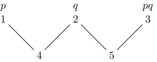
Definition 5 (inductive, full and hybrid nodes) LetM =hW,6,atomi ∈MOD(P) withw∈W.
1. w isinductive or ani-node if it is not maximal andatom(w) =atom(w∧) (i.e. if an atom holds in all worlds above w, then it also holds in w);
2. w isfull or anf-node ifatom(w) =P (i.e. all propositional variables ofP
hold in w);
3. w is hybrid or an h-node if there areu, v withw <1 u,w <1 v, u is full and v is not full (i.e. w has both full and non-full immediate successors).
See Fig. 3 for examples.
We have the following simple properties of inductive and full nodes:
2For modal logic this notion was first invented by K. Segerberg. It was used previously,
1 2 3
4 5
[image:10.595.138.298.108.171.2]p q pq
Figure 3: A model where node 4 is inductive, 3 is full and 5 is hybrid.
Lemma 2
1. Ifϕ∈[¬,∧,→],w inductive and w∧ |=ϕ, then w|=ϕ.
2. Ifϕ∈[P,¬¬,∧,∨,→] and w full, thenw|=ϕ.
The proofs proceed via straightforward induction.
We want to know more about x-nodes (x = f, i or h) than Lemma 2 tells us: what is the class of formulae invariant under the operation of eliminating x-nodes? Therefore we define some reductions of models. InM−f we leave out the full nodes, and in M−i the inductive nodes. In M−h, we do not leave out
nodes but we take away links in the accessibility relation in such a way that hybrid nodes lose their link with full nodes.
Definition 6
LetM =hW,6,atomi ∈MOD(P).
1. M−i =hW−i,6−i,atom−ii, the i-reduct of M, is defined by W−i={w∈
W |wis not inductive}, and6−iandatom−iare the restrictions of6and
atom to W−i.
2. M−f=hW−f,6−f,atom−fi
, thef-reduct ofM, is defined byW−f={w∈ W |wis not full}, and6−fandatom−fare the restrictions of6andatom to W−f.
3. M−h = hW,6−h,atomi, the h-reduct of M, is defined by: 6−h is the reflexive transitive closure of <−1h, where
v <−1hwiff v <1 w& not(v hybrid &w full)
or, equivalently,
v <−1hwiff v <1 w& (atom(w)6=P oratom(v∧) =P)
WhenM contains only full nodes,M−fis empty and hence not a model. In that case, we interpret M−f |= ϕ as vacuously true. For M−i this does not apply,
since every locally finite model has maximal nodes, and they are by definition not inductive.
Lemma 3
For x equals i, f or h, we have
Proof For M−f this is evident. To see that M−i has no inductive nodes: observe that if w were inductive in M−i, then it would also be inductive in
M, so it cannot be in M−i. Finally, M−h has no hybrid nodes, for a hybrid node inM has no full immediate >−h-successors, hence it is no longer hybrid
inM−h.
Now we can define the main semantical properties.
Definition 7 (Invariance)
Let x equal f, i or h. INVx, the collection of x-invariant formulae, is defined by
INVx={ϕ|for all models M : M |=ϕ ⇔ M−x|=ϕ}
Furthermore we define
INVfi=INVf∩INVi
INVhi=INVh∩INVi
VALf ={ϕ|ϕholds in all full nodes }
We writeINVi(P) forINVi∩IpL(P), and similarly for other formula collections.
We shall show that these notions of invariance characterize the fragments con-sidered in this paper. The following theorem is a step in that direction:
Theorem 1
1. INVi contains ⊥and PV, and is closed under¬,∧ and→.
2. INVf contains PV and is closed under∧,∨ and →.
3. INVh∩VALf contains PV and is closed under¬¬,∧,∨ and→.
Proof See the Appendix.
Observe that ⊥ is not f-invariant: if M contains only full nodes, then M−f is empty and by convention M−f |=⊥, while of course M 6|=⊥.
As a direct consequence of Theorem 1, we have one half of the characteri-sation of three fragments:
1. [¬,∧,→]⊆INVi.
2. [∧,→]⊆INVfi.
3. [¬¬,∧,→]⊆INVhi∩VALf.
4
Types and the universal model
Types are objects of the formhP, Xi where P ⊆PV is a collection of proposi-tional variables and X is a finite collection of types. They were introduced as semantic types in [14]. We shall construct models from types as nodes: the first component of a type indicates which propositional variables are valid, and the second components contains its direct successors. So atom(hP, Xi) = P, and the partial order 6 on types is the reflexive transitive closure of the one-step order<1, defined byhP, Xi<1hQ, Yi iffhQ, Yi ∈X.
A collectionXof types is calledclosedwhen we haveY ⊆Xfor allhQ, Yi ∈ X. A closed collection of types X can be seen as a modelhX,6,atomi, where 6and atomare as defined above.
We define the universal model as a collection of types, in such a way that no two types in the universal model are bisimilar. This is realized as follows.
Definition 8 (the universal model)
The universal modelUMof IpL is defined inductively as the smallest collection of types satisfying the following condition:
if X finite and X∈℘a(UM), Q⊆atom(X) and
|X|= 1⇒Q⊂atom(X), thenhQ, Xi ∈UM
Here⊂denotes strict inclusion: X ⊂Y iff X⊆Y and X6=Y.
Observe thathQ,∅i ∈UMfor allQ⊆PV, since∅ ∈℘a(UM) andatom(∅) =PV
(by convention). In general,hQ, Xi is a node inUMifX is a finite antichain in UMwith Q⊆atom(X) and Q is a proper subset of atom(X) in the case that
X is a singleton set. The last condition is added to exclude types of the form
hQ,{hQ, Xi}i inUM, which are bisimilar with hQ, Xi.
In order to embed a locally finite model into the universal model, we define a reduction mapping that maps nodes of the model to types in the universal model.
Definition 9 (reduction mapping)
LetM be a locally finite model: we define the mappingρ=ρM :M →UM.
ρ(w) is defined with induction over the depth of wby
ρ(w) = t ifmin{ρ(v)|v >1 w}={t} and ∀v >1 watom(v) =atom(w) = hatom(w),min{ρ(v)|v >1 w}i otherwise
So ρ(w) = ρ(v) if ρ(v) is the unique element of min{ρ(v) | v >1 w} and atom(w) = atom(v); otherwise ρ(w) = hatom(w), Xi with X = min{ρ(v) | v >1 w}i. It is evident that always atom(w) = atom(ρ(w)), and also that
v6wimplies ρ(v)6ρ(w).
Theorem 2
1. Bisimilar types inUMare equal: ∀st∈UM(s↔t ⇒ s=t).
2. ρM is a bisimilarity (and hence a p-morphism).
3. ρM(w)∈UMfor all models M ∈MODand all winM.
4. UM is a locally finite universal model forIpL, and ρUM is the identity.
Proof See the Appendix.
5
Exact models
In this section we shall define, for finite sets P ⊆ PV, exact models EM¬(P)
for [P,¬,∧,→] and EM(P) for [P,∧,→]. Moreover, we shall define quasi-exact modelsQEM(P) for [P,¬¬,∧,→]. All (quasi-)exact models are finite submodels of the universal model. In the definition, we shall use the modification atomP
ofatom, defined by
atomP(X) =atom(X)∩P,
soatomP(∅) =P, and atomP(X) =atom(X) if X is a nonempty set of nodes
with atoms inP.
Definition 10 (exact and quasi-exact models)
EM(P),EM¬(P) andQEM(P) are defined inductively as follows.
1. IfX∈℘a(EM(P)) andQ⊂atomP(X), thenhQ, Xi ∈EM(P).
2. hP,∅i ∈EM¬(P);
if X∈℘a(EM¬(P)) andQ⊂atomP(X), then hQ, Xi ∈EM¬(P).
3. hP,∅i ∈QEM(P);
if Q⊂P thenhQ,{hP,∅i}i ∈QEM(P);
if X ∈ ℘a(QEM(P) − {hP,∅i}) and Q ⊂ atom
P(X), then hQ, Xi ∈
QEM(P).
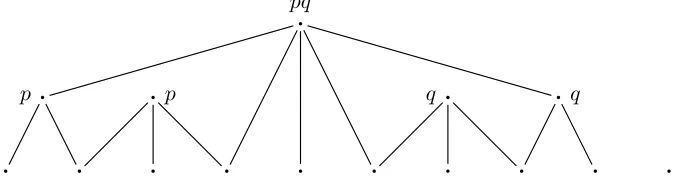
It is evident that EM(∅) = ∅, and that EM¬(∅) = EM({p}) = QEM({p}) = {h∅,∅i}. EM¬({p}) has 3 nodes and equals QEM({p}), and EM({p, q}) has 5
nodes: see Fig. 4. Observe that ℘a(EM¬({p}), the collection of antichains in EM¬({p}), is isomorphic to the diagram of [p,¬,∧,→] given in Fig. 2; idem
for ℘a(EM({p, q}) and [p, q,∧,→]. EM
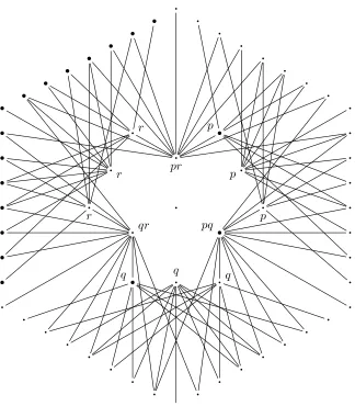
¬({p, q}) has 15 nodes and differs from QEM({p, q}), which has 13 nodes: see Fig. 5 and 6. EM({p, q, r}) with 61 nodes is given in Fig. 7.
We observe that in all these models the nodes with empty atom set are the most frequent, while nodes with larger atom sets are increasingly rare.
In general,EM(P) is a submodel ofQEM(P) which is a submodel ofEM¬(P),
which is a finite submodel ofUM. Moreover, if P ⊆Q thenEM(P)⊆EM(Q), EM¬(P)⊆EM¬(Q) andQEM(P)⊆QEM(Q). We also observe that, in all these
p p q
Figure 4: The exact models EM¬({p}) andEM({p, q})
pq
p p q q
Figure 5: The exact modelEM¬({p, q})
We shall study the structure of these models more closely later on. For now we establish the link between these models and semantical notions introduced earlier.
Theorem 3
1. EM¬(P) is universal forINVi(P)
2. EM(P) is universal forINVfi(P)
3. QEM(P) is universal forINVhi(P)
Proof See the Appendix.
Using the (quasi-)exact models, we define the diagrams of the fragments studied here.
Definition 11 (diagrams)
The diagramsDci(P) (c for conjunction, i for implication),Dnci(P) (n for
nega-tion),Ddci(P) (d for double negation), etc., are defined by
Dci(P) = ℘a(EM(P))
Dnci(P) = ℘a(EM¬(P))
Ddci(P) = ℘a(QEM(P)− {hP,∅i})
Di(P) = Sp∈P ℘(JEM(P)(p)) ⊆ Dci(P)
Dni(P) = Sp∈P ℘(JEM¬(P)(p))∪℘(JEM¬(P)(⊥)) ⊆ Dnci(P)
Ddi(P) = Sp∈P ℘(JQEM(P)(p)) ⊆ Ddci(P)
By Theorems 5 and 8, we have that [P,∧,→]≡ is isomorphically embedded in Dci(P), [P,¬,∧,→]≡ in Dnci(P) to [P,¬,∧,→]≡, etc. In the next section, we
[image:14.595.138.447.611.701.2]pq
[image:15.595.144.405.130.240.2]p p q q
Figure 6: The quasi-exact modelQEM({p, q})
5.1 Characteristic formulae for nodes in exact models
We shall show thatEM(P),EM¬(P) are indeed exact models for [P,∧,→] and
[P,¬,∧,→] respectively, i.e. that for every antichainX in the model there is a formulaψX in the corresponding fragment withJ(ψX) =X. For QEM(P) and
the corresponding fragment [P,¬¬,∧,→], we will do this for almost all upward closed subsets. For this purpose, we define (for E equals EM(P), EM¬(P) or QEM(P)) characteristic formulaeχE,wand prove in Theorem 4 thatJE(χE,w) = {w}.
Definition 12 (Characteristic formulae)
For E = EM(P),EM¬(P) or QEM(P) and w = hQ, Xi ∈ E, we define χE,w
with downward induction over|atom(w)|as follows.
1. E =EM(P). We know that atomP(X)−Q is not empty, so let p be an
element of this set. (We shall see in the proof of Theorem 4 that the specific choice of pdoes not matter.) Now
χE,w= (ϕ1∧ϕ2∧ϕ3∧ϕ4) → p
where
ϕ1 = V
Q
ϕ2 = V{p↔q|q ∈atomP(X)−Q− {p}} ϕ3 = V{(p→χE,x)→p|x∈X}
ϕ4 = V{p→χE,v|v∈Y}
and Y =max{v∈W |v6∈X↑,atom(v)⊇atomP(X)}.
2. E =EM¬(P). As forEM, with the additional casew=hP,∅i, for which
we define χE,w=¬(V
P).
3. E = QEM(P). Here we define χE,w only for w 6= hP,∅i. We proceed as
forEM, with the additional casew=hQ,{hP,∅i}iwithQ⊂P, for which we define (recall that p∈P−Q)
χE,w= (
^
p
p
p
q q
q r
r r
pr
[image:16.595.106.430.101.471.2]pq qr
Figure 7: The exact modelEM({p, q, r}). The fat nodes indicate the embedding of ℘a(EM({p, q})) bye
{p,q,r}, as described in the proof of Lemma 5.
Observe that the definition of ϕ3 is correct, since x ∈ X implies |atom(x)|> |atom(w)|, so χE,x is defined in an earlier stage. Idem for ϕ4, since v ∈ Y implies |atom(v)| >|atom(w)|, and moreover hP,∅i 6∈ Y (which is relevant in the case E = QEM(P)). Observe also that χEM(P),w is indeed a formula in
[P,∧,→],χEM¬(P),w in [P,¬,∧,→] and χQEM(P),w in [P,¬¬,∧,→].
Theorem 4
ForE =EM(P),EM¬(P) or QEM(P) and w=hQ, Xi ∈E, we have
JE(χE,w) ={w}
unlessE=QEM(P) and w=hP,∅i, in which caseχE,w is not defined.
Proof See the Appendix.
Theorem 5
1. [P,¬,∧,→]≡ andDnci(P) are isomorphic.
2. [P,∧,→]≡ and Dci(P) are isomorphic.
3. [P,¬¬,∧,→]≡ andDdci(P) are isomorphic.
Proof 1. We shall show that J =JEM¬(P) : [P,¬,∧,→]→ ℘a(EM¬(P)) is
an isomorphism (recall that Dnci(P) = ℘a(EM¬(P))). J is injective: if ϕ, ψ ∈[P,¬,∧,→] andJ(ϕ) =J(ψ) then ϕ≡ψ, for ϕ, ψ are in INVi(P)
and EM¬(P) is universal wrt.INVi(P). To show thatJ is surjective, too,
let X ∈℘a(E) be arbitrary and defineψX =V
{χE,w |w∈X}: we shall show that J(ψX) = X. By (7), we have that J(ϕ∧ψ) = J(ϕ)∪J(ψ)
whenever J(ϕ) and J(ψ) are incomparable. All different v, w ∈ X are incomparable and J(χE,w) ={w}, so indeedJ(ψX) =S
w∈X{w}=X.
2. Similar.
3. Since℘u(QEM(P)−{hP,∅i}) is isomorphic to{X ∈℘u(QEM(P))| hP,∅i ∈ X}, it suffices for the third part to show that [P,¬¬,∧,→]≡ and {X ∈ ℘u(QEM(P))| hP,∅i ∈X} are isomorphic. Now every ϕ∈[P,¬¬,∧,→] holds in all full nodes, so hP,∅i ∈ VE(ϕ) (where E =QEM(P)). On the
other hand, if X ∈℘u(QEM(P)) and hP,∅i ∈X, then ψ
X is defined and
in [P,¬¬,∧,→]. This proves the last part of the theorem.
So indeedEM¬(P) is an exact model for [P,¬,∧,→],EM(P) for [P,∧,→], and QEM(P) is a quasi-exact model for [P,¬¬,∧,→].
We complete the characterisation of the∧-fragments:
Theorem 6
1. INVi= [¬,∧,→]≡.
2. INVfi= [∧,→]≡.
3. INVhi∩VALf = [¬¬,∧,→]≡.
Proof The inclusions from right to left were formulated as a direct consequence of Theorem 1. For the other direction, we argue as follows.
Let ϕ ∈ INVi∩IpL(P), E = EM¬(P) and X = VE(ϕ). Now ψ = ψX as
defined in the proof of Theorem 5 is a formula in [P,¬,∧,→] that is equivalent with ϕ on EM¬(P), i.e. EM¬(P) |= ϕ ↔ ψ. By Theorem 1, we have that ϕ↔ψis i-invariant, so with Theorem 3 we now get|=ϕ↔ψ, i.e. ϕandψare equivalent.
5.2 Fragments without conjunction
We now look at fragments without conjunction, and introduce two classes of formulae.
Definition 13
DIMPand DNEG are defined by
DIMP = {ϕ|ϕ≡(ϕ→p)→p for somep∈PV}
DNEG = {ϕ|ϕ≡ ¬¬ϕ}
We have
Lemma 4
1. [→]≡ = DIMP ∩ [∧,→]≡
2. [¬,→]≡ = (DIMP∪DNEG) ∩ [¬,∧,→]≡
3. [¬¬,→]≡ = DIMP ∩ [¬¬,∧,→]≡
Proof 1. First we prove that [→]≡ ⊆ DIMP, so let ϕ ∈ [→]. We define head(ϕ) inductively by: head(p) = p and head(ϕ → ψ) = head(ψ). We claim: (ϕ→head(ϕ))→head(ϕ)≡ϕ. This is proved with induction over
ϕ, using the logical laws
(p→p)→p≡p
(ψ→p)→p≡ψ ⇒ ((ϕ→ψ)→p)→p≡ϕ→ψ
Now let ϕ∈[∧,→] with (ϕ→p)→p≡ϕfor somep∈PV: we shall give a formula ψ∈[→] with ϕ≡ψ. Using the logical laws
ϕ→(ψ∧χ)≡(ϕ→ψ)∧(ϕ→χ) (ϕ∧ψ)→χ≡ϕ→(ψ→χ)
we observe thatϕis equivalent to a conjunctionϕ0∧. . .∧ϕnof elements of [→]. Now define
ψ= (ϕ0 →(ϕ1 →. . .→(ϕn→p). . .))→p
then ψ≡((ϕ0∧. . .∧ϕn)→p)→p≡(ϕ→p)→p≡ϕ.
2. As the previous case, using that ¬¬ϕ and (ϕ→ ⊥)→ ⊥are equivalent.
3. As the first case. We extend the definition of head with head(¬¬ϕ) = head(ϕ). In the proof of (ϕ → head(ϕ)) → head(ϕ) ≡ ϕ, the induction step for ϕ=¬¬ψfollows from
(¬¬ψ→χ)→χ ⇒ ¬¬((ψ→χ)→χ)
reading head(ψ) for χ. For the other direction, we now also use the property
¬¬(ϕ∧ψ)≡ ¬¬ϕ∧ ¬¬ψ.
As a direct consequence of Theorem 6 and Lemma 4, we have the charac-terisation of the∧-free fragments:
Theorem 7
1. [¬,→]≡ = INVi∩(DIMP∪DNEG)
2. [→]≡ = INVfi∩DIMP
3. [¬¬,→]≡ = INVhi∩VALf∩DIMP
Finally, we characterize the structure of the diagrams of the ∧-free frag-ments.
Theorem 8
[P,→]≡ and Di(P) are isomorphic.
[P,¬,→]≡ andDni(P) are isomorphic.
[P,¬¬,→]≡ andDdi(P) are isomorphic.
Proof Follows directly from Theorems 5 and 7 and the fact that J(ϕ)⊆J(p) whenever (ϕ→p)→p≡ϕ, which follows from Lemma (8).
6
Structure of the models and the diagrams
In this section, we study the structure and the size of the (quasi-)exact models and the diagrams of the fragments. For this purpose, we define two operators.e
Definition 14 (⊕ and ⊖)
The operators⊕and ⊖on (sets of) types and sets of atoms are defined induc-tively by:
hP, Xi ⊕Q =hP ∪Q, X⊕Qi X⊕Q ={t⊕Q|t∈X}
hP, Xi ⊖Q =hP −Q, X⊖Qi X⊖Q ={t⊖Q|t∈X}
So⊕Qadds the elements ofQin appropriate places, and⊖Qtakes them away. They satisfy
atom(X⊕Q) =atom(X)∪Q
atom(X⊖Q) =atom(X)−Q
P∩Q=∅ ⇒ (hP, Xi ⊕Q)⊖Q=hP, Xi t∈EM(P) &P ∩Q=∅ ⇒ t⊕Q∈EM(P ∪Q)
Lemma 5
For every finiteP ⊆PV, there is an injective mappingeP with
eP(Q, X) =hatomQ(X), X⊕(P −Q)i
forQ⊂P andX ∈Dci(Q), such that
EM(P) = S
Q⊂P{eP(Q, X)|X ∈Dci(Q)}
EM¬(P) = SQ⊂P{eP(Q, X)|X ∈Dnci(Q)} ∪ {hP,∅i}
QEM(P) = S
Q⊂P{eP(Q, X)|X ∈Ddci(Q)} ∪ {hQ,{hP,∅i}i |Q⊂P} ∪ {hP,∅i}
The indicated unions are partitions: all sets involved are mutually disjoint.
Proof Is is verified easily thateP(Q, X)∈EM(P), and also that the mapping
e−P1 defined by
e−P1(hR, Yi) = ((P −(atomP(Y)−R)), Y ⊖(atomP(Y)−R))
is an inverse of eP. As a consequence, we have that S
Q⊂P{eP(Q, X) | X ∈
Dci(Q)} is a partition ofEM(P). For the partitions of EM¬(P) and QEM(P),
the reasoning is similar.
See Fig. 7 for an illustration of the embedding ofDci({p, q}) into EM({p, q, r})
bye{p,q,r}. SoEM(P) consists of copies of the diagrams Dci(Q) forQ⊂P, and
analogously forEM¬(P) andQEM(P).
To determine the size of the models and diagrams, we define
Definition 15
ε(n) = |EM(Pn)| δci(n) = |Dci(Pn)|
and similarlyε¬, 嬬, δnci, δdci, δi, δni, δdi.
We have the following formulae for the size of models and diagrams:
Theorem 9 1. ε(n) =Pn−1
m=0
n m
δci(m)
2. ε¬(n) = 1 +Pnm−=01
n m
δnci(m)
3. 嬬(n) = 2n+Pnm−=01
n m
δdci(m)
4. δi(n) =Pnm=1(−1)m−1 mn
2ε(n−m)+δci(n−m)
5. δni(n) = Pnm=0(−1)m nm
22n−m
+Pn
m=1(−1)m−1
n m
2ε¬(n−m)+δnci(n−m)−1
6. δdi(n) =Pnm=1(−1)m−1 mn
Proof The first three formulae directly follow from Lemma 5.
To computeδi(n), we use a generalisation of the property|X∪Y|=|X|+|Y| −
|X∩Y|to arbitrary finite collections of sets. Let I and Xi (i ∈ I) be finite, then
|[ i∈I
Xi|=
|I|
X
m=1
(−1)m−1 X
J⊆I,|J|=m |\
j∈J
Xj| (17)
Forn >0, we have (by the definition ofδi and Di, and by (17)):
δi(n) =
n
X
m=1
(−1)m−1
n m
2|Ti6mJEM(Pn)(pi)|
Now
T
q∈QJEM(P)(q) =
T
q∈Q{hR, Xi ∈EM(P)|q 6∈R, q∈atomP(X)}
=
{hR, Xi ∈EM(P)|R∩Q=∅, Q⊆atomP(X)}
=
{hR, Xi |X∈℘a(EM(P)), R⊆P −Q, R∪Q⊆atomP(X)}
=
{hR, Y ⊕Qi |Y ∈℘a(EM(P−Q)), R⊆atomP−Q(Y)}
= (split cases: R⊂atomP−Q(Y) or R=atomP−Q(Y)) {hR, Y ⊕Qi |Y ∈℘a(EM(P−Q)), R⊂atomP−Q(Y)}
∪{hatomP−Q(Y), Y ⊕Qi |Y ∈℘a(EM(P−Q))}
=
{hR, Y ⊕Qi | hR, Yi ∈EM(P−Q)}
∪{hatomP−Q(Y), Y ⊕Qi |Y ∈Dci(P −Q)}
so|T
i6mJEM(Pn)(pi)|=|EM(Pn−Pm)|+|Dci(Pn−Pm)|=ε(n−m)+δci(n−m),
and hence formula 4.
Forδni(n), we argue as follows. We have (writing J forJEM¬(Pn))
δni(n)
= (definition)
|℘(J(⊥))∪S
i6n℘(J(pi))|
=
|℘(J(⊥))|+|S
i6n℘(J(pi))| − |℘(J(⊥))∩Si6n℘(J(pi))|
=
|℘(J(⊥))|+Pn
m=1(−1)m−1
n m
2|Ti6mJ(pi)| −Pn
m=1(−1)m−1
n m
2|J(⊥)∩Ti6mJ(pi)|
Now|℘(J(⊥))|=|℘({hQ,∅i |Q⊆P})|= 22n, and
T
q∈QJ(q) = {hR, Y ⊕Qi | hR, Yi ∈Dnci(P−Q)− {hP,∅i}}
so|T
i6mJ(pi)|=δnci(n−m)−1 +ε¬(n−m). Moreover,
J(⊥)∩ \ q∈Q
J(q) ={hR,∅i |R⊆P−Q}
hence|J(⊥)∩T
i6mJ(pi)|= 2n−m. Summing this up, we get formula 5.
Finally we considerδdi. We have (writingJ forJQEM(Pn))
δdi(n) =|
[
i6n
℘(J(pi))|= n
X
m=1
(−1)m−1
n m
2|Ti6mJ(pi)|
and
T
q∈QJ(q) = {hP−Q,{hP,∅i}i}
∪ {hR, Y ⊕Qi | hR, Yi ∈(QEM(P−Q)− {hP −Q,∅i})} ∪ {hatomP−Q(Y), Y ⊕Qi |Y ∈Ddci(P −Q)}
so|T
i6mJ(pi)|=|QEM(Pn−Pm)|+|Ddci(Pn−Pm)|=嬬(n−m)+δdci(n−m),
and hence we have formula 6.
So we can computeε and δi from δci, ε¬ and δni from δnci, and嬬 and δdi
fromδdci. For δci,δnci and δdci, however, we have no easy way to compute them
other than counting the number of antichains in their generating (quasi-)exact models. For n62, this is rather straightforward, since the generating models are small (at most 15 elements).
We present some values for the functions treated here:
0 1 2 3 4
ε 0 1 5 61 2494 651862 209437
ε¬ 1 3 15 6423
嬬 1 3 13 2049
δci 1 2 18 623 662965 552330
δnci 2 6 2134
δdci 1 4 676
δi 1 2 14 25 165802 2623 662965 552393−50 331618
δni 2 6 518 3·22148−546
δdi 1 4 252 3·2689−380
ε¬(2) andδnci(2) have first been computed in [6].
δci(3), the number of antichains in the 61-element model EM(P3) (see Fig. 7) has been computed in [6], [25] and [23].
An upper bound of 1027 forδi(3) is given by Diego in [9]; Urquhart [39] found
that 223< δ
i(3)<3·223. The exact value ofδi(3) is given in [19], [14] and [2].
The value of δi(4) is mentioned without computation in [14], and in [2] (with
reference to [14]).
Lavalette) and appeared in [14], but it has not been confirmed yet. It is slightly larger that 26386, where 6386 equals the size of the largest antichain inEM¬(3).
When the valueDof δnci(3) is known, we can compute ε¬(4) andδni(4):
ε¬(4) = 4D+ 12831 δni(4) = 2D+6424−3·22149+ 65614
The valueE of δdci(3) has not been computed yet: since the largest antichain
inQEM(3) has 2018 elements, we know thatE is slightly larger than 22018, and we have
嬬(4) = 4E+ 4089 δdi(4) = 2E+2051−3·2690+ 508
6.1 Asymptotic behaviour
In the table in the previous section, we see that these functions grow fast. More precisely, we have:
Theorem 10
2δci(n) 6 δ
ci(n+ 1) 6 2(n+2)δci(n)
(n+ 1)δci(n) 6 ε(n+ 1) 6 (n+ 2)δci(n)
n2ε(n)+δci(n) 6 δ
i(n+ 1) 6 (n+ 1)2ε(n)+δci(n)
Proof The first two lines follow from
2δci(n) 6 δ
ci(n+ 1) (18)
δci(n) 6 2ε(n) (19)
(n+ 1)δci(n) 6 ε(n+ 1) (20)
ε(n+ 1) 6 (n+ 2)δci(n) (21)
which we prove now. For (18), we consider the mapping
λX.h∅, X⊕(P−Q)i
which embeds any diagramDci(Q) withQ⊂P into EM(P). Since nodes with
equal atom sets are incomparable, the image{h∅, X⊕(P−Q)i |X∈Dci(Q)}
of this embedding is an antichain. As a consequence,EM(Pn+1) has antichains with length δci(n). Since any subset of an antichain is again an antichain, we
see that Dci(Pn+1) =℘a(EM(Pn+1)) has >2δci(n) elements, i.e. (18).
(19) follows fromDci(Pn) =℘a(EM(Pn))⊆℘(EM(Pn)).
By Theorem 9.1, we have ε(n+ 1) =Pn
m=0 nm+1
δci(m) 6 n+1n
δci(n) = (n+
1)δci(n), i.e. (20).
Finally (19). For n 6 3, this is easily verified, and for n > 4, we argue as follows. First we observe
n>2 ⇒ δci(n)>2n+2 (22)
ε(n+ 1)
= (definition)
Pn
m=0
n+1
m
δci(m)
< n+1
n
δci(n) +δci(n−1)Pnm−=01 nm+1
<
(n+ 1)δci(n) + 2n+1δci(n−1)
< (n>4, so with (22) 2n+1δ
ci(n−1)< δci(n−1)2 62δci(n−1))
(n+ 1)δci(n) + 2δci(n−1)
6
(n+ 2)δci(n)
and we conclude that (19) holds.
The last line of the theorem follows from Theorem 9.4.
Similar inequalities hold for δnci, ε¬ and δni (with an additional −1 in the
exponents in the inequalities involving δni), and for δdci, 嬬 and δdi (with the
exception 嬬(2) = 13 > 12 = 3·δdci(1)). We conclude that the size of all
(quasi-)exact models and diagrams considered here grows superexponentially in the number of propositional variables.
7
Concluding remarks
We investigated the structure and size of several finite fragments ofIpL, making fruitful use of (quasi-)exact models. As a side result, we obtained semantical characterisations of these fragments. There are some open questions, however, which we discuss here shortly.
First of all, there is the other class of finite fragments of IpL: fragments without implication, i.e. subfragments of [¬,∧,∨]. The interesting fragments in this class are [¬,∧],[¬∨],[¬¬∧,∨],[¬¬,∧],[¬¬,∨]. We intend to investigate these fragments in a subsequent publication.
Secondly, we observe that characteristic formulae (see Definition 12) may be more complex than needed. To give an example: in the exact modelEM({p, q}) (see Fig. 4), the characteristic formula forJ(p) is by Theorem 4 equivalent to
p, but it reads (((p → q) → p) → p)∧(((p → q)∧(q → p))→ p)∧(q → p). The question arises: is there an alternative definition of characteristic formulae where the result is as simple as possible? The notion ‘simple’ may be defined in terms of number of logical symbols, or in terms of nesting of implications.
purpose. Some initial results were presented in [14]. We hope to come back on this issue.
References
[1] R. Balbes. On free complemented and relatively pseudo-complemented semi-lattices. Fundamenta Mathematicae 78, 119–131, 1973.
[2] J. Berman, W.J. Blok. Free Lukasiewicz and hoop residuation algebras.
Studia Logica 77 153–180, 2004.
[3] E. W. Beth. Semantic entailment and formal derivability. Mededelingen der Koninklijke Nederlandse Akademie van Wetenschappen. Afdeling Let-terkunde, nieuwe reeks. 18(13), 309–342, 1955.
[4] G. Birkhoff. Rings of sets. Duke Mathematical Journal 3(3), 443–454, 1937.
[5] G. Boolos. The Unprovability of Consistency: An Essay in Modal Logic. Cambridge University Press, Cambridge, 1979.
[6] N.G. de Bruijn. Exact finite models for minimal propositional calculus over a finite alphabet. T.H.-Report 75–WSK–02. Technological University Eind-hoven, Department of Mathematics, February 1975.
[7] N.G. de Bruijn.An Algol program for deciding derivability in minimal propo-sitional calculus with implication and conjunction over a three letter alpha-bet. Memorandum 1975–06. Eindhoven University of Technology, Depart-ment of Mathematics, May 1975.
[8] N.G. de Bruijn. The use of partially ordered sets for the study of non-classical propositional logics. In: Probl`emes combinatoires et th´eorie des graphes. Colloques Internationaux du Centre National de la Recherche Sci-entifique, No. 260, 67–70, Paris, 1978.
[9] A. Diego. Sobre ´algebras de Hilbert (Spanish) Notas de L´ogica Matem´atica 12, Universidad Nacional del Sur, Bahia Blanca (Argentina), 1965. French translation: A. Diego, Sur les alg`ebres de Hilbert (L. Iturrioz, Trans.), Col-lection de Logique Math´ematique, S´erie A21, Gauthier-Villars, Paris, 1966.
[10] K. Fine. Logics containing K4, Part I. Journal of Symbolic Logic 39(1), 31–42, 1974.
[11] Z. Gleit, W. Goldfarb. Characters and fixed-points in provability logic.
Notre Dame Journal of Formal Logic 31(1), 26–36, 1990.
[12] K. G¨odel. Zum intuitionistischen Aussagenkalk¨ul. Anzeiger der Akademie der Wissenschaften in Wien. Mathematisch-Naturwissenschaftliche Klasse
[13] A. Hendriks, D.H.J. de Jongh. Finitely generated Magari algebras and arithmetic. in: A. Ursini, P. Aglian`o (eds.), Logic and Algebra, 137–160, New York, 1996.
[14] A. Hendriks.Computations in Propositional Logic. Ph.D. thesis, University of Amsterdam, 1996.
[15] A. Hendriks. Doing logic by computer: interpolation in fragments of intu-itionistic propositional logic. Annals of Pure and Applied Logic104, 97–112, 2000.
[16] A. Heyting. Die formalen regeln der intuitionistischen logik. Sitzungs-berichte der Preussischen Akademie von Wissenschaften, Physikalisch-Mathematische Klasse 9, 42–56, 1930.
[17] V.A. Jankov. On the relation between deducibility in intuitionistic propositional calculus and finite implicative structures (Russian). Doklady
Akademii Nauk SSSR 151 1293–1294, 1963.
[18] D.H.J. de Jongh.Investigations on the intuitionistic propositional calculus. Ph.D. thesis, University of Wisconsin, Madison, 1968.
[19] D.H.J. de Jongh, L. Hendriks, G.R. Renardel de Lavalette. Computations in fragments of intuitionistic propositional logic.Journal of Automated Rea-soning 7(4) 537–561, 1991.
[20] D.H.J. de Jongh, P. van Ulsen. Beth’s nonclassical valuations. Philosophia Scientiae 3(4), 279–302, 1999.
[21] P. K¨ohler. Brouwerian semilattices. Transactions of the American Mathe-matical Society 268(1), 103–126, 1981.
[22] S.A. Kripke. Semantical analysis of intuitionistic logic I. In J.N. Cross-ley and M.A.E. Dummett (eds.) Formal Systems and Recursive Functions, Amsterdam, 92–130, 1965.
[23] P.S. Krzystek. On the free relatively pseudocomplemented semilattice with three generators. Report on Mathematical Logic 931–38, 1977.
[24] W.J. Landolt, T.P. Whaley. Relatively free implicative semilattices. Alge-bra Universalis 4166–184, 1974.
[25] W.J. Landolt, T.P. Whaley. The free implicative semilattice on three gen-erators. Algebra Universalis 6 73–80, 1976.
[26] G. McKay. The decidability of certain intermediate propositional logics.
Journal of Symbolic Logic 33, 258–264, 1968.
[27] A. Monteiro. Axiomes ind´ependents pour les alg`ebres de Brouwer. Revista de la Uni´on Matem´atica Argentina 17, 149–160, 1955.
[29] I. Nishimura. On formulas of one variable in intuitionistic propositional logic. Journal of Symbolic Logic 25(4), 327–331, 1960.
[30] M. Por¸ebska. Interpolation and amalgamation properties in varieties of equivalential algebras. Studia Logica 45(1), 35–38, 1986.
[31] H. Rasiowa and R. Sikorski. The Mathematics of Metamathematics, Warschau 1963.
[32] G.R. Renardel de Lavalette. Interpolation in fragments of intuitionistic propositional logic. Journal of Symbolic Logic 54(4), 1419–1430, 1989.
[33] N.S. Rieger. On the lattice theory of Brouwerian propositional logic. Acta Facultatis Rerum Naturalium Universitatis Carolinae 189, 1–40, 1949.
[34] V.A. Rohlin. Anneaux unitaires. Doklady Akademii Nauk SSSR 49, 643– 646, 1948.
[35] Th.A. Skolem. Untersuchungen ¨uber die Axiome des Klassenkalk¨uls und ¨
uber Produktations- und Summationsprobleme, welche gewisse Klassen von Aussagen betreffen. Skrifter utgit av Videnskabsselskapet i Kristiania 3, 1919. Reprinted in: Thoralf Skolem. Selected Works in Logic, Jens E. Fen-stad (ed.), Universitetsforlaget, Oslo, 1970.
[36] Th.A. Skolem. Consideraciones sobre los fundamentos de la matem´atica.
Revista matem´atica hispano-americana 12(3), 169-200, 1952, and 13(3), 149-174, 1953.
[37] A. Troelstra and D.H.J. de Jongh. On the connection of partially ordered sets with some pseudo-boolean algebras. Indagationes Mathematicae 28(3), 317–329, 1966.
[38] A. S. Troelstra and D. van Dalen. Constructivism in Mathematics, an Introduction (two volumes). North-Holland, Amsterdam, 1988.
[39] A. Urquhart. Implicational formulas in intuitionistic logic. Journal of Symbolic Logic 39(4), 661–664, 1974.
[40] F. Yang. Intuitionistic subframe formulas, NNIL-formulas and n-universal models. Report MoL-2008-12, ILLC, University of Amsterdam, 2008.
A
Proofs
Theorem 1
1. INVi contains ⊥and PV, and is closed under¬,∧ and→.
2. INVf contains PV and is closed under∧,∨ and →.
Proof 1. The i-invariance of⊥is evident, due to the fact thatM−iis always a proper model. Closure under conjunction is straightforward.
For the proof of the i-invariance ofpand of closure under implication, we use the following equivalent definition of i-invariance:
M, w|=ϕ⇔ ∀v∈W−i(v>w⇒M−i, v|=ϕ) (23)
For ϕ = p, (23) comes down to the equivalence of p ∈ atom(w) and
∀v ∈W−i(v >w ⇒ p ∈atom(v)). Whenw ∈ W−i, this is obvious, and when w6∈W−i then wis inductive, which implies the equivalence.
For closure under implication, we argue as follows. Let ϕ=ψ → χ and assume that (23) holds for ψ andχ. We demonstrate (23) forψ→χ:
M, w|=ψ→χ ⇔
∀v>w(M, v|=ψ ⇒ M, v|=χ)
⇔ ((23) for ψand χ)
∀v>w(∀u∈W−i(u>v⇒M−i, u|=ψ) ⇒ ∀x∈W−i(x>v⇒M−i, x|=χ))
⇔ (logic)
∀x∈W−i(∃v(x>v>w&∀u∈W−i(u>v⇒M−i, u|=ψ)) ⇒ M−i, x|=χ)
⇔ (monotonicity ofM−i, u|=ψ)
∀x∈W−i(x>w&M−i, x|=ψ ⇒ M−i, x|=χ)
⇔
∀x∈W−i(x>w&∀y∈W−i(y>x&M−i, y|=ψ ⇒ M−i, y|=χ))
⇔
∀x∈W−i(x>w&M−i, x|= (ψ→χ))
Finally, closure under negation follows from closure under implication and the i-invariance of ⊥.
2. We use the following equivalent definition of f-invariance:
M, w|=ϕ⇔(atom(w) =P orM−f, w|=ϕ) (24)
Forϕ=p, (24) is obvious, and closure under conjunction and disjunction is straightforward. For closure under implication, let ϕ = ψ → χ and assume that (24) holds for ψ andχ. Now we demonstrate (24) forϕ:
M, w|=ψ→χ ⇔
∀v>w(M, v|=ψ ⇒ M, v|=χ)
⇔ ((24) for ψand χ)
∀v>w(atom(v) =P or (M−f, v|=ψ ⇒ M−f, v |=χ))
⇔ (atom(w) =P implies∀v>watom(v) =P)
atom(w) =P or∀v>w(atom(v) =P or (M−f, v|=ψ ⇒ M−f, v |=χ))
⇔ (v>−fwiff atom(w)6=P &v>w&atom(v)6=P) atom(w) =P or∀v>−fw(M−f, v|=ψ ⇒ M−f, v|=χ))
⇔
3. We saw in Lemma 2 that VALf satisfies the closure properties.
Further-more it is evident that all propositional variables are in INVh, and it is
straightforward that INVhis closed under conjunction. For the other
clo-sure properties, we use
M, w|=ϕ⇔M−h, w|=ϕ (25)
as an equivalent formulation of ϕ∈INVh. It is not hard to see that (25)
and hence INVh is closed under disjunction.
To prove that INVh∩VALf is closed under implication, we use the
impli-cations
v>−hw ⇒ v>w ⇒ (atom(v) =P orv>−hw) (26)
which follows directly from the definition of>−h. Now assume thatψ, χ∈
INVh∩VALf, then we demonstrateψ→χ∈INVhas follows (using (25)):
M, w|=ψ→χ ⇔
∀v>w(M, v|=ψ ⇒ M, v|=χ)
⇔ ((25) for ψand χ)
∀v>w(M−h, v|=ψ ⇒ M−h, v|=χ)
⇔ (by (26) andψ, χ∈VALf)
∀v>−hw(M−h, v|=ψ ⇒ M−h, v|=χ)
⇔
M−h, w|= (ψ→χ)
For closure of INVh under double negation, we use the following
conse-quence of (26):
max−h(w↑)⊆max(w↑)⊆max−h(w↑)∪ {v|atom(v) =P} (27)
where max−h(X) denotes the collection of >−h-maximal elements in X. Now assume that ϕ∈INVh, then
M, w|=¬¬ϕ ⇔
∀v∈max(w↑)M, v|=ϕ ⇔ (by (26) and (27))
∀v∈max−h(w↑)M, v|=ϕ ⇔ ((25) for ϕ)
∀v∈max−h(w↑)M−h, v|=ϕ ⇔
M−h, w|=¬¬ϕ
so (25) holds for ¬¬ϕ, hence¬¬ϕ∈INVh. This completes the proof.
Theorem 2
1. Bisimilar types inUMare equal: ∀st∈UM(s↔t ⇒ s=t).
2. ρM is a bisimilarity.
3. ρM(w)∈UMfor all models M ∈MODand all w.
4. UM is a locally finite universal model forIpL, and ρUM is the identity.
Proof 1. We prove ∀st∈ UM(s↔ t⇒ s =t) with double induction over the order of UM. So assume s ↔ t: we shall show that s = t using the induction hypotheses
∀s′ > s∀t′(s′ ↔t′⇒s′ =t′) (28)
∀t′′ > t(s↔t′′⇒s=t′′) (29)
s ↔ t implies atom(s) = atom(t), so we may assume s = hP, Xi and
t=hP Yiwith X, Y finite antichains inUM. We shall show that X=Y.
s↔t implies that, for every x∈X, there is a y∈ {t} ∪Y↑ withx ↔y, so (by (28)) x = y, i.e. x ∈ {t} ∪Y ↑. Now x = t implies x ↔ s, so (via (28)) that x=s, contradicting s=hP, Xi and x∈X. We conclude that all x ∈ X are in Y↑, i.e. X ⊆ Y↑. On the other hand, s↔ t also implies that, for every y ∈Y, there is anx∈ {s} ∪X↑ withx↔y. Now
x=simplies s↔yso (with (29)) s=y; we shall show that this leads to
Y ={s} which contradicts the definition ofUM. For assume thaty′ ∈Y, then there is an x′ ∈ {s} ∪X with x′ ↔ y′, so (by (28)) x′ = y′ and
y′ ∈ {s} ∪X. y′ ∈X is impossible, for then y′ >1 twhile y′ > s > t and contradiction. So y′ =s. This proves indeed that Y ={s}. We conclude that Y ⊆X↑. But now we haveX ⊆Y↑ andY ⊆X↑, henceX↑=Y↑, so
X =min(X↑) =min(Y↑) =Y and we have thats=hP, Xi=t.
2. Induction over the order < in M. We assume as induction hypothesis that ∀v > w v↔ ρM(v) and we shall verifyw↔ ρM(w). We distinguish
two cases, according to the definition of ρM(w).
(a) min{ρM(v) | v >1 w}) = {t}, ∀v >1 w atom(v) = atom(w) and
ρM(w) = t: so ρM(w) = ρM(v) for some v >1 w Since v ↔ ρ(v) by the induction hypothesis, it suffices to show that v ↔ w. Now the first bisimilarity condition atom(v) = atom(w) follows directly. For the second bisimilarity condition, we must find for any u > v a node u′ >w with u ↔ u′: now u′ := u works, for u > v > w. For the third bisimilarity condition, we must find for any u > wa node
u′ > v with u′ ↔ u. Let v′ satisfy u > v′ >1 w (i.e. v′ is the first node 6=w in an ascending path fromw to u, possiblyu itself), then
ρM(v′) = t=ρM(v), so by the induction hypothesis v′ ↔ v. Hence
(b) ρ(w) = hatom(w),min{ρ(v) | v >1 w}i and (|min{ρ(v) | v >1 w}| 6= 1 or ∃v >1 w atom(v) 6= atom(w)). So we have atom(w) = atom(ρM(w)), the first bisimilarity condition for w ↔ FM(w). For the second bisimilarity condition, we must find for anyv > wa node
t >ρM(w) with t↔ v. Let u satisfy v >u >1 w (i.e. u is the first node 6=w in an ascending path fromw to v, possiblyv itself), then
ρM(u)> ρM(w). By the induction hypothesis, we have u↔ρM(u),
so there is a t↔vwitht>ρM(u)> ρM(w), and we have found our t. For the other direction, we must find for any t > ρM(w) a v>w
with v ↔ t. Let s satisfy t > s >1 ρM(w) (i.e. s is the first node
6
= ρM(w) in an ascending path from ρM(w) to t, possibly t itself),
then there is au >1 wwithρM(u) =s. By the induction hypothesis,
we have u ↔ ρM(u), so there is a v ↔ t with v > u > w, and we
have found v.
(c) Local finiteness of UMis proved straightforwardly with induction. It follows from the completeness of locally finite models for IpLthat UM is a universal model for IpL, i.e. if UM |= ϕ then |= ϕ. For if w is a node in model M then w ↔ ρM(w), so M, w |= ϕ iff UM, ρM(w)|=ϕ.
The previous parts of this theorem directly imply that ρUM is the
identity on UM.
3. Induction over the order< inM. Letw be a node in M and assume as induction hypothesis that ρM(v) ∈ UM for all v > w. We consider two cases, according to the two clauses in the definition of ρM(w).
In the first case, ρM(w) = t with min{ρM(v) | v >1 w} = {t}, then
ρM(w) = ρM(v) for some v > w, so ρM(w) ∈ UM by the induction hypothesis.
In the second case, ρM(w) =hatom(w),min(Y)i withY ={ρM(v) |v >1
w}i, |X| 6= 1 or ∃v >1 w atom(v) ⊃ atom(w). We claim that the condition of the inductive definition of types holds. By the induction hypothesis, Y is a finite subset of UM, so min(Y) is a finite antichain of UM; atom(w) ⊆ atom(min(Y)) since atom(min(Y)) = atom(Y); and if |min(Y)| = 1 then there is a v >1 w with w atom(v) ⊃ atom(w), so atom(min(Y)) = atom(v) and indeed atom(w) ⊂ atom(min(Y)). So the condition in the inductive definition of types in UM is satisfied, and we have indeed that ρM(w)∈UM.
Theorem 3
1. EM¬(P) is universal forINVi(P);
2. EM(P) is universal forINVfi(P);
Proof 1. Let ϕ ∈ INVi(P) with EM¬(P) |= ϕ, and let M be some model
in MOD(P). We must show M |=ϕ. Since ϕ∈INVi, it suffices to show
M−i|=ϕ. We claim:
for all w inM−i: ρM(w)∈EM¬(P).
Since ρM is a bisimulation and EM¬(P)|=ϕ, it follows thatM−i|=ϕ.
We prove the claim with induction over the ordering in M, so we may assume that ∀v > wρM(w)∈EM¬(P). If the first clause of the definition
of ρM applies, thenρM(w) = ρM(v) for some v >1 w and the induction hypothesis yields ρM(w) ∈ EM¬(P). If the second clause applies, then |min{ρM(v) |v >1 w}| 6= 1 or atom(v) ⊂atom(w) for some v >1 w, and
ρM(w) =hatom(w),min{ρM(v)|v >1 w}i. We distinguish three cases.
(a) w is full: then ρM(w) =hP,∅i which is inEM¬(P).
(b) w is maximal and not full: then ρM(w) = hQ,∅i with Q ⊂ P =
atomP(∅) so it is inEM¬(P).
(c) w is not maximal: then atom(w) ⊂ atom(w∧), since w is not in-ductive. Since atomP(min{ρM(v) |v >1 w}) = atom(w∧), we have atom(w)⊂atomP(min{ρM(v) |v >1 w}). By the induction hypoth-esis, min{ρM(v)|v >1w}is a finite antichain inEM¬(P). So indeed ρM(w)∈EM¬(P) by the second clause of the definition ofEM¬(P).
2. The same reasoning as for (1), but now without the case thatw is full.
3. The same reasoning as for (1), except the third case, which runs now as follows.
If w is not maximal: then atom(w) ⊂ atom(w∧) since w is not induc-tive. Moreover, w is not hybrid, so all v >1 w are full or none of them is. When all are full, we have ρM(w) = hatom(w),{hP,∅i}i with
atom(w)⊂P, soρM(w)∈QEM(p). When nov >1wis full, we have that
hP,∅i 6∈min{ρM(v) |v >1 w}, so min{ρM(v)|v >1 w} is an antichain in QEM(P)− {hP,∅i}, and we haveρM(w)∈QEM(p) via the third clause of
the definition of QEM(P).
Theorem 4
ForE =EM(P),EM¬(P) or QEM(P) and w=hQ, Xi ∈E, we have
JE(χE,w) ={w}
unlessE=QEM(P) and w=hP,∅i, in which caseχE,w is not defined.
|atom(v)|>|atom(w)|. We claim
JE(ϕ1 →p) =JE(p)∩ {hR, Yi |R⊇Q} (30)
JE(ϕ2 →p) ={hR, Yi ∈EM(P)|atom(Y)−R⊇atom(X)−Q} (31)
JE(ϕ3 →p) =JE(p)∩ {hR, Yi |Y↑⊇X} (32)
JE(ϕ4 →p) =JE(p)∩ {u| ∀v > u(atom(v)⊇atom(X) ⇒ v∈X↑)} (33)
(30) follows from (16), (31) follows from (15), (16), and (32) follows from (13) and the induction hypothesis. For (33), we argue as follows.
JE(ϕ4 →p)
= (definition ofϕ4, induction hypothesis)
JE(p)−S
{v∨ |atom(v) ⊇atom(X) &v6∈X↑}
=
JE(p)− {u| ∃v > u(atom(v)⊇atom(X) &v6∈X↑)}
=
JE(p)∩ {u| ∀v > u(atom(v)⊇atom(X) ⇒ v∈X↑)}
Now we argue
JE(χE,w) =
JE((ϕ1∧ϕ2∧ϕ3∧ϕ4)→p) = (16)
JE(ϕ1 →p)∩JE(ϕ2 →p)∩JE(ϕ3 →p)∩JE(ϕ4→p) = ((30), (31), (32))
{hR, Yi |Q⊆R,atom(X)−Q⊆atom(Y)−R, X ⊆Y↑} ∩JE(ϕ4→p) =
{hQ, Yi |atom(X)⊆atom(Y), X ⊆Y↑} ∩JE(ϕ4 →p) = (33)
{hQ, Yi |atom(X)⊆atom(Y), X↑=Y↑}
=
{hQ, Xi}
=
{w}
This ends the proof forE =EM(P). Observe that the value of JE(χE,w) does not depend on the choice ofpinatomP(X)−Q, as we claimed in Definition 12.
For the case E = EM¬(P), we also have to check that JE(χE,hP,∅i) = {hP,∅i}. NowχE,hP,∅i=¬(VP) andJE(¬(VP)) ={v∈E |v maximal &E, v |=
V
P}={hP,∅i}.
For the case E = QEM(P), we have to check that JE(χE,w) = {w} for w=hQ,{hP,∅i}i. This runs as follows:
JE(χE,w)
=
JE((V
Q∧V
JE(VQ→p)∩JE(V{p↔q|q ∈P−Q− {p}} →p)∩JE(¬¬p→p)
=
{hR, Xi ∈QEM(P)|Q⊆R, p∈atom(X)−R} ∩ {hR, Xi ∈QEM(P)|P −Q⊆atom(X)−R} ∩ {hR, Xi ∈QEM(P)|X =6 ∅, p∈atom(X)−R}
=
{hR, Xi ∈QEM(P)|X 6=∅, Q⊆R, P −Q⊆atom(X)−R}
=
{hR, Xi ∈QEM(P)|Q=R, X 6=∅,atom(X) =P}
=
{hQ,{hP,∅i}i}
![Figure 2: The diagrams of [the implication arrows are omitted in the right hand diagram: so e.g.p, ¬, ∧, →] and [p, q, ∧, →]](https://thumb-us.123doks.com/thumbv2/123dok_us/8385467.321774/2.595.218.377.100.242/figure-diagrams-implication-arrows-omitted-right-hand-diagram.webp)