On the identification of a Pliocene time slice for data-model comparison

White Rose Research Online URL for this paper:

http://eprints.whiterose.ac.uk/80315/

Version: Published Version

Article:

Haywood, AM, Dolan, AM, Pickering, SJ et al. (9 more authors) (2013) On the identification

of a Pliocene time slice for data-model comparison. Philosophical Transactions of the

Royal Society A: Mathematical, Physical and Engineering Sciences, 371 (2001).

20120515. ISSN 1364-503X

https://doi.org/10.1098/rsta.2012.0515

[email protected]

https://eprints.whiterose.ac.uk/

Reuse

Unless indicated otherwise, fulltext items are protected by copyright with all rights reserved. The copyright

exception in section 29 of the Copyright, Designs and Patents Act 1988 allows the making of a single copy

solely for the purpose of non-commercial research or private study within the limits of fair dealing. The

publisher or other rights-holder may allow further reproduction and re-use of this version - refer to the White

Rose Research Online record for this item. Where records identify the publisher as the copyright holder,

users can verify any specific terms of use on the publisher’s website.

Takedown

If you consider content in White Rose Research Online to be in breach of UK law, please notify us by

, 20120515, published 16 September 2013

371

2013

Phil. Trans. R. Soc. A

Hunter, Daniel J. Lunt, James O. Pope and Paul J. Valdes

McClymont, Caroline L. Prescott, Ulrich Salzmann, Daniel J. Hill, Stephen J.

Alan M. Haywood, Aisling M. Dolan, Steven J. Pickering, Harry J. Dowsett, Erin L.

model comparison

−

data

On the identification of a Pliocene time slice for

References

html#related-urls

http://rsta.royalsocietypublishing.org/content/371/2001/20120515.full.

Article cited in:

15.full.html#ref-list-1

http://rsta.royalsocietypublishing.org/content/371/2001/201205

This article cites 61 articles, 13 of which can be accessed free

This article is free to access

Subject collections

(75 articles)

oceanography

(134 articles)

climatology

collections

Articles on similar topics can be found in the following

Email alerting service

http://rsta.royalsocietypublishing.org/subscriptions

rsta.royalsocietypublishing.org

Research

Cite this article:Haywood AM, Dolan AM, Pickering SJ, Dowsett HJ, McClymont EL, Prescott CL, Salzmann U, Hill DJ, Hunter SJ, Lunt DJ, Pope JO, Valdes PJ. 2013 On the identiication of a Pliocene time slice for data–model comparison. Phil Trans R Soc A 371: 20120515.

http://dx.doi.org/10.1098/rsta.2012.0515

One contribution of 11 to a Discussion Meeting Issue ‘Warm climates of the past—a lesson for the future?’.

Subject Areas:

atmospheric science, climatology, geology, oceanography, palaeontology

Keywords:

Pliocene, climate models, climate sensitivity, Earth system sensitivity

Author for correspondence:

Alan M. Haywood

e-mail: [email protected]

On the identiication of a

Pliocene time slice for

data–model comparison

Alan M. Haywood

1

, Aisling M. Dolan

1

,

Steven J. Pickering

1

, Harry J. Dowsett

2

,

Erin L. McClymont

3

, Caroline L. Prescott

1

,

Ulrich Salzmann

4

, Daniel J. Hill

1,5

, Stephen J. Hunter

1

,

Daniel J. Lunt

6

, James O. Pope

1

and Paul J. Valdes

6

1

_{School of Earth and Environment, University of Leeds, Woodhouse}

Lane, Leeds LS2 9JT, UK

2

_{Eastern Geology and Paleoclimate Science Center, USGS,}

926A National Center, Reston, VA 20192, USA

3

_{Department of Geography, Durham University, South Road,}

Durham DH1 3LE, UK

4

_{School of Built and Natural Environment, Northumbria University,}

Ellison Building, Newcastle upon Tyne NE1 8ST, UK

_{British Geological Survey, Environmental Science Centre,}

Keyworth, Nottingham NG12 5GG, UK

6

_{School of Geographical Sciences, University of Bristol, University}

Road, Bristol BS8 1SS, UK

The characteristics of the mid-Pliocene warm period (mPWP: 3.264–3.025 Ma BP) have been examined using geological proxies and climate models. While there is agreement between models and data, details of regional climate differ. Uncertainties in prescribed forcings and in proxy data limit the utility of the interval to understand the dynamics of a warmer than present climate or evaluate models. This uncertainty comes, in part, from the reconstruction of atime slab

rather than a time slice, where forcings required by climate models can be more adequately constrained. Here, we describe the rationale and approach for identifying a time slice(s) for Pliocene environmental reconstruction. A time slice centred on 3.205 Ma BP (3.204–3.207 Ma BP) has been identified as a priority

2

rsta.r

oy

alsociet

ypublishing

.or

g

Phil

Tra

ns

R

Soc

A

37

1:

20120515

...

for investigation. It is a warm interval characterized by a negative benthic oxygen isotope

excursion (0.21–0.23_{) centred on marine isotope stage KM5c (KM5.3). It occurred during}

a period of orbital forcing that was very similar to present day. Climate model simulations indicate that proxy temperature estimates are unlikely to be significantly affected by orbital forcing for at least a precession cycle centred on the time slice, with the North Atlantic potentially being an important exception.

1. Introduction

(a) The importance of the mid-Pliocene warm period

Compared with the Pleistocene, the mPWP represents an interval of relatively warm and stable climate between 3.264 and 3.025 Ma BP [1,2]. According to the geological time scale of Gradstein et al. [3], it sits within the Piacenzian Stage of the late Pliocene. The interval is synonymous with the Pliocene Research Interpretation and Synoptic Mapping (PRISM) time slab for which a global dataset of palaeoenvironmental conditions has been developed by the US Geological Survey and international collaborators [1,2]. The PRISM project has documented patterns of sea-surface temperature (SST) [4–6] and land cover [7,8] using multiple proxy techniques, as well as reconstructing deep-ocean temperatures [6]. Estimates of sea level as well as topographic differences between the mid-Pliocene and present day have been produced [9,10]. These reconstructions were developed with a dual purpose: to provide greater understanding of climate and environments in a warmer world, and to provide geographically continuous boundary conditions to facilitate Pliocene climate model experiments [1].

Until 2004, atmospheric general circulation models (AGCMs) were the only type of climate model applied in a mid-Pliocene context [11–13]. These models required global information on SST, sea-ice cover as well as land cover, as they are not predicted variables in such models. In later years, single-site SSTs and land-cover data are increasingly being used to evaluate model outputs, as climate models have developed and can now predict SSTs and vegetation (coupled atmosphere–ocean–vegetation–climate models—AOGCMs and AOVGCMs). Therefore, the use of the PRISM dataset is evolving from specifying boundary conditions in models towards a model evaluation approach [14–17].

Both geological data and model outputs have shed considerable light on the nature of mid-Pliocene climate and environments. During warm phases of the mid-mid-Pliocene, highlighted by

negative excursions inδ18_{O from benthic foraminifera, Antarctic and/or Greenland ice volume}

may have been reduced [18–22]. Between 2.7 and 3.2 Ma BP the peak sea level is estimated to have been 22±_{10 m higher than modern [23], and it appears that SSTs were warmer [1], particularly in}

the higher latitudes and upwelling zones [17,24]. Sea-ice cover also declined substantially [25–27]. On land, the global extent of arid deserts decreased and forests replaced tundra in the Northern

Hemisphere [8]. Based on model predictions, the global annual mean temperature may have

increased by more than 3◦

C [14]. Meridional and zonal temperature gradients were reduced,

which had a significant impact on the Hadley and Walker circulations [13,28]. The East Asian

summer monsoon as well as other monsoon systems may have been enhanced [29].

3

rsta.r

oy

alsociet

ypublishing

.or

g

Phil

Tra

ns

R

Soc

A

37

1:

20120515

...

age (Ma)

minimum warm peak

interval mean

warm peak mean X

maximum warm peak communality cut-off

communality

temperature (°C)

interval minimum

20

21

22

23

24

25 0.6

1.0

Figure 1.Schematic of the PRISM methodology of warm peak averaging adapted from Dowsett & Poore [35]. Idealized down-core variation in sea-surface temperature (SST) shown. Warm peak mean, warm peak minimum and warm peak maximum SST values are labelled along with minimum and mean SSTs during the interval. Communality cut-of highlighted, with peaks having a communality value of less than 0.7 being discarded (indicated by the X).

sheets and vegetation [15]. These feedbacks may eventually alter the global mean temperature

response to a given change in CO2 concentration. Estimates of Earth system sensitivity, based

on examining a past warm interval such as the Pliocene, could provide a means to develop CO2

emission reduction targets and climate stabilization scenarios, which would enable the global

mean temperature change to remain below the European Union defined threshold of 2◦

C in the long term [33,34].

(b) Limitations of a time slab approach

PRISM appreciated the challenges of providing AGCMs with a truly global dataset of environmental boundary conditions. Inherent limitations that existed at the time of correlating one marine or land site to another over vast geographical distances ruled out the identification of a discrete time slice in the Pliocene [35]. Instead, PRISM took a pragmatic approach of establishing a time slab to which the ages of marine or terrestrial sites could be more confidently attributed [35]. It also naturally increased the potential amount of geological data that could be incorporated, and would therefore underpin the environmental reconstruction.

While this approach solved one problem, it created another. Climate and environmental variation (including sea level) during the mid-Pliocene is likely to have been smaller than for the past 2 million years, yet clear variations do occur over orbital time scales [36–38]. However, in terms of boundary conditions for climate models, or for proxy temperature estimates used for climate model evaluation, a single SST value and a single land classification is generally required. In response to this, PRISM established the methodology of SST warm peak averaging (figure 1) [35], where warm inflections in down-core measurements of SSTs are calculated. Foraminifera assemblages that achieve a sufficiently high communality cut-off (0.7 or greater) are retained and then averaged to produce a single SST value per core site [35]. On land, evidence for variability in vegetation type over orbital time scales is less common, and the window of time that has to be used to generate a satisfactory distribution of land-cover data is larger (1 million years— the entire Piacenzian Stage). If information on vegetation variability is available, then the biome representing the warmest climatic conditions has been selected and placed into the land-cover reconstruction [8].

4

rsta.r

oy

alsociet

ypublishing

.or

g

Phil

Tra

ns

R

Soc

A

37

1:

20120515

...

moment in time. In terms of mid-Pliocene climate modelling studies using AGCMs, this does not present a significant problem. The PRISM reconstruction allows AGCMs to examine what a global average warm climate during the mid-Pliocene might have looked like [11–13]. However, outputs from AOGCMs have highlighted a clear disconnection between the proxy data, which are representative of a time slab, and relatively short model integrations that predict a climate state based on constant external forcing [17]. The motivation for defining a new time slice is the hypothesis that a component of this model–data inconsistency is related to the time slab nature of the proxy data.

While there have been a number of attempts to evaluate AOGCMs against the PRISM dataset, the fact that data and models are not reproducing the same objective, i.e. a discrete moment in time during the mPWP, makes the identification of any true model bias impossible [14,16,17,30]. In reality, a climate model simulation run for 1000 integrated years, using only a single realization

of orbit, CO2 and other forcings, cannot reproduce a reconstruction of average warm climate

conditions that is a product of multiple and changing/interacting forcing mechanisms.

What does this imply for previous mid-Pliocene-based estimates of Earth system sensitivity? Changes in the Earth’s orbit are not relevant to calculations of either climate or Earth system sensitivity. If reconstructed changes in global ice volume or vegetation distribution are largely or even partly a function of orbital variability rather than CO2, then the utility of the mPWP for understanding the sensitivity of climate in the context of future climate change is diminished. Transient mid-Pliocene climate simulations using an Earth system model of intermediate

complexity are becoming available. Here, CO2 forcing and orbital forcing have been imposed

in isolation and in concert, and have suggested that a significant percentage of the additional feedback to global temperature derived from changes in vegetation cover and ice sheet extent are attributable to orbital forcing [39].

In summary, the PRISM time slab has given the scientific community insights into the nature of climate and environments of the time. However, the demands of modern data–model comparison indicate that progress in the future relies on the identification of a discrete time slice, or slices, for investigation within the Pliocene epoch.

2. Deining a new time slice(s)

(a) Rationale and criteria for selection: where in the Pliocene?

The benthic oxygen isotope record of Lisiecki & Raymo [38] (hereafter LR04) provides a view of changes in ice volume and bottom water temperature over the past 5 million years (figure 2). From the Pliocene section of the record, what interval of time should be selected to provide the focus for a new Pliocene time slice reconstruction? Ultimately, the selection depends on the scientific questions posed as well as the data required to effectively answer them.

Pragmatism suggests that the time slice is selected from within the existing PRISM time slab [1], as this provides the optimal starting point in terms of the availability of proxy data to underpin a new reconstruction. Choosing a time slice within the late, rather than early, Pliocene has added advantages in terms of reducing the potential for significant deviations in topography and ocean gateway configurations from present day. These factors cannot be easily determined (i.e. the Central America Seaway and the western cordillera of North and South America [40–42]), and therefore introduce unnecessary uncertainty into a climate model’s experimental design. Identifying a time slice in the late Pliocene also reduces the potential for non-stationarity of environmental tolerance to bias geological proxies. In other words, the further back in time, the greater the potential for organisms/biota to have existed in different environments than they do today [43,44].

5

rsta.r

oy

alsociet

ypublishing

.or

g

Phil

Tra

ns

R

Soc

A

37

1:

20120515

4.0 3.5 3.0 2.5

PT1a PL6 PL5 PL4 PL3 PRISM M2 KM2 G20 G21 K1 KM3 M1 PL2 PL1

Lisiecki & Raymo [38]

Gr. tosaensis Gs. fistulosus Gr. miocenica D. altispira S. seminulina Gr. margaritae Gr. tumida -G. nepenthes Gr. pseudo-miocenica Gs. fistulosus NN19 NN18 NN17 NN16 NN15 NN13 NN12 1.5 2.0 2.5 3.0 3.5 4.0 4.5 5.0 5.5 C1r2r Matuyama C2n Olduvai C2r Matuyama C2An Gauss C2Ar Gilbert C3n Gilbert C3r Gilbert Miocene 5.33 Ma 3.60 Ma 2.59 Ma 1.81 Ma Pleist-ocene geomagnetic

polarity epoch age

Gelasian

Piacenzian

Zanclean

Pliocene

age (Ma)

benthic d18_{O (‰)}

planktic foraminiferal zones

calcareous nanofossil zones

Figure 2.Position of the irst Pliocene time slice (red line) and the PRISM time slab (grey-shaded band), relative to the geomagnetic polarity, magnetic reversals (black and white boxes), oxygen isotope stratigraphy (LR04 stack), planktic foraminiferal zones and calcareous nanofossil zones.

a sea-level high stand, within the current PRISM time slab, is most appropriate for the selection of the first Pliocene time slice.

(b) Rationale and criteria for selection: where in the PRISM time slab?

Given that the scenario of a discrete time slice falling on a biostratigraphic boundary or magnetic reversal is unlikely, identification will rely upon orbitally tuned high-resolution benthic oxygen isotope records. Assuming an equal availability of proxy data for any warm interval of the current PRISM time slab, the selection of which warm episode can be determined by a number of additional criteria. These criteria recognize the challenges of stratigraphically resolving a time slice, while at the same time attempting to reduce the uncertainty in both reconstructing and modelling the time slice. These include:

— selection of a negative oxygen isotope excursion of significant magnitude to identify an interval that was substantially warmer and had higher sea level than present day, and where the climate anomaly is significant producing a favourable signal-to-uncertainty ratio;

6

rsta.r

oy

alsociet

ypublishing

.or

g

Phil

Tra

ns

R

Soc

A

37

1:

20120515

...

— selection of a negative oxygen isotope excursion of significant duration (thousands of years) to provide as large a time window as possible, facilitating correlation, and allowing the climate to respond sufficiently to the forcing in this interval; and

— selection of a time slice that is at or close to CO2estimates from proxy records, to better constrain the range of CO2values that should be imposed within climate models.

A careful examination of orbital parameters is warranted not just by the demands of chronology and correlation but also in terms of the forcing imposed within climate models. An immediate question emerges: what kind of orbital forcing should be imposed? For example, is a situation akin to the mid-Holocene or the Last Interglaciation required? In these cases, the response of climate models to a significant change in insolation at the top of the atmosphere (TOA) is studied [47]. Would a better result come from trying to identify a time slice that was warm and yet orbital forcing was the same, or very similar, to present day? If a warm episode within the current PRISM time slab can be identified, and it displays a modern or close to modern orbit, it removes or reduces an additional variable from the interpretation of the geological data and climate modelling results. It also simplifies the process of attributing what proportion of the global annual mean surface temperature increase, simulated by climate models, comes from different forcing mechanisms [48]. Finally, it enhances the potential for the time slice to provide more relevant information in the context of climate and Earth system sensitivity in the future, because the orbital forcing is the same as or very similar to present day. If an interval exists in which eccentricity, obliquity and precession do not vary substantially around a time slice, then orbital forcing will have a limited effect in creating variability in mean annual and seasonal temperatures. Focusing on such a time window would have the added advantage of helping to limit the impact on proxy temperature estimates of orbital variability, brought about by imperfect correlation to a time slice.

3. Astronomical solutions and orbital forcing

(a) Astronomical solutions

To identify a warm episode within the existing PRISM time slab with modern or near modern patterns of insolation, it is necessary to calculate the planetary and precessional elements of the Earth for the entire time slab. Numerous astronomical solutions currently exist and provide the fundamental astronomical parameters of eccentricity, climatic precession and obliquity required

for climate models [49]. The level of agreement that exists between solutions in calculating

astronomical parameters for past periods in the Earth’s history suggests that, as tools, they are sufficiently reliable to be used in palaeoclimate studies spanning the past 30 million years [49–51].

(b) Orbital forcing through the PRISM time slab

(i) The La93 versus La04 orbital solution

The LR04 stack [38] was developed using a nonlinear ice model that used insolation forcing

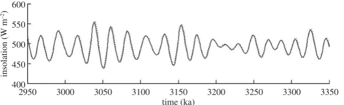
derived from the Laskaret al.[51] (hereafter La93) astronomical solution. Since then, an updated version of the Laskar solution has been produced [49] (hereafter La04). The La04 solution has been improved with respect to La93 by using a direct integration of the gravitational equations for the orbital motion, and by improving the dissipative contributions, in particular, in the evolution of the Earth–Moon system [49]. Before the La04 solution can be used in concert with the LR04 stack to help identify a time slice(s) for reconstruction, we must determine that the solutions provided by La93 or La04 are the same or very similar.Figure 3shows the difference between the two solutions at 65◦

7

rsta.r

oy

alsociet

ypublishing

.or

g

Phil

Tra

ns

R

Soc

A

37

1:

20120515

...

600

550

500

450

insolation (W m

–2)

400

2950 3000 3050 3100 3150 time (ka)

3200 3250 3300 3350

Figure 3.Comparison of insolation at 65◦

N on 21 June between the La93 (dotted curve) versus La04 (solid curve) orbital solutions between 2.95 and 3.35 Ma BP.

the PRISM time slab, the phasing between the two solutions is in strong agreement, as well as the magnitude of the insolation variation. Thus, we are confident in our use of the La04 solution to investigate orbital forcing during the PRISM time slab.

(ii) La04 reconstructions of insolation

Variations in eccentricity, precession and obliquity according to La04 are shown infigure 4b,cfor the period 2.95–3.35 Ma BP. This more than encompasses the PRISM time slab. A notable feature is a low in eccentricity values between 3.20 and 3.30 Ma, with correspondingly low modulations in precession. Across the PRISM time slab, insolation as a global annual mean derived from La04 varies by a maximum of 0.51 W m−2 _{(figure 4f). Largest variations are apparent younger than} 3.2 Ma, with values that are generally closest to modern occurring prior to 3.2 Ma. We have also calculated the difference from present-day insolation at the TOA at each 1000 year time step between 2.95 and 3.35 Ma. This allows us to take into consideration how incoming insolation varies as a function of latitude and month in comparison with present day.

(iii) Statistical evaluation of La04 results

Our objective is to identify times within the PRISM time slab where the TOA insolation distribution is most similar to that of present day. In order to differentiate between the 400 insolation patterns produced, we evaluate the spatial similarity between the past and the present. The match between the spatial patterns has been evaluated in terms of correlation (r), root mean square (r.m.s.) difference and the ratio of the variances (standard deviation, s.d.). A perfect solution under this definition would have no error as computed by the r.m.s., would perfectly correlate with the present (r=_{1), and would have the same standard deviation.}

We consider only solutions within the first 10 discrete minima in root mean square error (r.m.s.e.) as potential candidates for the first Pliocene time slice. This equates to an r.m.s.e. of less than 5 W m−2_{. R.m.s. offers the clearest distinction between the 400 potential solutions, as} s.d. does not vary significantly among the ensemble. Each of the 10 defined minima in r.m.s.e. can include a number of individual orbital solutions that have very similar skill in matching the modern insolation distribution and are closely associated in time (table 1). Best-fitting orbital solutions from each discrete minima in r.m.s.e. are highlighted as vertical lines infigure 4.

8

rsta.r

oy

alsociet

ypublishing

.or

g

Phil

Tra

ns

R

Soc

A

37

1:

20120515

...

3.0

(a)

(b)

(c)

(d)

(e)

(f)

24.0

23.5

23.0

22.5

eccentricity precession

0.05

–0.05

30

20

10

0

1.00

0.99

0.98

342.6

342.0 341.8 342.2 342.4 0 3.5

LR04

d

18O

obliquity

r.m.s.

correlation

insolation (W m –2)

2950 3000 3050 3100 3150 3200 3250 3300 3350

time (ka)

Figure 4.(a) The Lisiecki & Raymo [38] benthic oxygen isotope stack; (b) obliquity, with dashed horizontal line showing the present-day value; (c) precession and eccentricity as derived from the astronomical solution of Laskaret al.[49] (La04), with horizontal dotted black and solid red lines showing present-day values for eccentricity and precession; (d) the calculated r.m.s.e. (W m−2_{) and (e) correlation coeicient (0–1) for orbital solution considered for the Pliocene time slice; and (f) the variation in}

global mean TOA insolation according to La04, with the dotted horizontal green line denoting the modern value of global mean insolation. The vertical solid lines through each panel represent the best-itting solutions considered in the study (black) and the discrete minimum in r.m.s.e. identiied as the Pliocene time slice (solid red).

(c) Characteristics of the irst Pliocene time slice

The chosen time slice sits in the normal polarity of the Gauss Chron between the Kaena (above)

and Mammoth (below) reversals (figure 2). The peak deviation in benthicδ18_{O is centred on}

marine isotope stage (MIS) KM5c (or KM5.3). The 0.21–0.23_{deviation in}δ18_{O could reflect a}

21–23 m sea-level rise above modern (assuming 0.1_{equates to approx. 10 m of sea-level rise),}

providing that the signal is purely a function of ice volume rather than any change in deep-ocean temperatures. Assuming the near-total loss of the West Antarctic and Greenland ice sheets (a reasonable initial premise given proxy data and model outputs [18,20–22]), volume reduction from the East Antarctic ice sheet is a moderate 6 or 7 m of ice volume equivalent. This general interpretation of sea level from the LR04 stack is supported by a recent synthesis of sea-level records between 2.9 and 3.3 Ma BP by Milleret al.[23]. At approximately 3.205 Ma BP, the Miller

et al.[23] synthesis indicates a maximum sea-level rise of 25±_{10 m (derived from Mg/Ca ratios}

of deep marine ostracods [52]). A mean of multiple sea-level records for approximately the same time indicate a peak sea-level rise of approximately 22±_{10 m.}

9

rsta.roy

alsocietypublishing

.or

g

Phil

Tra

nsR

Soc

A3

71:

20120515

.. .. .. ..

deviation (s.d.) from modern for each time point and an assessment of how well each discrete r.m.s. minimum matches the established criteria for the selection of the Pliocene time slice (see §2a). The discrete r.m.s. minimum highlighted initalicsis encompassed by the selected interval time slice reconstruction.

r.m.s.

minima best-itting

(r.m.s. age range time point INS r.m.s. CC s.d.

<5 W m−2_{) (ka) (ka) (W m}−2_{) (W m}−2_{) (0–1) (W m}−2_{) description}

1 3002–3004 3003 0.0532 4.1162 0.9997 158.4268 not situated at or near a discrete negative peak in LR04 stack

. . . .

2 3118–3121 3119 0.0433 3.4920 0.9998 185.4160 not situated at or near a discrete negative peak in LR04 stack, but just above the base of the Kaena reversal (3116 ka;) in the Gauss Normality Chron (C2An.2n) [3]

. . . .

3 3185–3186 3185 0.0606 4.6702 0.9996 158.3028 situated on a descending (towards positive) limb between two negative peaks

. . . .

4 3204–3207 3205 −0.0218 4.2657 0.9996 158.1467 centred on a broad peak(negative excursion), with Mammoth reversal

(C2An.2r)directly before(3207 ka) [3]

. . . .

5 3219 3219 −_{0.0204 4.9019 0.9995 158.0499 within an isotopically light period, but on the falling limb with values}

becoming less negative

. . . .

6 3236–3240 3238 0.0118 1.4689 1.0000 158.2245 in the transition zone towards a negative peak

. . . .

7 3258–3260 3259 0.0296 2.9629 0.9998 158.1762 not situated at or near a discrete negative peak in LR04 stack

. . . .

8 3276–3280 3278 −0.0070 1.1293 1.0000 158.2666 not situated at or near a discrete negative peak in LR04 stack

. . . .

9 3293–3296 3295 −_{0.0014 1.4502 1.000 158.0723 situated at peak in positive isotopic excursion (M2 event)}

. . . .

10 3114 3314 0.0641 4.7294 0.9996 158.3965 outside of PRISM time slab and on a trend towards more positive isotope values

. . . .

on August 21, 2014

rsta.royalsocietypublishing.org

10

rsta.r

oy

alsociet

ypublishing

.or

g

Phil

Tra

ns

R

Soc

A

37

1:

20120515

...

TOA insolation D_{TOA insolation}

modern 90°N

(a) (b) (c)

600 60

48

36

24

12

0

–12

–24

–36

–48

–60

60

48

36

24

12

0

–12

–24

–36 –48

–60 550

500 450 400 350 300 250 200 150 100 50 0

60°N

30°N

30°S

60°S

90°S

Jul Oct Jan Apr Jul Jul Oct Jan Apr Jul Jul Oct Jan Apr Jul 0

3060 ka 3205 ka

Figure 5.(a) Insolation distribution at the top of the atmosphere (TOA) in W m−2_{for the modern; and the insolation anomaly}

between modern and (b) 3060 ka and (c) 3205 ka (derived from the La04 astronomical solution). The time 3060 ka is a time point during the PRISM time slab that exhibits the largest negative excursion in the benthic oxygen isotope record [38] (igure 4). The time 3205 ka is the time point identiied in this study that satisies the outlined criteria for being chosen as the Pliocene time slice.

Table 2.The orbital parameters of eccentricity, precession and obliquity for modern and the Pliocene time slice (3.205 Ma BP) according to the astronomical solution of Laskaret al.[49].

obliquity

time point eccentricity precession (deg)

modern 0.016702 0.016280 23.4393

. . . .

3205 ka 0.007483 0.006048 23.4736

. . . .

remains near modern before and after the time slice. Therefore, the time slice is centred on an interval with a relatively stable orbit during which the distribution of insolation was close to modern (i.e. r.m.s.e. is low, and the correlation coefficient is high).

Available proxy data for atmospheric CO2(see reference [53] for a summary) places an upper limit of approximately 400 ppmv, with a cluster of four measurements within 100 ka of the time slice using three different proxy techniques (alkenones, boron isotopes and stomatal density) indicating a range between 300 and 380 ppmv. These concentrations are broadly supported by new high-resolution alkenone-proxy CO2measurements presented by Badgeret al. [54].

4. Current state of knowledge and future outlook

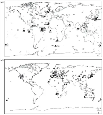
(a) Availability of marine and terrestrial proxy data

Recent advances in deep-sea drilling techniques have made possible the generation of numerous high-resolution orbitally tuned chronologies for Neogene marine sequences. Demand for finer-resolution deep-time palaeoclimate analysis makes this the norm rather than a rarity. The current PRISM SST dataset has 115 sites [17] (figure 6a) focused on a time slab of approximately 240 ka

based on the warm peak averaging technique [35,55]. The next PRISM SST reconstruction,

which is in development (PRISM4), represents more than a two order-of-magnitude increase in resolution with palaeoceanographic reconstruction [56]. Preliminary analysis of available material for reanalysis from the PRISM project suggests that no fewer than 30 globally distributed SST sites may contribute to the first phase of time slice reconstruction for 3.204–3.207 Ma BP (figure 6aand

table 3). These sites range from approximately 50◦

south to approximately 60◦

11

rsta.r

oy

alsociet

ypublishing

.or

g

Phil

Tra

ns

R

Soc

A

37

1:

20120515

...

(a)

(b)

Figure 6.(a) Distribution of PRISM marine sites (open circles) and locations of potential time slice SST data (triangles). The existing PRISM time slab reconstruction (PRISM3D) is conined to a time slab with duration 240 ka, whereas the SST dataset currently in development (PRISM4) represents a signiicant development towards a time slice centred on MIS KM5c (KM5.3). (b) Distribution of PRISM3D terrestrial palaeobotanical sites (illed circles) and locations ofpotentialtime slice vegetation data (triangles).

13 SST records are currently available sampling the high latitudes (IODP sites 1090, 607, 982 and 882), upwelling regions (IODP sites 1082, 847, 847 and 846) and equatorial regions (IODP sites 662, 722, 763, 214 and 806).

Salzmannet al.[8] describe terrestrial proxy data, 202 globally distributed sites, which were synthesized to create a global land-cover reconstruction for the entire Piacenzian Stage.Figure 6b

andtable 4show the distribution of 26 terrestrial localities from the original dataset of 202 sites, which potentially may be able to provide vegetation data to evaluate climate model predictions for the Pliocene time slice. In reality, correlating terrestrial data to any Pliocene time slice is not possible with the same degree of confidence as the marine proxy data. This will require consideration when terrestrial data–model mismatches are highlighted.

12

rsta.r

oy

alsociet

ypublishing

.or

g

Phil

Tra

ns

R

Soc

A

37

1:

20120515

...

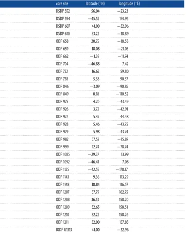
Table 3.Preliminary list of sites included in the existing PRISM time slab SST dataset capable of providing SSTs to support the new time slice reconstruction (igure 6a).

core site latitude (◦

N) longitude (◦

E)

. . . .

DSDP 552 56.04 −23.23

. . . .

DSDP 594 −_{45.52 174.95}

. . . .

DSDP 607 41.00 −_32.96

. . . .

DSDP 610 53.22 −18.89

. . . .

ODP 658 20.75 −_18.58

. . . .

ODP 659 18.08 −_21.03

. . . .

ODP 662 −1.39 −11.74

. . . .

ODP 704 −46.88 7.42

. . . .

ODP 722 16.62 59.80

. . . .

ODP 758 5.38 90.37

. . . .

ODP 846 −3.09 −90.82

. . . .

ODP 849 0.18 −_110.52

. . . .

ODP 925 4.20 −_43.49

. . . .

ODP 926 3.72 −42.91

. . . .

ODP 927 5.47 −_44.48

. . . .

ODP 928 5.46 −_43.75

. . . .

ODP 929 5.98 −43.74

. . . .

ODP 982 57.52 −15.87

. . . .

ODP 999 12.74 −_78.74

. . . .

ODP 1085 −29.37 13.99

. . . .

ODP 1092 −46.41 7.08

. . . .

ODP 1125 −_42.55 −_178.17

. . . .

ODP 1143 9.36 113.29

. . . .

ODP 1148 18.84 116.57

. . . .

ODP 1207 37.79 162.75

. . . .

ODP 1208 36.13 158.20

. . . .

ODP 1209 32.65 158.51

. . . .

ODP 1210 32.22 158.26

. . . .

ODP 1211 32.00 157.85

. . . .

IODP U1313 41.00 −32.96

. . . .

practical sampling resolution in each core. MIS KM2 provides another isotopic marker useful for reference after the time slice itself. We term this interval between MIS M2 and KM2 the

13

rsta.r

oy

alsociet

ypublishing

.or

g

Phil

Tra

ns

R

Soc

A

37

1:

20120515

...

Table 4.Preliminary list of terrestrial sites included in the PRISM time slab dataset [8]potentiallycapable of providing vegetation data to support the new time slice reconstruction (igure 6b).

map ID site latitude (◦

N) longitude (◦

E)

1 ODP 646, Labrador Sea 58.22 −48.20

. . . .

2 ODP 646, Leg 105 58.21 −_48.37

. . . .

3 Great Salt Lake, UT 41.00 −_112.50

. . . .

4 DSDP 467, Leg 63 33.85 −120.76

. . . .

5 ODP 642, Norwegian Sea 67.22 2.94

. . . .

6 La Londe, Normandy 49.31 0.95

. . . .

7 Alpes-Maritimes 43.82 7.19

. . . .

8 DSDP 380, LEG 42B 42.10 29.61

. . . .

9 Rio Maior 39.35 −_8.93

. . . .

10 Andalucia G1 36.38 −4.75

. . . .

11 Tarragona 40.83 1.13

. . . .

12 Bianco/Bovalino 38.25 16.40

. . . .

13 Hula Basin 33.00 35.60

. . . .

14 Nador 35.18 −2.93

. . . .

15 ODP 658, Cape Blanc 20.75 −_18.58

. . . .

16 Hadar 11.29 40.63

. . . .

17 DSDP 231, Leg 24 11.89 48.25

. . . .

18 DSDP 532, Leg 75 −_{21.09 14.46}

. . . .

19 ODP 1082 −_{21.10 11.82}

. . . .

20 Yumen, Jiuxi Basin 39.78 97.53

. . . .

21 Xifeng, Loess Plateau 35.88 107.97

. . . .

22 Himi Area, Toyama 37.15 137.25

. . . .

23 ODP 794A 40.19 138.22

. . . .

24 DSDP 440B/438A 40.00 143.60

. . . .

25 Yallalie, Perth −_{30.43 115.77}

. . . .

26 ODP 1123, Leg 181 −_41.78 −_171.50

. . . .

(b) Enduring uncertainties: challenges and new opportunities

14

rsta.r

oy

alsociet

ypublishing

.or

g

Phil

Tra

ns

R

Soc

A

37

1:

20120515

(a)

(b)

(c)

(d)

(e)

(f)

(g)

(h)

(i)

(j)

(k)

(l)

(m)

(n)

(o)

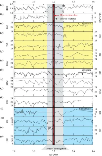
2.7 8 4 0 29 27 27 26 25 24 28 26 24 28 26 24 15 12 9 6 22 20 18 25 3.9 28 26 24 27 25 23 30 28 26 29 27 25 23 28 26 24 21 18 15 12 20 16 12 8

2.8 3.0 3.2

age (Ma) zone of investigation

3.4 3.6 3.3 LR04 662 763 806w 847w 1082 982 1090 607 882 847d 846 214 722 D WT (°C) 3.0 3.2 KM2 M2

zone of tolerance

equatorial

upwelling

high latitudes

Pliocene time slice

3.4 3.6

Figure 7.A compilation of published records of SST that span the late Pliocene and encompass the time slice study proposed here. All SST data are from IODP sites. The red line corresponds to the ideal target identiied by the orbital forcing comparison (igure 5). The dark grey shading highlights a broader time window within which SST estimates could be derived and in all probability still relect conditions during the time slice itself (zone of tolerance). The light grey shading highlights an interval for study to help identify the time slice in marine records, and also to understand climate variability before and after the time slice (zone of investigation). SST records (◦

C) are compared with (a) the benthicδ18_{O stack, LR04 [38] and (b) the deep-water}

15

rsta.r

oy

alsociet

ypublishing

.or

g

Phil

Tra

ns

R

Soc

A

37

1:

20120515

...

annual SAT DJF SAT JJA SAT

–5 –4 –3 –2 –1 0 1 2 3 4 5

3205 minus PRISM3

3195 minus 3205

3215 minus 3205

3060 minus 3205

80' N (a)

(b)

(c)

(d) 40' N

40' S

80' S 0

80' N

40' N

40' S

80' S 0

80' N

40' N

40' S

80' S 0

80' N

40' N

40' S

80' S 0

180 120' W 60' W 0 60' E 120' E 180180 120' W 60' W 0 60' E 120' E 180180 120' W 60' W 0 60' E 120' E 180

Figure 8.Annual mean and seasonal mean (December, January and February, DJF; June, July and August, JJA) Pliocene surface air temperature predictions from HadCM3. (a) Identiied time slice minus a Pliocene experiment with a modern orbital coniguration (PRISM3). Pliocene experiments given orbital conigurations appropriate to (b) 3195 and (c) 3215 ka BP (3195 and 3215 ka minus 3205 ka BP). (d) An experiment for the MIS K1 PlioMAX super interglacial event minus the identiied time slice at 3205 ka BP characterized by a near modern orbital coniguration.

To provide an initial assessment of the degree to which differences in insolation calculated for the 3205 ka BP time slice compared with modern can affect a climate model’s simulation of Pliocene climate, we show the difference in mean annual as well as seasonal average surface air temperatures (SATs) between two Pliocene simulations using the Hadley Centre coupled climate

model version 3 (HadCM3;figure 8). The deviation in SATs as an annual and seasonal mean is

no more than 1◦

C in most ocean and terrestrial regions. The majority of the differences are not statistically significant at a 95% confidence interval (CI).

To provide an initial assessment of how stable climate could have been in response to orbital forcing around the time slice itself, we show results from two further sensitivity studies in which the model has been run with orbital forcing equivalent to 3195 and 3215 ka BP, 10 ka either side of the identified time slice at 3205 ka BP. Compared with mean annual SATs simulated

for the time slice, simulations for 3195 and 3215 ka BP rarely differ by more than 1◦

C. The predicted differences are normally insignificant at a 95% CI. One exception to this is in the North Atlantic, where differences reach 2–3◦

C and are statistically significant (figure 8). The pattern of SAT anomalies is akin to a North Atlantic Oscillation (NAO) dipole, and the results even appear to show the Pacific branch of the Arctic Oscillation (AO). This suggests a few scenarios for the genesis of the changes in the North Atlantic. They may represent a temporal shift of

16

rsta.r

oy

alsociet

ypublishing

.or

g

Phil

Tra

ns

R

Soc

A

37

1:

20120515

...

oscillations. Alternatively, they may represent changes in modes of interannual variability, or be indicative of significant orbital impact on NAO. Providing that these differences are not a model or statistical artefact, the results imply that in the North Atlantic correlation to the time slice would have to be better than 10 ka to keep orbital forcing biases on temperature to less than 3◦C. Seasonally larger changes that are statistically significant are predicted: for example, 3◦

C over Antarctica during the Southern Hemisphere summer and up to 3◦

C over land

in the simulation for 3195 ka in the Northern Hemisphere summer (figure 8). These seasonal

differences will not affect proxy temperature estimates if the proxy itself truly provides an estimate of mean annual temperature. However, they should be considered in data–model comparisons if a proxy technique has the potential to be biased to a temperature reconstruction for a particular season. Therefore, the selection of the time slice and its characteristic stability in orbital forcing immediately before and after creates a time window in which palaeotemperature information can be imperfectly correlated to the time slice itself, but may still be more or less representative of the general conditions that existed during the time slice. We term this azone of tolerance(figure 7).

To place these differences in climate due to orbital variability around the Pliocene time slice in context, we have performed a final experiment with HadCM3 in which an orbital forcing appropriate to 3060 ka was prescribed. The 3060 ka PlioMAX peak (or super interglacial event) is characterized by one of the lightest benthic oxygen isotope excursions evident in the entire PRISM time slab (MIS K1) [66]. The time 3060 ka BP is characterized by the La04 orbital solution as displaying a dramatically different profile of insolation by month and latitude compared with either present day or the identified Pliocene time slice at 3205 ka BP (figure 5). It is also an interval in which the total amount of insolation as a global annual mean differs from present day, or from the 3205 ka BP time slice, by +_{0.5 W m}−2 _{(figure 4). Figure 8 shows the}

model-predicted differences in annual and seasonal mean SAT for 3060 ka BP compared with the Pliocene

time slice at 3205 ka BP. As an annual mean, SAT differences can exceed +₃◦_{C and are almost}

always statistically significant at a 95% CI. This general increase in mean annual temperature is partly caused by the 0.5 W m−2_{enhancement in annual global mean insolation calculated for} 3060 ka BP compared with 3205 ka BP. It is also strongly influenced by much larger changes in seasonal insolation patterns and SATs, which often exceed+₅◦_{C, particularly during the Northern}

Hemisphere summer months (June–August) over the land. If any proxy data included in either the PRISM3D marine or terrestrial environmental reconstructions are actually representative of 3060 ka BP, then it would not be expected to concur with model simulations for the Pliocene set up with a modern, or essentially modern, profile of insolation. This analysis also suggests that 3060 ka BP is inappropriate as a means to assess climate or Earth system sensitivity due to the significant orbital overprint on SATs (figures5and8).

Even with greater certainty in the orbital forcing given to models for the Pliocene, many of the challenges in deriving certain boundary conditions for models remain constant across a time slab or time slice approach. Perhaps the most challenging is the initial state of the ice sheets. The time slice approach also means that the application of a time slab-based vegetation reconstruction as a boundary condition becomes more difficult to justify, implying that future experiments for time slices during the Pliocene will be increasingly dominated by coupled ocean–atmosphere–vegetation models, where vegetation is a predicted rather than a prescribed element.

17

rsta.r

oy

alsociet

ypublishing

.or

g

Phil

Tra

ns

R

Soc

A

37

1:

20120515

...

other techniques to sufficiently explore uncertainty space with climate models, such as a Latin

hypercube approach that has been successfully applied in palaeoclimate research [67], may be

required. The implementation of such a strategy will generate progressively more rigorous data– model comparisons, where an identified signal or residual may highlight a deficiency in climate model predictions for the Pliocene with greater confidence.

Finally, from the point of view of understanding the Pliocene, it is essential to develop a better appreciation of how climate varied through time. We have identified other time slices prior to 3.2 Ma BP that provide potential targets for environmental reconstruction. Of particular interest is the evolution of Pliocene climate and environments from the M2 to KM2 ‘glacial’

events (the zone of investigation identified infigure 7). Until more is understood about how

climate evolved towards and away from the Pliocene time slice, we will not be able fully understand what the time slice represents. Through increasing our understanding of the nature and variability of Pliocene climates, we can understand the Pliocene world more completely, and, at the same time, apply the Pliocene as a test for models used to predict future climate change with increasing certainty.

5. Conclusions

In this study, we outlined the rationale and criteria for the definition of a discrete time slice for environmental reconstruction during the mPWP. The mPWP time slab concept, developed by the US Geological Survey PRISM project, has provided a means to explore and understand climate and environments of a warm phase in Earth history in considerable detail. However, a change in methodology to time slice reconstructions, which have been used so successfully in the Quaternary, is necessary to reduce uncertainties in environmental reconstruction as well as climate/environment modelling. While a range of time slices should be studied that examine different facets of Pliocene climate (e.g. periods with strong orbital forcing or Pliocene ‘glacial’ events), the highest initial priority is to examine a warm period in which orbital forcing was the same as or very similar to present day. This is justifiable given the current requirements to better understand climate and Earth system sensitivity, and to robustly evaluate models used for climate change prediction.

A suitable time slice representative of a warm event or ‘interglacial’ within the existing PRISM time slab has been identified through the calculation and statistical evaluation of orbital forcing using the La04 orbital solution. The time slice is centred on a negative peak (0.21–

0.23_{) in the LR04 benthic oxygen isotope stack at MIS KM5c (KM5.3) at 3.204–3.207 Ma BP.}

Limits of chronology and correlation mean that the time slice may not be resolved in marine records from different ocean basins to a window of only a few thousand years. However,

between 3.215 and 3.195 Ma BP, orbital forcing was similar to present day. Atmospheric CO2

may have peaked at approximately 400 ppmv, with CO2proxies supporting a common range of

between 300 and 380 ppmv. While challenges and uncertainties will remain from a modelling and environmental reconstruction standpoint, the reduced temporal range of a time slice facilitates the construction of more focused sensitivity studies using climate models. Time slices are also short enough to contemplate performing fully transient simulations with a full-complexity intermediate-resolution climate model in the future.

Acknowledgements. The paper forms part of the US Geological Survey Pliocene Research Interpretations and Synoptic Mapping (PRISM) project.

18

rsta.r

oy

alsociet

ypublishing

.or

g

Phil

Tra

ns

R

Soc

A

37

1:

20120515

...

contributions made by the National Centre for Atmospheric Science and the British Geological Survey. D.J.L. acknowledges Research Councils UK for the award of an RCUK fellowship and the Leverhulme Trust for the award of a Phillip Leverhulme Prize.

References

1. Dowsett HJ et al. 2010 The PRISM3D paleoenvironmental reconstruction. Stratigraphy 7_,

123–139.

2. Haywood AMet al. 2010 Pliocene model intercomparison project (PlioMIP): experimental

design and boundary conditions (experiment 1).Geosci. Model Dev.3_{, 227–242. (doi:10.5194/}

gmd-3-227-2010)

3. Gradstein FM, Ogg JG, Smith AG (eds). 2004 A geologic time scale 2004. Cambridge, UK:

Cambridge University Press.

4. Dowsett HJ, Thompson RS, Barron JA, Cronin TM, Fleming RF, Ishman SE, Poore RZ, Willard DA, Holtz TR. 1994 Joint investigations of the middle Pliocene climate. I. PRISM

paleoenvironmental reconstructions. Glob. Planet. Change 9_{, 169–195. (}

doi:10.1016/0921-8181(94)90015-9)

5. Dowsett H, Barron J, Poore R. 1996 Middle Pliocene sea surface temperatures: a global reconstruction.Mar. Micropaleontol.27_{, 13–26. (doi:10.1016/0377-8398(95)00050-X)}

6. Dowsett HJ, Robinson MM, Foley KM. 2009 Pliocene three-dimensional global ocean temperature reconstruction.Clim. Past5_{, 769–783. (doi:10.5194/cp-5-769-2009)}

7. Thompson RS, Fleming RF. 1996 Middle Pliocene vegetation: reconstructions, paleoclimatic inferences, and boundary conditions for climatic modelling.Mar. Micropaleontol.27_{, 27–49.}

(doi:10.1016/0377-8398(95)00051-8)

8. Salzmann U, Haywood AM, Lunt DJ, Valdes PJ, Hill DJ. 2008 A new global biome reconstruction and data–model comparison for the middle Pliocene.Glob. Ecol. Biogeogr.17_,

432–447. (doi:10.1111/j.1466-8238.2008.00381.x)

9. Dowsett HJ, Cronin TM. 1990 High eustatic sea level during the middle Pliocene:

evidence from the southeastern U.S. Atlantic Coastal Plain. Geology 18_{, 435–438.}

(doi:10.1130/0091-7613(1990)018<0435:HESLDT>2.3.CO;2)

10. Sohl LE, Chandler MA, Schmunk RB, Mankoff K, Jonas JA, Foley KM, Dowsett HJ. 2009

PRISM3/GISS topographic reconstruction. U.S. Geol. Surv. Data Series 419. (http://pubs. usgs.gov/ds/419/)

11. Chandler M, Rind D, Thompson R. 1994 Joint investigations of the middle Pliocene

climate. II. GISS GCM Northern Hemisphere results. Glob. Planet. Change 9_{, 197–219.}

(doi:10.1016/0921-8181(94)90016-7)

12. Sloan LC, Crowley TJ, Pollard D. 1996 Modeling of middle Pliocene climate with the NCAR GENESIS general circulation model.Mar. Micropaleontol.27_{, 51–61. (}

doi:10.1016/0377-8398(95)00063-1)

13. Haywood AM, Valdes PJ, Sellwood BW. 2000 Global scale palaeoclimate reconstruction of

the middle Pliocene climate using the UKMO GCM: initial results.Glob. Planet. Change 25_,

239–256. (doi:10.1016/S0921-8181(00)00028-X)

14. Haywood AM, Valdes PJ. 2004 Modelling middle Pliocene warmth: contribution of atmosphere, oceans and cryosphere.Earth Planet. Sci. Lett.218_{, 363–377. (}

doi:10.1016/S0012-821X(03)00685-X)

15. Lunt DJ, Haywood AM, Schmidt GA, Salzmann U, Valdes PJ, Dowsett HJ. 2010 Earth system sensitivity inferred from Pliocene modelling and data. Nat. Geosci.3_{, 60–64. (doi:10.1038/}

ngeo706)

16. Dowsett HJ, Haywood AM, Valdes PJ, Robinson MM, Lunt DJ, Hill DJ, Stoll DK, Foley KM. 2011 Sea surface temperatures of the mid-Piacenzian warm period: a comparison

of PRISM3 and HadCM3. Palaeogeogr. Palaeoclimatol. Palaeoecol. 309_{, 83–91. (doi:10.1016/}

j.palaeo.2011.03.016)

17. Dowsett HJet al.2012 Assessing confidence in Pliocene sea surface temperatures to evaluate predictive models.Nat. Clim. Change2_{, 365–371. (doi:10.1038/nclimate1455)}

18. Lunt DJ, Foster GL, Haywood AM, Stone EJ. 2008 Late Pliocene Greenland glaciation

controlled by a decline in atmospheric CO2 levels. Nature 454, 1102–1106. (doi:10.1038/

19

rsta.r

oy

alsociet

ypublishing

.or

g

Phil

Tra

ns

R

Soc

A

37

1:

20120515

...

19. Hill DJ, Dolan AM, Haywood AM, Hunter SJ, Stoll DK. 2010 Sensitivity of the Greenland ice sheet to Pliocene sea surface temperatures.Stratigraphy7_{, 111–122.}

20. Naish Tet al.2009 Obliquity-paced Pliocene West Antarctic ice sheet oscillations.Nature458_,

322–328. (doi:10.1038/nature07867)

21. Pollard D, DeConto RM. 2009 Modelling West Antarctic ice sheet growth and collapse through the past five million years.Nature458_{, 329–332. (doi:10.1038/nature07809)}

22. Dolan AM, Haywood AM, Hill DJ, Dowsett HJ, Hunter SJ, Lunt DJ, Pickering S. 2011 Sensitivity of Pliocene ice sheets to orbital forcing.Palaeogeogr. Palaeoclimatol. Palaeoecol.309_,

98–110. (doi:10.1016/j.palaeo.2011.03.030)

23. Miller KG et al.2012 High tide of the warm Pliocene: implications of global sea level for

Antarctic deglaciation.Geology40_{, 407–410. (doi:10.1130/G32869.1)}

24. Dekens PS, Ravelo AC, McCarthy MD. 2007 Warm upwelling regions in the Pliocene warm period.Paleoceanography22_{, PA3211. (doi:10.1029/2006PA001394)}

25. Cronin TM, Whatley RC, Wood A, Tsukagoshi A, Ikeya N, Brouwers EM, Briggs WM. 1993 Microfaunal evidence for elevated mid-Pliocene temperatures in the Arctic Ocean.

Paleoceanography8_{, 161–173. (doi:10.1029/93PA00060)}

26. Polyak Let al.2010 History of sea-ice in the Arctic.Quat. Sci. Rev.29_{, 1757–1778. (doi:10.1016/}

j.quascirev.2010.02.010)

27. Moran Ket al.2006 The Cenozoic palaeoenvironment of the Arctic Ocean.Nature441_{, 601–605.}

(doi:10.1038/nature04800)

28. Chan WL, Abe-Ouchi A, Ohgaito R. 2011 Simulating the mid-Pliocene climate with the MIROC general circulation model: experimental design and initial results.Geosci. Model Dev. 4_{, 1035–1049. (doi:10.5194/gmd-4-1035-2011)}

29. Wan S, Tian J, Steinke S, Li A, Li T. 2010 Evolution and variability of the East Asian summer monsoon during the Pliocene: evidence from clay mineral records of the South China Sea.

Palaeogeogr. Palaeoclimatol. Palaeoecol.293_{, 237–247. (doi:10.1016/j.palaeo.2010.05.025)}

30. Salzmann U, Haywood AM, Lunt DJ. 2009 The past is a guide to the future? Comparing middle Pliocene vegetation with predicted biome distributions for the twenty-first century.

Phil. Trans. R. Soc. A367_{, 189–204. (doi:10.1098/rsta.2008.0200)}

31. Hansen Jet al.2008 Target atmospheric CO2: where should humanity aim?Open Atmos. Sci. J.

2_{, 217–231. (doi:10.2174/1874282300802010217)}

32. Charney Jet al.1979Carbon dioxide and climate: a scientific assessment. Washington, DC: National Academy of Sciences.

33. Meinshausen M, Meinshausen N, Hare W, Raper SCB, Frieler K, Knutti R, Frame DJ, Allen

MR. 2009 Greenhouse-gas emission targets for limiting global warming to 2◦

C.Nature458_,

1158–1162. (doi:10.1038/nature08017)

34. Haywood AM, Ridgwell A, Lunt DJ, Hill DJ, Pound MJ, Dowsett HJ, Dolan AM, Francis JE, Williams M. 2011 Are there pre-Quaternary geological analogues for a future greenhouse

gas-induced global warming? Phil. Trans. R. Soc. A 369_{, 933–956. (doi:10.1098/rsta.2010.}

0317)

35. Dowsett HJ, Poore RZ. 1991 Pliocene sea surface temperatures of the North Atlantic Ocean at 3.0 Ma.Quat. Sci. Rev.10_{, 189–204. (doi:10.1016/0277-3791(91)90018-P)}

36. Leroy S, Dupont L. 1994 Development of vegetation and continental aridity in northwestern Africa during the late Pliocene: the pollen record of ODP site 658.Palaeogeogr. Palaeoclimatol. Palaeoecol.109_{, 295–316. (doi:10.1016/0031-0182(94)90181-3)}

37. Haywood AM, Valdes PJ, Sellwood BW. 2002 Magnitude of climate variability during middle Pliocene warmth: a palaeoclimate modelling study.Palaeogeogr. Palaeoclimatol. Palaeoecol.188_,

1–24. (doi:10.1016/S0031-0182(02)00506-0)

38. Lisiecki LE, Raymo ME. 2005 A Pliocene–Pleistocene stack of 57 globally distributed benthic δ18_{O records.Paleoceanography}20_{, PA1003. (doi:10.1029/2004PA001071)}

39. Willeit M, Ganopolski A, Feulner G. 2013 On the effect of orbital forcing on mid-Pliocene climate, vegetation and ice sheets.Clim. Past9_{, 1749–1759. (doi:10.5194/cp-9-1749-2013)}

40. Moucha R, Forte AM, Rowley DB, Mitrovica JX, Simmons NA, Grand SP. 2009 Deep mantle forces and the uplift of the Colorado plateau.Geophys. Res. Lett.36_{, L19310. (doi:10.1029/}

2009GL039778)

41. Sarnthein M. 2013 History of Quaternary glaciations. Transition from late Neogene to early

Quaternary environments. InEncyclopedia of Quaternary science, 2nd edn (eds SA Elias, CJ

20

rsta.r

oy

alsociet

ypublishing

.or

g

Phil

Tra

ns

R

Soc

A

37

1:

20120515

...

42. Bartoli G, Sarnthein M, Weinelt M, Erlenkeuser H, Garbe-Schonberg D, Lea DW. 2005 Final closure of Panama and the onset of northern hemisphere glaciations.Earth Planet. Sci. Lett. 237_{, 33–44. (doi:10.1016/j.epsl.2005.06.020)}

43. Des Marais DL, Juenger TE. 2010 Pleiotropy, plasticity, and the evolution of plant abiotic stress tolerance.Ann. NY Acad. Sci.1206_{, 56–79. (doi:10.1111/j.1749-6632.2010.05703.x)}

44. Murray JW. 2001 The niche of benthic foraminifera, critical thresholds and proxies. Mar.

Micropaleontol.41_{, 1–7. (doi:10.1016/S0377-8398(00)00057-8)}

45. Dowsett HJ, Barron JA, Poore RZ, Thompson RS, Cronin TM, Ishman SE, Willard DA. 1999

Middle Pliocene paleoenvironmental reconstruction: PRISM2. USGS Open File Report 99-535. (http://pubs.usgs.gov/openfile/of99-535)

46. IPCC. 2007Climate change 2007: the physical science basis. Contribution of Working Group I to the Fourth Assessment Report of the Intergovernmental Panel on Climate Change(eds S Solomon, D Qin, M Manning, Z Chen, M Marquis, KB Averyt, M Tignor, HL Miller). Cambridge, UK: Cambridge University Press.

47. Otto-Bliesner B, Marshall SJ, Overpeck JT, Miller GH, Hu A, CAPE Last Interglacial project members. 2006 Simulating Arctic climate warmth and ice field retreat in the Last Interglaciation.Science311_{, 1751–1753. (doi:10.1126/science.1120808)}

48. Lunt DJ, Haywood AM, Schmidt GA, Salzmann U, Valdes PJ, Dowsett DJ, Loptson CA. 2012 On the causes of mid-Pliocene warmth and polar amplification.Earth Planet. Sci. Lett.321–322_,

128–138. (doi:10.1016/j.epsl.2011.12.042)

49. Laskar J, Robutel P, Joutel F, Gastineau M, Correia ACM, Levrard B. 2004 A long term numerical solution for the insolation quantities of the Earth.Astron. Astrophys.428_{, 261–285.}

(doi:10.1051/0004-6361:20041335)

50. Berger A, Loutre MF. 1992 Astronomical solutions for paleoclimate studies over the last 3 million years.Earth Planet. Sci. Lett.111_{, 369–382. (doi:10.1016/0012-821X(92)90190-7)}

51. Laskar J, Joutel F, Boudin F. 1993 Orbital, precessional and insolation quantities for the Earth from−_{20 Myr to}+_{10 Myr.Astron. Astrophys.}270_{, 522–533. (http://adsabs.harvard.edu/}

full/1993A&A...270..522L)

52. Dwyer GS, Chandler MA. 2009 Mid-Pliocene sea level and continental ice volume based on

coupled benthic Mg/Ca palaeotemperatures and oxygen isotopes.Phil. Trans. R. Soc. A367_,

157–168. (doi:10.1098/rsta.2008.0222)

53. Bartoli G, Hönisch B, Zeebe RE. 2011 Atmospheric CO2 decline during the Pliocene

intensification of Northern Hemisphere glaciations. Paleoceanography 26_{, PA4213.}

(doi:10.1029/2010PA002055)

54. Badger MPS, Schmidt DN, Mackensen A, Pancost RD. 2013 High-resolution alkenone palaeobarometry indicates relatively stablepCO2during the Pliocene (3.3–2.8 Ma).Phil. Trans.

R. Soc. A371_{, 20130094. (doi:10.1098/rsta.2013.0094)}

55. Dowsett HJ, Robinson MM. 2006 Stratigraphic framework for Pliocene paleoclimate reconstruction: the correlation conundrum.Stratigraphy3_{, 53–64.}

56. Dowsett HJ, Robinson MM, Stoll DK, Foley KM, Johnson ALA, Williams M, Riesselman CR. 2013 The PRISM (Pliocene palaeoclimate) reconstruction: time for a paradigm shift.Phil. Trans. R. Soc. A371_{, 20120524. (doi:10.1098/rsta.2012.0524)}

57. Sosdian S, Rosenthal Y. 2009 Deep-sea temperature and ice volume changes across the Pliocene–Pleistocene climate transitions. Science 325_{, 306–310. (doi:10.1126/science.}

1169938)

58. Herbert TD, Peterson LC, Lawrence KT, Liu Z. 2010 Tropical ocean temperatures over the past 3.5 million years.Science328_{, 1530–1534. (doi:10.1126/science.1185435)}

59. Karas C, Nürnberg D, Tiedemann R, Garbe-Schönberg D. 2011 Pliocene Indonesian throughflow and Leeuwin current dynamics: implications for Indian Ocean polar heat flux.

Paleoceanography26_{, PA2217. (doi:10.1029/2010PA001949)}

60. Karas C, Nurnberg D, Gupta AK, Tiedemann R, Mohan K, Bickert T. 2009 Mid-Pliocene

climate change amplified by a switch in Indonesian subsurface throughflow.Nat. Geosci.2_,

434–438. (doi:10.1038/ngeo520)

61. Wara MW, Ravelo AC, Delaney ML. 2005 Permanent El Niño-like conditions during the Pliocene warm period.Science309_{, 758–761. (doi:10.1126/science.1112596)}

62. Etourneau J, Martinez P, Blanz T, Schneider R. 2009 Pliocene–Pleistocene variability of upwelling activity, productivity, and nutrient cycling in the Benguela region.Geology 37_,

21

rsta.r

oy

alsociet

ypublishing

.or

g

Phil

Tra

ns

R

Soc

A

37

1:

20120515

...

63. Martinez-Garcia A, Rosell-Melé A, McClymont EL, Gersonde R, Haug GH. 2010 Subpolar link to the emergence of the modern equatorial Pacific cold tongue.Science328_{, 1550–1553.}

(doi:10.1126/science.1184480)

64. Lawrence KT, Herbert TD, Brown CM, Raymo ME, Haywood AM. 2009 High-amplitude variations in North Atlantic sea surface temperature during the early Pliocene warm period.

Paleoceanography24_{, PA2218. (doi:10.1029/2008PA001669)}

65. Lawrence KT, Sosdian S, White HE, Rosenthal Y. 2011 North Atlantic climate evolution

through the Plio–Pleistocene climate transitions. Earth Planet. Sci. Lett. 300_{, 329–342.}

(doi:10.1016/j.epsl.2010.10.013)

66. Raymo ME, Mitrovica JX, O’Leary MJ, DeConto RM, Hearty PJ. 2011 Departures from eustasy in Pliocene sea-level records.Nat. Geosci.4_{, 328–332. (doi:10.1038/ngeo1118)}