The effect of variability on the outcome of likelihood ratios

(1)

The effect of variability on the

outcome of likelihood ratios

Vincent Stephen Hughes

September 2011

Supervisor: Prof Paul Foulkes

Submitted in partial fulfilment of the degree of MSc at the Department of

Language and Linguistics, University of York

(2)

ABSTRACT

The likelihood ratio (LR) is the “logically and legally correct” (Rose and Morrison 2009:143) framework for the estimation of strength-‐of-‐evidence under two competing hypotheses. In forensic voice comparison these considerations are reduced to the similarity and typicality of features across a pair of suspect and offender samples. However, typicality can only be judged against patterns in the relevant population (Aitken and Taroni 2004:206). In calculating numerical LRs typicality is assessed relative to a sub-‐section of that population.

This study considers issues of variability relating to the delimitation of reference data with regard to the number of speakers and number of tokens per speaker. Using polynomial estimations of F1 and F2 trajectories from spontaneous GOOSE (Wells 1982), LR comparisons were performed against a reference set of up to 120 speakers and up to 13 tokens per speaker. Results suggest that mean same-‐speaker LRs are robust to such variation until the reference data is limited to small numbers of speakers and tokens. However, variance and severity of error may be continually reduced with the inclusion of more data.

The definition of the relevant population with regard to regional variety is also assessed. Results for LRs are presented across four sets of test data where only one set matches the reference population for accent. In the absence of differences in levels of within-‐speaker variation, the magnitude of same-‐speaker LRs and severity of error are shown to be considerably higher for the ‘mismatch’ test sets. However, results indicate that the removal of regionally-‐defining acoustic information may reduce the effect of accent divergence between the evidential and reference data. This has positive implications for the application of the numerical LR approach.

(3)

LIST OF TABLES

Table 1 – Phonological categorisation of GOOSE tokens and the maximum number of tokens in such contexts shared by all speakers in each of the test sets………

Table 2 – Mean within-‐ and between-‐speaker variation for each of the test sets………..

Table 3 – Percentage of tokens in test and reference data in each of the four phonological contexts coded for………..

Table 4 – Number of speakers in the reference set grouped according to the number of tokens per speaker………

Table 5 – Verbal expressions of raw and log10 LRs according to Champod and Evett’s verbal scale (2000:240)………

Table 6 – Mean within-‐speaker variation (Hz) according to regionally-‐defined test set………

Table 7 – Mean log10 LRs for same-‐speaker pairs from each of the test sets for quadratic and cubic systems………

Table 8 – Percentage of different-‐speakers pairs in the Manchester and Newcastle test sets with LR output which supported the same-‐speaker hypothesis (Hp)……….…

PAGE

(6)

LIST OF FIGURES

Figure 1 – TextGrid of the word ‘moved’ with GOOSE produced by speaker 1 in the Manchester test set………

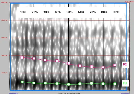
Figure 2 – Spectrogram of GOOSE showing the location of markers at +10% steps at which F1 and F2 measurements were taken………

Figure 3 – F1~F2 plots of mean GOOSE trajectories based on raw acoustic data for all tokens grouped according to regional variety……….

Figure 4 – Mean F1 and F2 formant contours of GOOSE for the eight speakers in each of the regionally defined test data sets together with mean contours for the 120 speakers functioning as the reference set………..

Figure 5 – MDS plot of Euclidean distance between each of the speakers in the test sets and the reference data……….

Figure 6 – Scattergram of the raw F2 contour for GOOSE (‘doing’) relative to the fitted quadratic polynomial curve and the residuals………..

Figure 7 – Scattergram of the raw F1 contour for GOOSE (‘doing’) relative to quadratic and cubic estimations of contour shape……….

Figure 8 – Diagrammatical representation of the MKVD formula modelling of within-‐ and between-‐speaker variation based on +50% measurement of F2 from the current data set with the first and second speakers from the York test data functioning as mock suspect and offender………

Figure 9 – Mean and SD of log10 LRs based on quadratic polynomials for same-‐ and different-‐speaker pairs according to the number of speakers in the reference data………

PAGE

(7)

Figure 10 – Scattergram of standard deviation of log10 LRs for SS and DS pairs relative to the size of the reference population (quadratic polynomials)………..

Figure 11 – Contour of log-‐LR cost plotted against the number of speakers in the reference data set (quadratic polynomials)………..

Figure 12 – Scattergram of log-‐LR cost plotted against between 40 and 120 reference speakers (quadratic polynomials)………

Figure 13 – Mean and SD of log10 LRs based on cubic polynomials for same-‐ and different-‐speaker pairs according to the number of speakers in the reference data………

Figure 14 – Contour of log-‐LR cost plotted against the number of speakers in the reference data set (cubic polynomials)………

Figure 15 – Mean and SD of log10 LRs based on quadratic polynomials for same-‐ and different-‐speaker pairs according to the number of tokens per speaker in the reference data………..

Figure 16 – Scattergram of log-‐LR cost according to the number of tokens per speaker in the reference data (quadratic polynomials).………...

Figure 17 – Mean and SD of log10 LRs based on cubic polynomials for same-‐ and different-‐speaker pairs according to the number of tokens per speaker in the reference data………..

Figure 18 – Scattergram of log-‐LR cost according to the number of tokens per speaker in the reference data (cubic polynomials)………...

Figure 19 – Tippett plot of same-‐speaker comparisons based on quadratic polynomials of F1 and F2 for each of the test sets………...

(8)

Figure 20 – Tippett plot of same-‐speaker comparisons based on cubic polynomials of F1 and F2 for each of the test sets………..

Figure 21 – Scattergram of within-‐speaker variability (Hz) plotted against log10 LRs based on quadratic polynomials for each of the 32 same-‐speaker LR comparisons performed……….

Figure 22 – Scattergram of normalised Euclidean distance from the reference data of each individual speaker in each of the test sets plotted against the log10 LR outcome of the SS comparison based on quadratic polynomials of F1-‐F2 for that individual………

Figure 23 – Tippett plot of different-‐speaker comparisons based on quadratic polynomials of F1 and F2 for each of the test sets………..

Figure 24 – Tippett plot of different-‐speaker comparisons based on cubic polynomials of F1 and F2 for each of the test sets………

Figure 25 – Normalised Euclidean distance between mock different-‐speaker suspect and offender samples plotted against the log10 LR output based on quadratic polynomials of F1-‐F2 for that DS comparison for all speakers in each of the four test sets………

Figure 26 – Combined normalised Euclidean distance of the different speakers acting as suspect and offender plotted against log10 LRs for those DS pairs calculated on the basis of quadratic polynomials……….

Figure 27 – Tippett plot of same-‐speaker comparisons based on quadratic polynomials of F2 for each of the test sets………..……….

Figure 28 – Tippett plot of same-‐speaker comparisons based on cubic polynomials of F2 for each of the test sets………

(9)

Figure 29 – Scattergram of normalised Euclidean distance from the reference data based on quadratic polynomials of F2 for each individual speaker in each of the test sets plotted against the log10 LR outcome of the SS comparison for that individual………

Figure 30 – Tippett plot of different-‐speaker comparisons based on quadratic polynomials of F2 for each of the test sets………

Figure 31 – Tippett plot of same-‐speaker comparisons based on cubic polynomials of F2 for each of the test sets………

Figure 32 – Log-‐LR cost for each of the test sets under each of the experimental conditions (polynomials-‐formants)……….

Figure 33 – MDS plot of the Euclidean distances between the eight Newcastle test speakers, their combined means and the ONZE reference data, with the positing of speaker3 marked relative to the two reference data points….………..

Figure 34 – Linear trendline for the correlation between normalised Euclidean distance from the ONZE reference data and LR output based on quadratic polynomials of F1-‐F2……….

Figure 35 – Calculation used to estimate the LR output for the SS comparison for speaker3 relative to a set of reference data positioned within the speaker space at the mean for the Newcastle test data.……….

Figure 36 – MDS plot of the Euclidean distances between the eight Newcastle test speakers, their combined means and the ONZE reference data, with the positing of speaker1 marked relative to the two reference data points….………..

(10)

ACKNOWLEDGEMENTS

I wish to thank my supervisor Paul Foulkes for all of his encouragement, support and guidance not only during the ‘dissertation months’, but throughout this year of ups and downs. I am also indebted to him and Dom Watt for initially sparking my interest in forensic phonetics in the final year of my undergraduate degree. A huge debt of gratitude is also owed to Ashley Brereton (Dept. of Maths, University of Liverpool). Ash’s willingness to explain mathematical concepts, answer my questions and essentially teach me how to use MatLab goes above and beyond the level of friendship and without his help this dissertation would literally have been impossible. Special thanks go to Phil Harrison for writing the MatLab LR loop function. I can’t even imagine how I would have gone about performing the 273,408 LR calculations in this study without it! It is also necessary to thank Jen Hay and others involved in ONZE for allowing me to use their 96,372 formant measurements. The prospect of extracting this much data by hand was a particularly daunting one. Similarly, thanks to Bill Haddican for providing the Manchester, York and Newcastle data, and to Hazel Richards for putting up with my continual requests for more sound files. For making me look at my results in a different light I thank Rich Rhodes, and although we only met for the first time relatively recently, I am also grateful to Frantz Clermont for his encouragement and inspiration.

On a personal level, the unwavering love and support (both emotional and financial) of my mum and dad has been invaluable and for that I am truly grateful. Thanks also go to my brother Phil. His words of support have perked me up when I’ve been down and I hope that I can be there for him in the same way that he has been there for me. Finally, I wish to thank Fiona for putting up with me and looking after me when times have been tough. Her patience and love have been instrumental not only in the completion of this dissertation, but throughout this year.

(11)

1.0 INTRODUCTION

In the UK voice comparison (FVC) accounts for the vast proportion of casework undertaken by forensic speech scientists (c.70%, French p.c.). Experts are typically presented with two samples (one incriminating sample containing the voice of the offender, the other containing the voice of the suspect) and asked to compare the speech patterns to assess the possibility that the same-‐speaker is present in both.

However, the paradigm shift (Saks and Koehler 2005) across forensic disciplines reflects a move towards the evaluation of such evidence within a framework which is more “scientific” (Morrison 2009a:1). The shift reflects the Court of Appeal’s concern over “the logically correct evaluation and presentation” (Morrison 2009a:1) of expert evidence in R-‐v-‐Doheny and Adams [1996]. The court ruled that DNA evidence presented as posterior probability, i.e. an assessment of the hypotheses given the evidence p(H|E), committed the prosecutor’s fallacy (Thompson and Schumann 1987) and gave undue weight to the expert’s testimony.

With DNA “setting the standard” (Baldwin 2005:55) in forensic science, the Doheny Court’s assertion that “the scientist should not be asked his opinion on the likelihood that it was the Defendant who left the crime stain” (Rose 2007a) emphasises the validity of considering the probability of the evidence rather than the hypotheses. In line with the Court’s judgement, the Bayesian framework, and specifically the likelihood ratio (LR), are now widely accepted as the “logically and legally correct” (Rose and Morrison 2009:143) approach for the estimation of strength-‐of-‐evidence. Despite the Court of Appeal ruling in R-‐v-‐T [2010], Bayes’ theorem forms “the model for a scientifically defensible approach in forensic identification science” (Gonzalez-‐Rodriguez et al 2007:2104) towards which the current shift is moving.

The Bayesian approach provides a framework for the assessment of evidence across a criminal trial and its facility for the incorporation of “multiple piece(s) of evidence” makes it “a very attractive measure for (FVC)” (Kinoshita 2002:300). The odds form of Bayes’ theorem is:

(12)

!

(

!

)

!

(

!

)

!

)

!

! )

!

!)

!

)

Prior Odds Likelihood Ratio Posterior Odds

adapted from Rose (2004:3)

Where

The prior odds reflect the trier-‐of-‐fact’s assessment of the probability of the hypotheses before the introduction of evidence (see Cohen 1982; Redmayne 1998). The prior odds are modified by planks of evidence expressed within a LR framework to establish posterior odds. The posterior odds are concerned with what Lynch and McNally refer to as the “ultimate issue” (2003:96) of innocence or guilt: an assessment of the probability of the hypotheses given the weight of evidence.

Central to Bayes’ theorem is the LR: an estimation of strength-‐of-‐evidence based on its probability of occurrence given Hp divided by the probability of its occurrence given Hd. In FVC, the numerator is equated to the similarity of samples, while the denominator is concerned with their typicality in the

relevant population (Aitken and Taroni 2004:206). Numerical LRs are calculated using acoustic data, where suspect and offender samples are compared against a sampled sub-‐section of the relevant

population. The outcome is a value centred on one, such that LRs of >1 offer support for Hp whilst LRs of <1 offer support for Hd (Rose 2004:4). The magnitude of the LR determines how much more likely the evidence would be given Hx than Hy (Evett et al 2000). A LR of five is interpreted as: ‘the evidence is five times more likely assuming the hypothesis that the same-‐speaker was involved than assuming the hypothesis that different-‐speakers were involved’.

p

p p

d

x

=

d

p = probability

E = evidence | = ‘given’

Hp = prosecution hypothesis (i.e. same-‐speaker)

Hd = defence hypothesis (i.e. different-‐speaker)

(13)

Robertson and Vignaux maintain that “expert evidence should be restricted to the (LR) given by the test or observation of its components” (1995:21). Similarly, Rose describes the role of Bayes’ Theorem in FVC as “non-‐negotiable” (2004:3). Logical and legal arguments for these claims are numerous.

The distinction between assessing the hypotheses and the evidence ensures that the roles of trier-‐ of-‐fact and expert are separated. In restricting the expert to the LR, the ultimate issue remains the preserve of judge and jury. This also prevents the expert from expressing “inappropriate” p(H|E) conclusions based on “information and assumptions from sources other than an objective scientific evaluation of the known and questioned samples” (Morrison 2009a:4). Moreover, it is not only inappropriate but logically impossible for the expert to provide posterior probability. This is because

p(H|E) is dependent on prior odds, which are determined by the trier-‐of-‐fact and therefore inaccessible. Finally, the LR conforms with the US Supreme Court ruling in Daubert [1993] which requires that theories and techniques have been tested and “actual or potential error rates (…) considered” (Rose 2002:121).

However, the LR approach itself does not ensure a reliable estimation of strength-‐of-‐evidence. Numerical LRs are necessarily affected by the input data, such that the removal of an individual from the reference population will vary the outcome. However, very little is known about the robustness of LRs to systematic variability in the reference population and to truly satisfy Daubert, it is essential that error, and LR performance more generally, are assessed under such conditions. Therefore, this study presents an investigation into the issue of variability in the definition and delimitation of the reference population with a focus on population size and accent mismatch.

(14)

2.0 BACKGROUND

2.1 Expression of conclusions in forensic speech science (FSS)

Gold (2011) surveyed 36 forensic speech scientists to investigate how experts frame conclusions in FVC casework. Results reveal a lack of consensus. The highest proportion of experts (39%) currently use a classical probability framework of the kind described in Baldwin and French (1990:10). However, there has been an increasing impetus for FSS to move away from such p(H|E) statements. Initial concerns over classical probability scales were raised in Broeders (1999) and subsequently Champod and Evett (2000) and Champod and Meuwly (2000) argued for the assessment of FVC evidence within a LR framework. In countries where probability scales are in operation there is also growing support for the Bayesian approach (Jessen 2011).

However, contrary to the cross-‐disciplinary paradigm shift, just four experts in Gold (2011) have adopted the numerical LR framework. This reflects concerns over the practical implementation of numerical LRs (Nolan 2001). French and Harrison claim that a quantitative approach is primarily precluded by “the lack of demographic data” (2007:142). This is emphasised by Rose as “one of the main factors that make the accurate estimation of LRs problematic” (2004:4). As a solution, Rose (2007a) proposes that experts collect reference data themselves.

To ensure reliable strength-‐of-‐evidence from such data two issues must be addressed. Firstly, the relevant population needs to be defined and secondly, the sub-‐section of the population must be delimited. However, the task of ensuring that reference data is representative, relevant and reliable is not straightforward. Indeed, Morrison claims that “the only principled objections (to LRs) (…) (are) related to defining the relevant population to sample in order to calculate (…) typicality” (2009a:13).

2.2 The ‘defence hypothesis’

(15)

impossible to determine the probability of the evidence with a vague and ill-‐defined hypothesis” (1995:31). In many jurisdictions the defence will offer simply a ‘different-‐speaker’ hypothesis or no alternative at all. Rose claims that in such cases Hd may be assumed to be “another same-‐sex speaker of the language” (2004:4).

Coleman and Walls define the relevant population as “those persons who could have been involved (ignoring other priors)” (1974:276). Smith and Charrow propose a modification, claiming that typicality should be assessed against “the smallest population known to possess the culprit as a member” (1975:556). Lenth (1986) justifies the need for a more specific hypothesis than ‘it was a different speaker’, arguing that the LR model assumes that “the alleged source of the evidence is a random selection from those persons having the required characteristics” (in Aitken 1991:58). Therefore, only when “there is no evidence to separate the perpetrator from the (…) population” or “results can be regarded as independent of variations in sub-‐groups” (Robertson and Vignaux 1995:36) should a ‘general’ population be used. Given the inferences which may be made about an individual on the basis of his speech patterns, in most cases the relevant population may be defined more narrowly than the default assumption in Rose (2004). Such inferences relate to regional background, age and class amongst others.

However, in reality it is not possible to define the reference population on the basis of all social groups to which the perpetrator belongs. In other areas of forensic science this issue may be resolved by logical relevance (Kaye 2004). In DNA casework Hd is determined in part by ethnicity since the frequency of certain strands is variable according to ethnic groupings. As offender ethnicity cannot be inferred from DNA alone, a multiple-‐Hd approach is adopted in which the jury is presented with LRs according to the ethnic grouping of the reference population (Kaye 2008). Since ethnicity affects the magnitude of the LR it is considered logically relevant.

2.3 LR-‐based studies in FSS

(16)

strength-‐of-‐evidence, despite the small number of speakers. Rose, Osanai and Kinoshita (2003) investigated LR performance based on a multivariate analysis of cepstral coefficients and formants from a nasal, voiceless fricative and vowel. Again intrinsic testing was performed based on 60 male Japanese speakers from 11 prefectures. The test data was also uncontrolled for age.

Alderman (2004) assessed the viability of the Bernard data (Bernard 1967, 1970) as a reference distribution for FVC. By focussing on the role of the reference data, the study represents the first step towards tackling this “deficiency in the (LR) method” (Rose 2002:320). Whilst the age of test speakers is restricted, Alderman claims that three accent groupings based on ‘broadness’ in Australian English are adequate “for a number of difference variations of (Hd) based on accent” (2004:511). However, the viability of the Bernard data is determined on the strength-‐of-‐evidence and LRtest (the ratio of SS pairs achieving LRs of >1 to DS pairs achieving LRs of <1) achieved for individual phonemes, rather than the comparative performance of accent groupings.

Extrinsic testing, involving an independent reference set of 166 speakers was performed by Rose et al (2006) based on formant trajectories of /aɪ/. Sound change in the form of a lowering of F2 at the onset and increase in F1 at the offset during the 30 years which separates the reference and test recordings is claimed to be “important” (2006:330). However, no predictions are made as to the expected effects of such change and no reference is made to this when discussing the results.

Morrison’s (2008) study of /aɪ/ explicitly acknowledges potential sources of variation which may affect LR output. Morrison highlights the age range of 19 to 64 years, small number of speakers (intrinsic testing using 27 speakers) and the presence of “some dialect variation” (2008:251) as potential shortcomings of the method employed. Zhang et al’s (2011) study of Chinese /i au/

displays a more active consideration of the issues in Morrison (2008). Despite the small reference population (20 speakers), there is greater control over regional background and age. Therefore, the speakers in Zhang et al are a more homogeneous set than those previously investigated in numerical LR studies. Finally, regional variety is also raised by Rose as a factor which makes a “minimal contribution to the good results” (2011:1721) based on formants and cepstral coefficients from two tokens of five vowel phonemes in Japanese.

(17)

for greater controls over the definition of the reference population. Loakes claims that if the sample is not representative, “the resulting LR will in turn be misrepresentative” (2006:197) and suggests that along with “speaker sex and accent (…) tighter constraints on social variables might also need to be applied to population selection” (2006:198).

Systematic research into the effect of variability in the reference data is offered by Ishihara and Kinoshita (2008) and Hawkins and Clermont (2009). Both found that the number of reference speakers can dramatically affect LR output, especially when this number is limited. Further, Hawkins and Clermont (2009) show a broadening of 99% confidence intervals as the number of reference speakers is reduced. In automatic FVC, regional variety has also received some limited attention. Harrison and French (2010) assessed the outcome of LRs generated by BATVOX as a function of the make-‐up of the reference data. Results reveal that whilst the system is not accent dependent, there is “sensitivity to regional accents”. Such sensitivity is likely to be exacerbated in the calculation of LRs based on traditional phonetic features which are expected to contain higher levels of accent-‐ defining information than long-‐term spectral characteristics.

2.4 The present study

Despite the body of research in FSS conducted within a numerical LR framework, questions relating to the definition of the relevant population remain largely unanswered. Therefore, this study offers a preliminary exploration into the logical relevance of certain sources of variation on the outcome of LRs. The results of two studies into the effect of population size are presented. The first concerns the number of speakers and the second concerns the number of tokens per speaker. To address issues of the relevance of the population, this study also investigates the effect of mismatch between suspect and offender data and the reference data with regard to regional variety. SS and DS LRs are calculated on quadratic and cubic polynomial coefficients of F1 and F2 trajectories for GOOSE.

(18)

3.0 METHODOLOGY

Extrinsic LR testing is adopted, whereby mock suspect and offender samples (test) are assessed against separate reference data. Extrinsic evaluation allows factors in test and reference sets to be varied independently and “generally provide(s) more realistic and defensible data” (Rose et al 2006:329).

3.1 Segmental material

GOOSE was analysed due to the availability of existing acoustic data. The limitation of GOOSE is that the four test varieties (New Zealand (NZE) (Canterbury), Manchester, Newcastle and York) are predicted to display regionally-‐defined variation. Hughes et al (2011) found GOOSE-‐ fronting at the onset in Manchester English while Easton and Bauer (2000) claim that GOOSE in NZE is undergoing change involving fronting and diphthongisation. Watt’s (1998) auditory analysis of Newcastle GOOSE suggests a maximally-‐fronted realisation of [ʉ], but that more commonly /u/à[uː,oǼ]. Such differences mean that the impact of accent mismatch is, to an extent, predictable.

However, GOOSE is not a ‘stereotype’ (Labov 1971) of any of the varieties investigated. Individuals are expected to display within-‐group variation, such that the patterns predicted by the literature are unlikely to be consistent across all speakers. Since GOOSE-‐fronting in English varieties (RP: Torgersen and Kerswill 2004, Hawkins and Midgley 2005; American English: Clarke et al 1995, Fridland 2008) is closely correlated with age, the use of younger speakers was intended to reduce regionally-‐defined F2 variation (acoustic correlate of fronting). Further, phonological patterns of increased F2 following /j/ and reduced F2 preceding /l/ (Ash 1996, Hall-‐Lew 2005, Flynn 2011) are expected to be consistent across test sets. Jones claims that in RP a “diphthongal pronunciation is particularly noticeable in final position” (1966:42). Therefore, tokens were coded for adjacent /j/ and /l/ and open or closed syllable status allowing greater control over within-‐ and between-‐speaker variation.

(19)

3.1.1 The dynamic approach

Research suggests that a ‘dynamic’ approach characterising spectral properties of vowels across their duration offers greater speaker-‐discriminatory potential than ‘static’ measurements from the steady-‐state of formant trajectories (Greisbach et al 1995; Ingram et al 1996; Rodman et al 2002; Eriksson et al 2004). Nolan claims that whilst phonetic targets are defined by the speech community, transitions are “acquired through a process of trial and error” (1997:749). Formant trajectories have been investigated extensively within a numerical LR framework (Morrison and Kinoshita 2008; Morrison 2009b).

Data consisted of time-‐normalised measurements at +10% steps of F1 and F2 for GOOSE (McDougall 2004, 2006; Hughes et al 2009). As such, formant contours were defined by nine raw Hz values.

Figure 1 – TextGrid of the word ‘moved’ with GOOSE delimited on tier 1 produced by speaker 1 in the Manchester test set (06:37) (A_D_ethno.wav)

[image:19.595.77.520.353.651.2]

(20)

Figure 2 – Spectrogram of GOOSE isolated from the lexical item ‘doing’ produced by speaker 1 in the Manchester test set (10:04) (A_D_ethno.wav) showing the location of +10% step markers at which F1 and F2 measurements were taken

Manual extraction of formant data for Manchester, Newcastle and York was performed using a Praat script. Two-‐tiered TextGrids were created with tokens and words isolated on separate tiers. Procedures were employed to define the onset and offset of vocalic segments (appendix 1) and boundaries were moved to the nearest zero crossing. Errors were reduced by varying the maximum number of tracked formants (between 5.0-‐6.0 below 5.5kHz) and hand-‐correction.

For the NZE test and reference samples, formant data was auto-‐generated by running an adapted version of the script on force aligned (Sjölander 2003) audio and TextGrid files. However, the author had no access to these files, rendering visual inspection and manual error correction impossible.

[image:20.595.74.526.71.389.2]

(21)

3.2 Test sets

Four sets containing eight male speakers aged between 17 and 30 formed the test data. Sets were defined according to regional variety: NZE-‐Canterbury (ONZE), Manchester, Newcastle and York. LR comparisons were performed on SS and DS pairs, where the ‘correct’ outcome was known. The acoustic data used in this study is extracted from spontaneous speech.

3.2.1 Manchester

Manchester data was collected as part of the ‘Comparative Study of Language Change in Northern Englishes’ project (Haddican 2008-‐2013). The eight male speakers (aged 19-‐ 30/mean=21) were recorded in peer-‐group pairs for between 12 and 33 minutes (23-‐37 tokens/mean=31). The recordings had been digitised at a sampling rate of 44.1kHz and a 16-‐bit depth. Due to memory issues re-‐sampling at a rate of 11.025kHz was performed by the author using Sony Sound Forge 9.0.

3.2.2 Newcastle

Four recordings from the ‘Phonological Variation and Change in Contemporary British English’ project (Milroy, Milroy and Docherty 1994-‐1997) were used as Newcastle data. The recordings contained 48 to 64 minutes of conversation between pairs of young male speakers and had been digitised at a sampling rate of 16kHz and a 16-‐bit depth. Between 37 and 44 tokens per speaker (mean=41) were extracted to a separate audio file using Audacity 1.2.6 to avoid re-‐sampling.

3.2.3 York

(22)

recordings had been digitised at a sampling rate of 22.05kHz and a 16-‐bit depth. The York08 data was sampled at 44.1kHz.

3.2.4 ONZE

The Origins of New Zealand English project (ONZE) consists of three corpora containing recordings of speakers born between 1850 and 1987. The present study utilises the Canterbury Corpus (CC) (Maclagan and Gordon 1999; Gordon et al 2007) which has been collected since 1994. CC contains 169 males from the Canterbury region grouped as younger (20-‐30) or older (45+) speakers.

Dynamic formant data for spontaneous GOOSE was auto-‐generated for all speakers in CC. As only date of birth information was provided, a lower cut-‐off for inclusion in the test set of 1970 was chosen to ensure that all speakers were between 20 and 30 years old when recorded. With this restriction in place, 74 speakers were eligible (10-‐92 tokens/mean=32). A screening process was developed to remove formant tracking errors and to identify the eight speakers with the lowest between-‐speaker variation.

In order to include a range of phonological conditions, speakers with fewer than 20 tokens after each screening-‐stage were omitted. A pass-‐band of between 250Hz-‐600Hz was implemented for F1. Values at any +10% step outside this range were considered measurement errors and tokens removed. The restrictions allow for considerable F1 variation, since Hay et al claim that NZE has a central GOOSE variant which is “linked with an off-‐glide” such that /uː/à[əәʉ] (2008:24). Since the average male F1 for schwa is around 500Hz (Johnson 2003:96), an upper limit of 600Hz was considered sufficient to capture variation in vocal tract length, without accepting erroneous values.

The reliability of adjacent values within formant contours was assessed visually. Where deviations between +10% steps were considered questionable, the token was removed. Finally, univariate outliers were identified by calculating between-‐speaker z-‐scores, such that values ±3.29 standard deviations from the mean for each +10% step were removed (Tabachnick and Fidell 2007:73). The final eight speakers with the lowest mean z-‐scores were used as the ONZE test set (32-‐70 tokens/mean=56).

(23)

3.2.5 Within-‐ and between-‐speaker variability

In LR calculations, similarity between SS and DS pairs is assessed in terms of between-‐sample variation. Therefore, both within-‐ and between-‐speaker variation must be controlled across test sets to reduce the effect of quantifiable similarity and difference between suspect and offender data which may obscure results. To minimise within-‐speaker variation, within-‐ speaker z-‐scores for all test speakers were calculated. Tokens containing values greater than ±3.29 were removed. Z-‐scores for the remaining tokens were categorised according to five phonological contexts:

Table 1 – Phonological categorisation of GOOSE tokens and the maximum number of tokens in such contexts shared by every speaker in each of the test sets

Phonological Context Maximum Number of Tokens shared by all Test Speakers

j ____ 6

____ l 1

non- j ____ non- l 4

j ____ # 2

non- j ____ # 4

Total = 16 (17)

Given the need for an even number of tokens in each context in order to perform reliable comparisons, all ____l tokens were omitted. For each of the remaining tokens, z-‐scores were added together and ranked within phonological grouping. The six ‘j____’ tokens, four ‘non- j____non- l’ tokens, two ‘j____#’ tokens and four ‘non- j____#’ tokens per speaker with the lowest combined z-‐ scores were used in LR calculations. Tokens for each speaker were assigned equally by phonological category to either the suspect or offender condition. This ensured that pairs of samples were comparable in terms of the number of tokens and range of phonologically predictable variation.

[image:23.595.92.501.332.494.2]

(24)

the York set. Processes of sound change in the ten years between York98 and York08 may account for this.

Table 2 – Mean within-‐ and between-‐speaker variation across the duration of the both F1 and F2 trajectories according to test set together with % difference with ONZE for Manchester, Newcastle

and York data (a breakdown of these values by +10% step is provided at appendix 2)

ONZE Manchester

%diff with

ONZE

Newcastle

%diff with

ONZE York

%diff with ONZE Mean within-‐

speaker SD (Hz)

111 128 +15.37 124 +11.27 123 +10.33 Between-‐

speaker SD (Hz)

127 148 +16.07 135 +6.08 195 +53.28

3.3 Reference data

Auto-‐generated GOOSE data from CC was also used as reference data. With the exception of the eight ONZE test speakers, 161 males born between 1932 and 1987 were eligible for inclusion (5-‐ 111 tokens/mean=30). As before, the raw data contained numerous formant tracking errors.

Speakers with fewer than 10 tokens were removed from the analysis at each stage of the screening process. Restrictions on F1 of 250Hz-‐600Hz were implemented along with F2 restrictions of 750Hz-‐ 2400Hz. The range of permitted F2 variation accounted for maximally fronted and retracted realisations. Univariate outliers were identified using between-‐speaker z-‐scores.

Finally, all ____l tokens were removed. Given the inconsistency between speakers with regard to the number of tokens in each context, it was not possible to control for phonological conditioning and simultaneously ensure that speakers had the same number of tokens overall. Instead combined z-‐scores were used to rank tokens by speaker, such that tokens were included on the basis of minimal between-‐speaker variation rather than phonological context. Therefore, there is a divergence between the test and reference data in the proportion of tokens in each context. The resultant reference data consists of 120 speakers with a minimum of 10 tokens per speaker.

Table 3 – Percentage of tokens in test sets and reference data in each of the four phonological

[image:24.595.76.554.212.316.2]

(25)

Phonological Context % of tokens in test sets % of tokens across reference data

j ____ 37.5 23.7

non- j ____ non- l 25.0 26.8

j ____ # 12.5 18.0

non- j ____ # 25.0 31.5

Table 4 – Number of speakers in the reference set grouped according to the number of tokens per speaker

Number of tokens per speaker 10+ 15+ 20+ 30+

Number of speakers 120 85 43 19

[image:25.595.67.531.73.183.2]

(26)

The F1~F2 plot of mean trajectories across all phonological contexts (Figure 3) displays general regionally-‐defined patterns. However, the range of between-‐set variation is low with mean F1 spread over 100Hz and mean F2 spread maximally over 300Hz. For almost all speakers these values are within the range of intra-‐speaker variability. Therefore, despite the broad regionally-‐ defined patterns, acoustic differences between sets are considered minimal.

To assess statistically how acoustic differences between test and reference data affect LR output, Euclidean distance was calculated in PASW 18. Euclidean distance quantifies the proximity between the test and reference data in the multidimensional speaker-‐space. The distance (D) between two speakers (x,y) is calculated by dividing the square root of the combined difference between the speakers’ mean F2 and mean F1 by the number of input variables (N) (2 formants x 9 measurement points). This may be formalised as:

adapted from Young (1985:651) (Brereton p.c.)

For the test speakers, all 16 tokens were included as input. Distances relative to the reference data were calculated on the basis of the 10 tokens per speaker with the lowest combined z-‐scores for all 120 reference speakers.

The effect of variability on the outcome of likelihood ratios