The BIOMASS mission: mapping global forest biomass to better understand the terrestrial carbon cycle

promoting access to White Rose research papers

White Rose Research Online

Universities of Leeds, Sheffield and York

http://eprints.whiterose.ac.uk/

This is an author produced version of a paper published in Remote Sensing of Environment.

White Rose Research Online URL for this paper:

Published paper

Le Toan, T., Quegan, S., Davidson, M.W.J., Balzter, H., Paillou, P., Plummer, S., Papathanassiou, K., Rocca, F., Saatchi, S., Shugart, H., Ulander, L. (2011) The BIOMASS mission: mapping global forest biomass to better understand the terrestrial carbon cycle, Remote Sensing of Environment, 115 (11), pp. 2850-2860

Accepted for publication in Remote Sensing of Environment, October 2010

The BIOMASS Mission: Mapping global forest biomass to better understand the terrestrial

carbon cycle

T. Le Toan1, S. Quegan2, M. W.J. Davidson3, H. Balzter4, P. Paillou5, K. 5

Papathanassiou6, S. Plummer7, F. Rocca8, S. Saatchi9, H. Shugart10, L.

Ulander11

1. Centre d’Etudes Spatiales de la Biosphère, CNRS-CNES-Université Paul Sabatier-IRD, Toulouse, France

10

2. Centre for Terrestrial Carbon Dynamics (CTCD), University of Sheffield, UK 3. Mission Science Division, ESA- ESTEC, the Netherlands

4. Centre for Environmental Research (CERES), University of Leicester, UK

5.Observatoire Aquitain des Sciences de l'Univers, Université Bordeaux-1, France 6. German Aerospace Center e.V. (DLR), Wessling, Germany

15

7. IGBP-ESA Joint Projects Office, ESA-ESRIN, Italy

8. Dipartimento di Elettronica ed Informazione, Politecnico di Milano, Italy 9. Jet Propulsion Laboratory, Pasadena, USA

10. University of Virginia, Charlottesville, Virginia USA

11. Department of Radar Systems , FOI, Linkoping, Sweden

20

Corresponding author

Thuy Le Toan

Tel : +33 5 61 55 66 71 Fax : + 33 5 61 55 85 00

Email : Thuy.Letoan@cesbio.cnes.fr

Abstract

In response to the urgent need for improved mapping of global biomass and the lack of any

30

current space systems capable of addressing this need, the BIOMASS mission was

proposed to the European Space Agency for the third cycle of Earth Explorer Core

missions and was selected for Feasibility Study (Phase A) in March 2009. The objectives of

the mission are 1) to quantify the magnitude and distribution of forest biomass globally to

improve resource assessment, carbon accounting and carbon models, and 2) to monitor and

35

quantify changes in terrestrial forest biomass globally, on an annual basis or better, leading

to improved estimates of terrestrial carbon sources (primarily from deforestation); and

terrestrial carbon sinks due to forest regrowth and afforestation. These science objectives

require the mission to measure above-ground forest biomass from 70° N to 56° S at spatial

scale of 100-200 m, with error not exceeding ±20% or ±10 t ha-1 and forest height with error

40

of ±4 m. To meet the measurement requirements, the mission will carry a P-Band polarimetric SAR (centre frequency 435 MHz with 6 MHz bandwidth) with interferometric

capability, operating in a dawn-dusk orbit with a constant incidence angle (in the range of

25o-35o) and a 25-45 day repeat cycle. During its 5-year lifetime, the mission will be

capable of providing both direct measurements of biomass derived from intensity data and

45

measurements of forest height derived from polarimetric interferometry. The design of the

BIOMASS mission spins together two main observational strands: (1) the long heritage of

airborne observations in tropical, temperate and boreal forest that have demonstrated the

capabilities of P-band SAR for measuring forest biomass; (2) new developments in

recovery of forest structure including forest height from Pol-InSAR, and, crucially, the

50

suitable for biomass measurements with a single repeat-pass satellite. These two

complementary measurement approaches are combined in the single BIOMASS sensor,

and have the satisfying property that increasing biomass reduces the sensitivity of the

former approach while increasing the sensitivity of the latter. This paper surveys the body

55

of evidence built up over the last decade, from a wide range of airborne experiments, which

illustrates the ability of such a sensor to provide the required measurements.

At present, the BIOMASS P-band radar appears to be the only sensor capable of

providing the necessary global knowledge about the world’s forest biomass and its

changes. Inaddition, this first chance to explore the Earth's environment with a long

60

wavelength satellite SAR is expected to make yield new information in a range of

geoscience areas, including subsurface structure in arid lands and polar ice, and forest

inundation dynamics.

1. Introduction - Biomass and the global carbon cycle

One of the most unequivocal indications of man’s effect on our planet is the continual

65

and accelerating growth of carbon dioxide (CO2) in the atmosphere. A central concern

is the climate-change implication of increasing atmospheric CO2. The principal

contribution to this growth is emissions from fossil fuel burning. However, the rate of

growth is substantially less and much more variable than these emissions because of a

net flux of CO2 from the atmosphere to the Earth’s surface. This net flux can be

70

partitioned into atmosphere-ocean and atmosphere-land components, whose mean

values for the 1990s are 2.2 ± 0.4 GtC y-1 and 1.0 ± 0.6 GtC y-1 respectively

(International Panel on Climate Change (IPCC), 2007). As in most carbon cycle

calculations, CO2 fluxes are reported in this paper in terms of carbon units; 1 GtC = 1

Pg or1015 g of carbon.

This simple description of the overall carbon balance conceals some major scientific

issues, which we illustrate by Fig. 1:

80

Figure1. Bar chart showing the anthropogenic carbon sources and the associated

85

annual net fluxes to the carbon pools for the 1990s, with units given as GtC yr-1. The

uncertainties in the well-constrained terms (fossil fuel emissions, the atmospheric

increase in CO2 and the net ocean sink) are indicated by the error bars. The land use

change flux is poorly constrained and the chart indicates the range of estimates, from

low to high, of this quantity. In order to achieve carbon balance, there must be take-up

90

of CO2 by the land surface, and the corresponding low and high estimates of this

“residual land sink” are indicated. The data for this figure are taken from IPCC

(2007).

1. Although fossil fuel emissions, the atmospheric CO2 increase and the net

95

atmosphere-ocean flux are well constrained by measurements (IPCC, 2007), this is not

true of the atmosphere-land flux. Its value is estimated simply as the residual needed to

close the carbon budget after subtracting the atmospheric growth in CO2 and the net

Anthropogenic Sources High Residual land sink Residual land sink Low 9 8 7 6 5 4 3 2 1

Changes in C pools

Fossil fuel emissions Low Land use change flux Atmospheric increase Net ocean sink G tC /y e a r High Land use change flux Anthropogenic Sources High Residual land sink Residual land sink Low 9 8 7 6 5 4 3 2 1

Changes in C pools

Fossil fuel emissions Low Land use change flux Atmospheric increase Net ocean sink G tC /y e a r High Land use change flux High Residual land sink Residual land sink Low Residual land sink Low 9 8 7 6 5 4 3 2 1 9 8 7 6 5 4 3 2 1

Changes in C pools

Fossil fuel emissions Low Land use change flux Low Land use change flux Atmospheric increase Net ocean sink G tC /y e a r High Land use change flux High High Land use change flux Low Low High Land use change flux High Residual land sink Net ocean sink Anthropogenic Sources High Residual land sink Residual land sink Low 9 8 7 6 5 4 3 2 1

Changes in C pools

Fossil fuel emissions Low Land use change flux Atmospheric increase Net ocean sink G tC /y e a r High Land use change flux Anthropogenic Sources High Residual land sink Residual land sink Low 9 8 7 6 5 4 3 2 1

Changes in C pools

Fossil fuel emissions Low Land use change flux Atmospheric increase Net ocean sink G tC /y e a r High Land use change flux High Residual land sink Residual land sink Low Residual land sink Low 9 8 7 6 5 4 3 2 1 9 8 7 6 5 4 3 2 1

Changes in C pools

amount transferred into the oceans from the emissions. Hence its variance is determined

indirectly as the sum of the variances of the other fluxes.

100

2. Fossil fuel burning forms only part of the total anthropogenic CO2 loading of

the atmosphere, with another major contribution coming from land use change. The

size of this flux is poorly known, and is reported in IPCC (2007) simply as a range,

shown in Fig. 1 as a low and high value about a central value of 1.6 GtC y-1. (It is worth

noting that the lastest value put it to 1.4 GtC y-1 (Le Quéré et al., 2009)).

105

3. In order to balance the carbon budget, any value of land-use-change flux must

have an associated land uptake flux, indicated in Fig. 1 as a “residual” flux, since its

value is derived purely as a difference of other terms.

Marked on Fig. 1 are the uncertainties in the well-constrained terms; it can be seen that

the uncertainties in both emissions and uptake by the land dominate the overall error

110

budget. Fundamental to better quantification of these land fluxes is accurate knowledge

about the magnitude, spatial distribution and change of forest biomass.

More than 98% of the land-use-change flux is caused by tropical deforestation (IPCC,

2007), which converts carbon stored as woody biomass (which is approximately 50%

carbon) into emissions. The most basic methods of calculating this flux simply multiply

115

the area deforested (derived from national statistics or remote sensing) by the average

biomass of the deforested area, expressed in carbon units (IPCC, 2003). More complete

methods of carbon accounting would include carbon fluxes from the soil, differential

decay rates of carbon depending on how the biomass is used, and regrowth fluxes

(Houghton, 2003a, b; DeFries et al., 2002). However, both approaches are severely

120

compromised by lack of reliable information on the levels of biomass actually being

GtC y-1 in different estimates of carbon emissions due to tropical deforestation

(Houghton, 2005).

The residual land flux is of major significance for climate, since it reduces the build-up

125

of CO2 in the atmosphere. If we assume a land use change flux of 1.6 GtC yr-1, the total

anthropogenic flux to the atmosphere in the 1990s was 8 GtC yr-1. Of this, around

32.5% was absorbed by the land (see Fig. 1), but this value has very large uncertainties

arising from the uncertainties in the land use change flux. The uptake is highly variable

from year to year, for reasons that are poorly understood. Similar trends are seen since

130

2000 (Canadell et al., 2007). A key question is how much of this residual sink is due to

fixing of carbon in forest biomass.

As a result, biomass is identified by the United Nations Framework Convention on

Climate Change (UNFCCC) as an Essential Climate Variable (ECV) needed to reduce

uncertainties in our knowledge of the climate system (GCOS 2003; Sessa and Dolman,

135

2008). Further strong impetus to improve methods for measuring global biomass comes

from the Reduction of Emissions due to Deforestation and Forest Degradation (REDD)

mechanism, which was introduced in the UNFCCC Committee of the Parties (COP-13)

Bali Action Plan. Its implementation relies fundamentally on systems to monitor carbon

emissions due to loss of biomass from deforestation and forest degradation.

140

Concerns about climate change provide a compelling reason for acquiring improved

information on biomass, but biomass is also profoundly important as a source of energy

and materials for human use. It is a major energy source in subsistence economies,

contributing around 9-13% of the global supply of energy (i.e. 35-55 ×1018 Joule yr-1;

Haberl and Erb, 2006). The FAO provides the most widely used information source on

145

biomass harvest (FAO, 2001; FAO 2006), but other studies differ from the FAO

(Whiteman et al., 2002, Smeets et al., 2007; Krausmann et al., 2008). Reducing these

large uncertainties requires frequently updated information on woody biomass stocks

and their change over time, to be combined with other data on human populations and

150

socio-economic indicators.

Biomass and biomass change also act as indicators of other ecosystem services. Field

studies have shown how large-scale and rapid change in the dynamics and biomass of

tropical forests lead to forest fragmentation and increase in the vulnerability of plants

and animals to fires (Malhi and Phillips, 2004). Bunker et al. (2005) also showed that

155

above-ground biomass was strongly related to biodiversity. Regional to global

information on human impacts on biodiversity therefore requires accurate

determination of forest structure and forest degradation, especially in areas of

fragmented forest cover. This is also fundamental for ecological conservation. The

provision of regular, consistent, high-resolution mapping of biomass and its changes

160

would be a major step towards meeting this information need.

Despite the obvious need for biomass information, and in contrast with most of the

other terrestrial ECVs for which programmes are advanced or evolving, there is

currently no global observation programme for biomass (Herold et al., 2007). Until

now, the only sources of gridded global biomass (i.e. typically above-ground biomass,

165

which is the dry weight of woody and foliar tree elements) are maps at very coarse

spatial resolutions (1/2 to 1 degree) based largely on ground data of unknown accuracy

(Olson et al., 1983; Olson et al., 2001; Kindermann et al., 2008). At regional scale,

various approaches have been used to produce biomass maps. Houghton et al. (2003)

compared seven biomass maps of the Brazilian Amazon forest produced by different

170

methods, including interpolation of in situ field measurements, modelled relationships

satellite data to guide biomass estimates. In these maps, estimates of the total amount of

carbon in the Brazilian Amazon forests varied from 39 to 93 Gt of carbon, and the

correlation between the spatial distributions of biomass in the various maps was only

175

slightly better than would be expected by chance (Houghton et al., 2003).

Currently, there are severe limitations on the use of remote sensing to measure biomass.

Optical data are not physically related to biomass, although estimates of biomass have

been obtained from Leaf Area Index (LAI) derived from optical greenness indices.

However, these are neither robust nor meaningful above a low value of LAI. For

180

example, Myneni et al. (2001) used optical data from the Advanced Very High

Resolution Radiometer (AVHRR) sensors to infer biomass changes in northern forests

over the period 1981-1999, and concluded that Eurasia was a large sink. However, both

field data and vegetation models indicate that the Eurasian sink is much weaker (Beer

et al., 2006). Radar measurements, resulting from the interaction of the radar waves

185

with tree scattering elements, are more physically related to biomass, but their

sensitivity to forest biomass depends on the radar frequency. C-band (ERS, Radarsat

and ENVISAT ASAR) backscatter in general shows little dependence on forest

biomass. C-band interferometric measurements do better; for example, ERS Tandem

data were combined with JERS L-band data to generate a map of biomass up to 40-50 t

190

ha-1 with 50 m pixels covering 800000 km2 of central Siberia (Schmullius et al., 2001).

From the more recent Advanced Land Observing Satellite (ALOS) mission, launched

by the Japan Aerospace Exploration Agency (JAXA) in 2006, Phased Array L-band

SAR (PALSAR) data are being systematically collected to cover the major forest

biomes. Recent results

(http://www.ies.aber.ac.uk/en/subsites/the-alos-kyoto-amp-195

carbon-initiative) have shown PALSAR’s ability to map forest (e.g. in the Amazon and

ha-1, which excludes most temperate and tropical forests. Furthermore, loss of temporal

coherence over the PALSAR repeat interval of 45 days prevents recovery of forest

height by polarimetric SAR interferometry.

200

It is against this background of an urgent need for greatly improved mapping of global

biomass and the lack of any current space systems capable of addressing this need that

the BIOMASS mission was proposed to the Call for Ideas released in March 2005 by

the European Space Agency (ESA) for the third cycle of Earth Explorer Core missions.

BIOMASS was selected in May 2006 for Assessment Study (phase 0) and in March

205

2009 for Feasibility Study (phase A). This paper identifies the issues of concern

addressed by the mission, summarises its specific research objectives, and specifies the

observational requirements within the context of the scientific objectives. Finally, a

short overview of the mission elements is given.

210

2. The BIOMASS mission

The primary scientific objectives and characteristics of the BIOMASS mission are set

out in Table 1. It will carry a polarimetric P-Band SAR that will provide:

• Measurements of the full range of the world’s above-ground biomass, by

combining several complementary SAR measurement techniques;

215

• Geophysical products whose accuracy and spatial resolution are compatible

with the needs of national scale inventory and carbon flux calculations;

• Repeated global forest coverage, enabling mapping of forest biomass and forest

By making these measurements over the proposed five-year mission lifetime, a unique

220

archive of information about the world’s forests and their dynamics will be built up,

which will have lasting value well beyond the end of the mission.

The P-band frequency was chosen because of its unique capabilities for forest biomass

and height measurement. Sensitivity to forest biomass and biomass change increases

with wavelength (Le Toan et al., 1992, Dobson et al., 1992, Le Toan et al., 2004). In

225

addition, longer wavelength SAR exhibits greater temporal coherence, allowing canopy

height to be retrieved by polarimetric interferometry; this is a crucial complement to

methods that recover biomass by inverting SAR intensity data. Both considerations

strongly support the use of P-band, since it is the longest wavelength available for

spaceborne application.

230

The opportunity to use P-band arose only when the International Telecommunications

Union (ITU) designated the frequency range 432-438 MHz as a secondary allocation to

remote sensing at the World Radio Communications Conference in 2003 (ITU, 2004).

The BIOMASS SAR will therefore operate at a centre frequency of 435 MHz (i.e., a

wavelength of around 69 cm) and with a bandwidth of 6 MHz.

235

Table 1: BIOMASS primary science objectives and mission requirements.

Primary science objectives Measurement requirements Instrument requirements Quantify magnitude and distribution of forest biomass globally to improve resource assessment, carbon accounting and carbon models

Above-ground forest biomass from 70o N to 56o S with accuracy not exceeding ±20% (or ± 10 t ha-1 in forest regrowth) at spatial scale of 100-200 m.

Forest height with accuracy of ±4 m.

Forest mapping at spatial scales of 100-200 m.

P-band SAR (432-438 MHz) Polarimetry for biomass retrieval and ionospheric correction

Pol-InSAR capability to measure forest height

Constant incidence angle (in the range of 25o-35o)

25-45 day repeat cycle for interferometry

Dawn-dusk orbit to reduce Monitor and

quantify changes in terrestrial forest biomass globally, leading to improved estimates of: (a) terrestrial carbon sources (primarily from deforestation) using accounting methods;

(b) terrestrial carbon sinks due to forest regrowth and afforestation

better, at spatial scales of 100-200 m.

Biomass accumulation from forest growth, at spatial scale of 100-200 m; 1 estimate per yr in tropical forests, 1 estimate over 5 yrs in other forests.

Changes in forest height caused by deforestation.

Changes in forest area at spatial scales of 100-200 m, annually or better.

ionospheric effects

1 dB absolute accuracy in intensity measurements

0.5 dB relative accuracy in intensity measurements

5 year mission lifetime

3 Forest biomass retrieval using P-band SAR

The various approaches to recovering forest biomass from P-band SAR data are

summarised in this section.

3.1 Forest biomass retrieval using radar backscattering coefficients

240

The sensitivity of P-band SAR backscatter to forest biomass has been studied since the first

airborne P-band systems became available in the early 1990s. Numerous airborne

campaigns have taken place, over a wide variety of forest biomes, including sites in

temperate, tropical and boreal forests. Most initial work focused on the cross-polarised

Horizontal-Vertical (HV) backscatter, which has the largest dynamic range and the highest

245

correlation with biomass. Fig. 2 illustrates the key characteristics of the observed

relationship between forest biomass and the HV radar backscattering coefficient. The data

come from several different forest types, including temperate coniferous forest in Les

Landes, France (Le Toan et al., 1992, Beaudoin et al., 1994); boreal forest with mixed

species in Alaska, USA (Rignot et al., 1994); northern temperate forest with mixed species

250

in Howland, Maine, USA (Ranson et al. 1994); tropical forest in Guaviare, Colombia

hemi-boreal coniferous and deciduous forest in Remningstorp, Sweden (Sandberg et al.,

2009).

The SAR data were all acquired by the NASA-JPL AIRSAR system, except those from

255

Sweden, which were acquired by the E-SAR system from DLR, Germany.

260

265

270

Figure 2. P-band HV backscattering coefficient plotted against above-ground biomass

for experiments conducted at six different forests as indicated in the key. The

backscattering coefficient is expressed as

γ

σ

θ

HV = , where θ is the incidence

angle. The green squares with error bars indicate the mean and standard deviation of

the data points within intervals of ±10 t ha-1 centred on values of biomass spaced by

280

20 t ha-1, beginning from 50 t ha-1 and running out to 270 t ha-1. The solid green line is

a regression curve derived from the combined data reported in the publications prior to

2009. The dashed curves are obtained by replacing the biomass value, B, by 0.8×B and

1.2×B in the regression equation.

Fig 2 shows the HV backscattering coefficient (expressed in terms of

γ

σ

θ

HV = ,

285

where θ is the incidence angle, to provide a first order correction for different

incidence angles in the various datasets) plotted against ground-based estimates of

biomass. The data acquired in the 1990s were used to derive the solid green fitting

curve shown in Figure 2. For the two more recent datasets (La Selva and

Remningstorp), constants of + 5 dB and - 3 dB, respectively (estimated to give the least

290

root mean square (RMS) error with the fitting curve) were added to the backscatter

values to compensate for the observed offsets from the earlier datasets and attributed to

absolute calibration uncertainties in the airborne instruments. The dashed green curves

delimit the ± 20% uncertainties in in situ biomass around the fitting curve, obtained by

replacing the biomass value B by 0.8×B and 1.2×B. The green squares with error bars

295

indicate the mean and standard deviation of the data points within intervals of ±10 t ha

-1

centred on values of biomass spaced by 20 t ha-1, beginning from 50 t ha-1 and running

out to 270 t ha-1.

Fig. 2 indicates a remarkable consistency in the shape of the biomass-HV backscatter

relationship over this varied set of forest biomes, despite variability in the measurements

caused by: (a) errors in the in situ estimates of forest biomass; (b) errors in the estimates of

the radar backscattering coefficient (due to speckle, calibration and geolocation errors); and

(c) “geophysical” variability due to forest characteristics (e.g., species, number density, age

class), as well as to topography, weather conditions and understorey conditions. Among

these sources of error, the error associated to in situ biomass estimates can contribute 305

significantly to the scatter observed in Fig. 2. In practical forestry, the uncertainty in biomass estimates is usually estimated to be about ±20%, based on stand-based timber volume for even-aged plantation forests (Le Toan et al., 1992). However, for most forests in natural condition, the error in biomass estimates can be much larger due to : (i) the choice of allometric models relating biomass

to measured tree dimensions; (ii) the sampling uncertainty, related to the size and

310

representativeness of the measurement plots; (iii) the error in wood density needed to convert

timber volume into biomass and iv) the exclusion of small trees (e.g. those of diameters less than 10

cm, 7 cm or 5 cm depending on measurement standards). In an analysis of uncertainty sources for a

tropical forest, Chave et al., 2005, found that the uncertainty in in situ biomass estimate is of

±24% of the mean for measurement plot of 1 ha, and it increases reversely with the size of the

315

measurement plot. Hence, for the general case where measurement plots are much smaller than 1

ha, the uncertainty in in situ biomass estimates can be considered as much larger than ±25% of the mean.

It can be seen that the HV backscatter increases by over 17 dB as biomass ranges from a few t

ha-1 up to 300 t ha-1. Such a large contrast between high and low biomass areas allows major

320

disturbances, such as clear-felling of forests, to be easily detected. The sensitivity of backscatter

to biomass is greatest at lower values of biomass, up to about 150 t ha-1, and enables the early

years of regrowth after disturbance to be monitored.

The observed relationship between P-band backscatter and biomass has been interpreted using

electromagnetic scattering models (Ulaby et al., 1990; Hsu et al., 1994; Fung, 1994; Ferrazzoli

325

et al., 1997). These studies found that HV backscatter is dominated by volume scattering from

For the HH and VV polarisations, ground conditions can affect the biomass-backscatter

relationship, because HH backscatter comes mainly from trunk-ground scattering, while VV

backscatter results from both volume and ground scattering. At present, biomass retrieval from

330

multiple polarisations has been achieved by regression on a quadratic form, developed to

simplify the complex modelling formulation (Saatchi et al. 2007). The inversion requires forest

training plots for model calibration and also information on topography, since HH is affected

by ground conditions.

Errors in estimates of biomass by inverting either the HV backscatter alone or HV with other

335

polarisations vary between studies, and depend on the range of biomass and the methods used to

estimate in situ biomass. Reported RMS errors in literature (e.g. Le Toan et al., 1992, Beaudoin et

al., 1994); Rignot et al., 1994; Ranson et al. 1994); Hoekman et al., 2000; Saatchi et al.,

2009; and Sandberg et al., 2009) fall in the range 15% to 35% of the mean biomass, with

higher values at the test-sites with larger ranges of biomass.

340

Fig. 3 shows the biomass map for a section of the Landes forest, estimated by inverting

the HV backscatter, together with a scatterplot of in situ measurements of biomass for

twelve reference forest stands plotted against values estimated by inversion. This forest

has very homogenous stands with biomass in the range 0-150 t ha-1, and inverting HV

backscatter alone yields an RMS error of less than 10 t ha-1. For more complex forests,

345

e.g. with more heterogeneity and a larger biomass range, inversion of HV intensity

using the empirical curve in Fig. 2 is expected to yield larger errors. This is illustrated

by the image and scatterplot in Fig. 4 for the Remningstorp site. Comparing the mean

biomass at 55 reference stands with the biomass values obtained by in situ

measurements and derived from laser height estimates, as described in Sandberg et al.

350

355

360

Figure 3. Left: Map of biomass for a section of the Landes forest (about 3.5 km x 9.5

km) based on inverting the HV backscatter measured by AirSAR. Right: Comparisons

between ground-based measurements of biomass and backscatter inversion for twelve

reference stands. 365 370 50 250 200 150 100 50 250 200 150 100

In-situ stand biomass (ton/ha)

R e tr ie v e d b io m a s s (t o n /h a )

In-situ stand biomass (ton/ha)

R e tr ie v e d b io m a s s (t o n /h a )

RMS= 9.46 ton/ha

In situ biomass (ton/ha) 0 50 100 150 150 100 50 0 E s ti m a te d b io m a s s (t o n /h a )

In-situ stand biomass (ton/ha)

R e tr ie v e d b io m a s s (t o n /h a )

In-situ stand biomass (ton/ha)

R e tr ie v e d b io m a s s (t o n /h a )

RMS= 9.46 ton/ha

In situ biomass (ton/ha) 0 50 100 150 150 100 50 0 E s ti m a te d b io m a s s (t o n /h a )

RMSE= 9.46 ton/ha

Biomass (t. ha -1)

Figure 4. Left: Map of biomass for a section of the Remningstorp forest (about 3.4 km x

5.7 km) based on inverting HV backscatter measured by E-SAR. Right: Comparisons

375

between biomass derived from backscatter inversion and biomass data at 55 reference

stands.

3.2 Improving biomass estimates by using polarimetric interferometry

Because the sensitivity of the backscattering coefficient to biomass decreases at high

levels of biomass, inversion methods based solely on intensity are insufficient to cover

380

the full range of the world’s biomass. For example, old growth forest plots in the

Amazon forest have biomass in the range 200-400 t ha-1 (Malhi et al., 2006). However,

the use of polarimetry and forest vertical structure from interferometry will potentially

improve the biomass estimation in the so-called “saturation” region. This can be

achieved by measuring forest height using a SAR technique known as polarimetric

385

interferometry or Pol-InSAR (Cloude et al., 2001). A major advantage of this approach

is that both height and biomass measurements are provided independently by the same

radar sensor. In addition, the sensitivity of Pol-InSAR to height increases with height

(and hence biomass), whereas the sensitivity of intensity to biomass decreases with

biomass, so that the two measurements complement each other when used jointly in

390

retrieval.

3.2.1 Measurement of forest height using Pol-InSAR

The key quantity measured by Pol-InSAR is the interferometric coherence, γ , which is

the modulus of the complex correlation coefficient between two images of a scene

acquired at different times (for a repeat pass system) and with slightly different

395

geometries. The coherence can be decomposed into three main contributions:

vol t SNRγ γ γ

The noise decorrelation (γ_SNR) is of secondary importance in forest observations, so the

two important terms are the temporal coherence (γt), which measures the stability of

the scatterers between the two acquisitions, and the volume decorrelation (γ_vol). The

400

latter is related to the vertical distribution of scatterers, F(z), also known as the vertical

structure function, where z is height, through a Fourier Transform relationship. It is

therefore a key observable for quantitative forest parameter estimation (Treuhaft and

Siqueira, 2000; Askne et al., 1997; Cloude and Papathanassiou, 1998; Papathanassiou

and Cloude, 2001), and height retrieval from Pol-InSAR is based on estimating this

405

quantity.

An important special case of F(z) is the exponential profile which, when combined with

a delta function for the ground contribution, forms the basis for the widely-used

Random-Volume-over-Ground (RVoG) model (Cloude and Papathanassiou 2003).

Despite its simplicity, this model has been successfully used to estimate forest height

410

from L- and P-band coherence in experiments in temperate forests (Papathanassiou and

Cloude, 2001; Mette et al., 2004; Dubois-Fernandez et al., 2008; Garestier et al., 2008a,

2008b; Garestier and Le Toan, 2010a, 2010 b), boreal forests (Praks et al., 2006; Lee at

al., 2008) and tropical forests (Kugler et al., 2006; Kugler et al., 2007; Hajnsek et al.,

2008). Height errors in the P-band retrievals were typically found to be around 2 to 4 m.

415

Of great importance is that Pol-InSAR methods have been demonstrated in tropical

forests, as illustrated by Fig. 5. This shows a height map of the Mawas region,

Indonesia, derived from P-band data acquired during the ESA Indrex campaign in 2004,

and a comparison between radar-derived and lidar measurements of H100 along a

transect crossing the site. The RMS difference between the two height measurements is

420

425

430

Figure 5. Left: Pol-InSAR height map for tropical forest at the Mawas test site,

Indonesia, produced using data from the E-SAR system in the ESA Indrex experiment.

Right: Comparison between P-band Pol-InSAR height and lidar height (Hanjsek et al.,

435

2008).

A critical issue for repeat-pass spaceborne Pol-InSAR measurements is temporal

decorrelation caused by changes in the scene occurring between acquisitions. This is

because Pol-InSAR interprets temporal decorrelation as volume decorrelation (see eq.

(4)), which biases the height estimates and increases their dispersion (Lee at al., 2008).

440

A fundamental advantage of P-band over higher radar frequencies is that it has much

greater resistance to temporal decorrelation, firstly because P-band backscatter tends to

come from large tree elements (the trunk and big branches) which are inherently very

on P band. This is illustrated in Fig. 6, which shows a simulation, based on a formulation by 445

Zebker and Villasenor (1992), of the effect of scatterer motion on coherence as a function of wavelength; the range of wavelengths covered by SAR systems operating at C-, L- and P-band is also indicated. In this simulation, the scatterers are assumed to be the same for all frequencies and to suffer independent Gaussian displacements with standard deviation 1, 3 and 5 cm between acquisitions. Although an idealization, the plot clearly indicates that lower frequencies 450

are much less sensitive to motion-induced decorrelation. Motions of 1 cm have little effect on P-band coherence, and are tolerable at L-band, but destroy C-band coherence. Motions of 3 cm reduce the P-band coherence by around 0.1, but the L-band coherence is reduced to a level that makes it unusable for height estimation. When motions grow to 5 cm, height biases at L- and P-band are too large for the measurements to be useful.

455

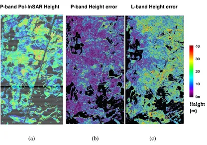
These properties are highlighted by Fig. 7, which shows the height and height error obtained from the inversion of single-baseline fully polarimetric ESAR Pol-InSAR data using the RVoG model for the Remningstorp test site. Note that this is the same scene as in Fig. 4. Fig. 7a shows the height map at P-band obtained from quasi-simultaneous acquisitions and is derived without using a priori information about terrain or vegetation density (Cloude & 460

Papathanassiou 2003, Hajnsek et al. 2009). Fig. 7b shows the corresponding height error at P-band obtained from acquisitions separated by 30 days. Biases introduced by temporal decorrelation are seen to be generally small (a few m) at P band, but can exceed 20 m at L band for the same temporal baseline (see Fig. 7c).

465

470 _{C L P}

Figure 6. Simulated effect on coherence of scatterer motions of RMS magnitudes 1, 3

and 5 cm as a function of wavelength, together with the range of wavelengths covered

by SAR systems operating at C-, L- and P-band.

475

P-band Pol-InSAR Height P-band Height error L-band Height error

(a) (b) (c)

Figure 7: (a) Height map derived from P-band Pol-InSAR for the Remningstorp test

site) Errors in estimates of height derived from 30-day coherence by Pol-InSAR

480

techniques at P- and L-band are shown in (b) and (c) respectively.

3.2.2 Allometric relations between biomass and forest height

The importance of height in estimating biomass comes from the key theoretical

relationship that, for a given species, the two are related by a power law:

485

α

H

where B is above-ground biomass and H is an estimate of height, and where variations

in the exponent

α

Equations of this form have been developed for trees in different forest zones, with

α

ranging from 0 to 4. For example, for four common European forest species (spruce,

490

pine, oak and beech), Mette (2007) found the relation

B = 0.801 × H1001.748 (3)

Where B is biomass in t ha -1, H100 denotes top height in metre, defined as the mean

height of the 100 trees with the largest diameter in a 1 ha area. For most forests, the

value of

α

495

should apply particularly to tropical forests, where the large variability of forest

attributes found for small plots is substantially reduced at a scale of 1 ha (Clark and

Clark 2000, Chave et al, 2001, Chave et al., 2003, Köhler & Huth, 1998).

The use of allometric equations to derive biomass from Pol-InSAR height will be

explored during Phase A of the mission; this will require further work to consolidate

500

allometric relationships for the major forest biomes.

3.2.3 Deriving forest information from SAR tomography

Phase 0 and Phase A include studies on the use of SAR tomography to gain information on

the interactions between radar waves and the forest canopies. This technique exploits

multi-baseline interferometric SAR observations to reconstruct the scattering from a vegetation

505

layer as a function of height (Reigber and Moreira (2000), Fornaro et al. (2005), Cloude, 2006; Tebaldini and Rocca, 2008). These measurements provide new insight into the physical

links between forest biomass and P-band observables, by clarifying the main P-band

scattering mechanisms in forest media, their relative contribution to the total radar signal,

and their variation over different forest types. Of particular value to the BIOMASS mission

is the ability of SAR tomography to distinguish the contributions to the radar signal from

the forest canopy (the tree crowns) and from double-bounce scattering, since the scattering

geometry causes the latter to appear as a return from ground level. Using the data acquired

at the Remningstorp forest, it was found that the relative contribution of the backscatter

from ground level is largely dominant for the HH and VV polarisations (the ratio is of the

515

order of 10 dB), and still dominant, though moderately, at HV (of the order of 3 dB)

(Tebaldini and Rocca, 2008, Tebaldini, 2010). Figure 8 shows the ratio between the

backscatter from the ground and from the canopy for HV polarisation (the same scene as

in figs. 4 and 7). The backscatter from the ground level was found higher than that of the

canopy level (corresponding to ground-to-canopy ratio >0 dB) in many of the forested

520

areas. This would not be expected from most current scattering models and indicates the

need for improved scattering models that take into account the impact of tree structure,

understorey and topography.

525

530

Figure 8: Ratio of the backscatter from ground level to the backscatter from canopy

level at HV with colour scale shown in dB. Non forest pixels are in black. The data are

from the same Remningstorp scene as in Figs. 4 and 7.

540

SAR tomography therefore leads to better understanding of which processes contribute

to the observed SAR signal, and should lead to both improved models of the interaction

between radar waves and the forest canopy, and better inversion methods using

intensity and Pol-InSAR. During the mission itself, it is proposed to further this process

by including a short experimental phase devoted to SAR tomography.

545

3.3. Exploiting intensity and Pol-InSAR information in biomass recovery

Section 3.1 shows the use of intensity data in biomass retrieval, while Sections 3.2.1

and 3.2.3 respectively illustrate the derivation of canopy height from Pol-InSAR and

the retrieval of information on forest structure from SAR tomography. It is of

considerable value that these independent types of information can be provided by the

550

same SAR system and combined in biomass retrieval, as is illustrated in Fig. 9 using

data from Remningstorp. Here the retrieval is based on linear regression of the mean

values of intensity, Pol-InSAR height and tomographic Ground to Volume backscatter

ratio derived from 10 reference plots of 80 m x 80 m, where accurate in situ biomass

measurements are available. The figure shows the comparison between estimated

555

biomass and in situ biomass for a) inversion of HV intensity data, b) inversion using

HV and HH intensity data together with Pol-InSAR height, and c) inversion using HV

and HH intensity data, Pol-InSAR height and the Ratio of Ground to Volume

into the inversion, going from 42.3 t ha-1 when using just HV intensity (comparable to

560

the inversion result in fig. 4, but with fewer test stands), to 27.9 t ha-1 with the addition

of HH and Pol-InSAR height, and to 11.0 t ha-1 when the tomographic HV ground to

canopy backscatter ratio is included. The result in 9c indicates that the structure

information provided by tomography enhances the information from Pol-InSAR height.

565

570

Figure 9: Comparison of estimated and in situ biomass for a) inversion of HV intensity

data, b) inversion using HV & HH intensity data together with Pol-InSAR height, and

c) inversion using HV & HH intensity data, Pol-InSAR height and the HV Ground to

Volume backscatter ratio. Squares: spruce stands, circles: pine stands, and triangles:

birch stands.

575

The inversion techniques are currently being tested on new airborne P-band datasets

acquired to assess two important effects: a) the impact of topography on backscatter

intensity and Pol-InSAR, and hence on biomass retrieval; this uses data acquired in

2008 from a boreal forest with marked topography; b) the temporal decorrelation in

tropical forests over time-intervals comparable with those for a spaceborne system

(20-580

45 days), using data acquired in French Guiana in 2009.

An important aim during the phase A studies is to provide better statistical

characterisation of the errors in the inversions. As can be seen from Fig. 2, these errors

RMSE= 42.28 t ha-1 _{RMSE= 27.93 t ha}-1 _{RMSE= 11.02 t ha}-1

are likely to depend on the biomass itself, as well as on issues such as system noise,

calibration errors and “geophysical” scatter arising from environmental perturbations of

585

the inversion relation. Joint error models are needed that take into account the different

measurements, such as intensity data and information derived from Pol-InSAR. This

information is important for quantifying not only the uncertainty in the estimated

biomass itself, but also how this propagates through carbon cycle estimates which make

use of it.

590

4 Measuring forest biomass change with time

Section 3 has focused on measuring biomass itself, which is of basic importance for

quantifying forest resources across the globe, but, as noted in Section 1, change in

forest biomass is the crucial variable needed for quantifying carbon fluxes and their

effects on climate.

595

The BIOMASS mission will address this by providing consistent and repeated global

observations of forests throughout the mission lifetime. These observations will

contribute to quantifying the dynamics of forest biomass in three ways:

1) From the time series of estimated biomass in all major forest biomes produced by

BIOMASS, the loss of biomass due to stand-removing disturbances can be easily

600

quantified.

2) The increase of biomass due to forest regrowth in the first years after disturbance can be

quantified at frequencies ranging from yearly to a single estimate over the whole 5-year

mission duration, depending on the forest biome, species and site index (or site quality). In

tropical forests, rates of growth can vary from 9 t ha-1 yr-1 to 21 t ha-1 yr -1 during the first

605

10 years of regrowth (Overman et al., 1994, Uhl et al., 1988), Such a differential rate of

areas. Conversely, for regions with very low recovery rate, the 5 year lifetime of

BIOMASS may not be sufficient. It is for example the case of Northern Eurasian forests in

regions with low site quality which may accumulate in the first years less than 1 t ha-1 yr-1

610

(IIASA 2007).

3) Detection and estimation of forest degradation due to selective removal of timber and

localised forest clearing requires the capability to detect changes in biomass in mature

forest stands. Analysis based on simulated 256-look HH and HV data in inversion indicates

that, except for the lowest levels of biomass, changes in biomass of around 30% are

615

detectable with error probability not exceeding 20% (European Space Agency, 2008).

5. Secondary mission objectives

Although the primary focus of the BIOMASS mission is the measurement of forest

biomass and its changes, this first chance to explore the Earth's environment with a

long wavelength satellite SAR provides major new geoscience opportunities. In

620

particular, BIOMASS is expected to provide new information on subsurface structure

in arid lands and polar ice, to extend existing information on forest inundation, and

potentially to provide information on quantities such as soil moisture, permafrost and

sea salinity.

5.1 Subsurface geomorphology

625

Low frequency SAR is able to map the subsurface down to several meters in arid areas,

thus has great potential for terrestrial applications, such as hydrology, geology, water

and oil resources, and archaeology (Abdelsalam et al., 2000), in arid and semi-arid

environments. In particular, the major drainage basins in North Africa are key features

for understanding climate change in the recent past, but are very poorly known.

630

Complete coverage of the eastern Sahara was provided by the Japanese JERS-1 L-band

northern Sudan, eastern Libya and northern Chad (Paillou et al., 2009). Such

continental-scale exploration is being continued with the PALSAR L-band radar on the

JAXA ALOS satellite. Its improved data quality has allowed mapping of a 1200

km-635

long palaeo-drainage system in eastern Libya that could have linked the Kufrah Basin

to the Mediterranean coast (Paillou et al., 2009). Such a major drainage system has

important implications for understanding the environments and climates of northern

Africa from the Late Miocene to the Holocene, with consequences for fauna, flora,

hominid and human dispersal.

640

These promising results from L-band are likely to be considerably improved by the

increased penetration offered at P-band. Using values of dielectric constant that are

typical for dry sandy sediments, an L-band SAR would have an expected penetration

depth of about 1.3 m, while P-band should penetrate to about 3.7 m. Aircraft campaigns

have in fact demonstrated that P-band SAR can penetrate to at least 4 m in sandy

645

environments (Farr, 2001; Grandjean et al., 2001).

5.2 Sub-surface ice structures and interferometric ice flow measurements

A limitation of shorter wavelength SAR systems (e.g. C-band) for ice studies is their

lack of penetration into ice, together with the fact that surface change processes can

produce a loss of coherence in interferometric data. It is expected that the P-band signal

650

will penetrate tens of metres of ice, thus reaching larger and more stable scatterers deep

under the ice surface. This not only means that subsurface structure can be investigated,

but also that interferometric coherence over ice should remain high, allowing the

monitoring of glacier displacements over longer time than can be achieved with

interferometry at higher frequencies (Mattar et al., 1998, Rignot et al., 2008). A P-band

655

valuable information about glacier dynamics over periods that correspond to annual

change.

5.3 Forest inundation

A basic requirement for modeling methane or carbon dioxide emissions from inundated

660

forests is information on the spatial and temporal distributions of inundated area. The

ability of long wavelength radar to map wetland inundation (for example, the Amazon

and the Congo basins) has been demonstrated using JERS L-band data (Hess et al.,

2003, Martinez and Le Toan, 2007). Using ALOS PALSAR, the timing and duration of

flooding over entire catchments have been spectacularly displayed (see

665

http://www.eorc.jaxa.jp/ALOS/kyoto/jan2008/pdf/kc9_hess.pdf). Systematic data

acquisition over all the inundated forest areas and the greater penetration into the forest

canopy by the BIOMASS sensor mean that it will add substantially to the time-series

being produced by PALSAR and allow the study of decadal trends and inter-annual

variations in the dynamics of these very important ecosystems.

670

6. Mission characteristics

The science requirements of the BIOMASS mission place strong constraints on the

characteristics of the space segment. These are briefly discussed in this Section, which

pulls together many of the ideas set out in previous sections. A summary is also given

in Table 1, and a more complete treatment will be found in the BIOMASS Report for

675

Assessment (European Space Agency, 2008).

Polarimetry. Access to the full range of biomass encountered in the world’s forests

requires measurement of forest height, and hence a fully polarimetric system in order to

support polarimetric interferometry. In addition, direct methods of measuring forest

biomass benefit from using intensity measurements at multiple polarisations, and

correction of Faraday rotation caused by the ionosphere requires polarimetric data

(Bickel and Bates, 1965; Freeman, 2004; Qi and Jin, 2007; Chen and Quegan, 2009).

Resolution. Two considerations underlie the choice of resolution of the BIOMASS

sensor. The first is scientific, and is the need to make measurements at a scale

comparable to that of deforestation and forest disturbance, i.e. around 1 ha. The second

685

is forced by the ITU allocation of only 6 MHz to P-band for remote sensing, which

corresponds to a ground range resolution of around 50 m (depending on the incidence

angle). It is envisaged that BIOMASS will provide level-1 products with around 50 m x

50 m resolution at 4 looks. By applying optimal multi-channel filtering techniques to a

time-series of HH, HV and VV intensity data, the speckle in each image can be

690

significantly reduced without biasing the radiometric information in each image. For

example, a multi-temporal set of six such triplets of intensity data would yield an

equivalent number of looks of around 40 or greater at each pixel (Quegan and Yu,

2001), so averaging 2x2 blocks of pixels would yield around 150 looks at a scale of 1

ha, after allowing for inter-pixel correlation. This yields a radiometric accuracy better

695

than 1 dB, which is sufficient to meet the science objectives.

Incidence angle. Airborne experiments have been carried out for incidence angles ranging

from 25° to 60°, and most indicate that the preferred incidence angle is in the range

40-45°.However system considerations are expected to favour steeper incidence angles. Currently, the minimum incidence angle is set to >23 degrees. Until now, the effect of incidence angles is not 700

thoroughly addressed. In a study on the sensitivity of the SAR intensity (HV) to biomass (Dubois-Fernandez et al., 2005), similar γ backscatter coefficients were obtained at 23° and at 40° for biomass higher than 50 t ha-1, whereas for lower biomass, the backscatter signal is higher at 23°. This is in line with current research based on airborne SAR tomography (Cf. Section 3.2.3) which suggests that observations at incidence angles of 20°-30° may increase the

volume ratio, in particular for sparse forests and forests in regions with relief, hence

increasing the error in biomass retrieval based only on HV intensity. In this case,

algorithms based on a combination of different SAR measurements are required.

Quantitative assessment of the effect of incidence angle on the SAR intensity, SAR

polarimetry, and on PolInSAR and tomography is currently undertaken in the mission

710

phase A, aiming at consolidating the choice of incidence angle and at improving the

retrieval algorithms.

Revisit time. Forest height recovery using Pol-InSAR requires a revisit time small

enough to maintain high temporal coherence between successive SAR acquisitions.

Although this issue is still being investigated, preliminary results suggest that a time

715

interval of between 25-45 days is acceptable.

Orbit. A sun-synchronous dawn-dusk orbit will minimise ionospheric disturbances

(Quegan et al., 2008).

Mission duration. A 5-year mission is planned in order to obtain repeated

measurements of the world’s forests. This will lead to reduced uncertainties in

720

measurements of the biomass of undisturbed forests and will allow measurement of

forest dynamics by detecting changes in biomass and forest cover. Although the

regrowth of fast-growing tropical forests may be detectable even with measurements

spaced one or two years apart, measurement of regrowth in temperate forests requires

as long a mission as possible. BIOMASS will have very limited capability for

725

measuring regrowth in the slowly-growing boreal forests.

Tomography. The mission is expected to include a short tomographic phase during

which measurements with 10-12 spatial baselines and a revisit time of 1-4 days will be

7. Summary and Conclusions 730

At present, the status, dynamics and evolution of the terrestrial biosphere are the least

understood and the most uncertain elements in the global carbon cycle, which is deeply

imbedded in the functioning of the Earth system and its climate. There are very large

uncertainties in the distribution of carbon stocks and carbon exchange, in the estimates

of carbon emissions due to land use change, and in the uptake of carbon due to forest

735

regrowth. Forest biomass is the main repository of vegetation carbon and hence is a

crucial quantity needed to reduce these uncertainties. Both its spatial distribution and its

change with time are critical for improved knowledge of the terrestrial component of

the carbon cycle.

Although the need is great and urgent, there are no current biomass datasets that are

740

global, up-to-date, consistent, at spatial resolutions comparable with the scales of land

use change, or that are systematically updated to track biomass changes due to land use

change and regrowth. The BIOMASS mission is designed to address this severe

limitation in our knowledge of the Earth and its functioning. It will aid in building a

sustained global carbon monitoring system that improves over time, thus helping

745

nations to quantify and manage their ecosystem resources, and to improve national

reporting. Its value will also extend well beyond the mission lifetime: since biomass in

undisturbed forest changes relatively slow, the maps produced during the mission will

provide realistic values for calculations of emissions based on deforestation maps

produced by other means, such as optical or shorter wavelength radar sensors.

750

The design of the BIOMASS mission is driven by science needs, and spins together two

main observational strands: (1) the long heritage of airborne observations in tropical,

temperate and boreal forest that have demonstrated the unique capabilities of P-band

developments in recovery of forest height from Pol-InSAR, and, crucially, the

755

resistance of P-band to temporal decorrelation, which makes this frequency uniquely

suitable for biomass measurements with a single repeat-pass satellite. These two

complementary measurement approaches are combined in the single BIOMASS sensor,

and have the satisfying property that increasing biomass reduces the sensitivity of the

former approach while increasing the sensitivity of the latter. During phase A of the

760

mission, the inversion methods are consolidated using new experimental data acquired

over forests with marked topography and over forests with very high biomass density.

However, the BIOMASS P-band radar appears to be the only sensor capable of

providing the urgently needed global knowledge about biomass. It seizes the new

opportunity from the allocation of a P-band frequency band for remote sensing by the

765

ITU in 2003. It also will be a major addition to current efforts to build a global carbon

data assimilation system (Ciais et al., 2003) that will harness the capabilities of a range

of satellites and in situ data. It is within this context that BIOMASS will find its fullest

expression, both gaining from and complementing what can be learnt from other

satellite systems, ground data, and carbon cycle models.

770

References

Abdelsalam, M. G., Robinson, C., El-Baz, F., & Stern, R. J. (2000). Applications of

orbital imaging radar for geologic studies in arid regions: The Saharan testimony.

775

Photogrammetric Engineering and Remote Sensing, 66, no. 6, 717-726.

780

Askne, J., Dammert, P. B., Ulander, L. M., & Smith, G. (1997). C-Band repeat-pass

interferometric SAR observations of the forest. IEEE Transactions on Geoscience and

Remote Sensing, 35, no. 1, 25-35.

Beaudoin, A., Le Toan, T., Goze, S., Nezry, E., Lopes, A, et al. (1994). Retrieval of

785

forest biomass from SAR data. International Journal of Remote Sensing, 15, 2777-2796.

Beer, C., Lucht, W., Schmullius. C., & Shvidenko, A. (2006). Small net uptake of

carbon dioxide by Russian forests during 1981-1999. Geophysical Research Letters,

33: L15403-doi:10.1029/2006GL026919.

790

Bickel, S. H. and Bates, R. H. T. (1965). Effects of magneto-ionic propagation on the

polarization scattering matrix. Proc. IRE, vol. 53, 1089-1091.

Bunker, D. E.,DeClerck, F., Bradford, J. C., Colwell, R. K., Perfecto, I., et al. (2005).

795

Species loss and aboveground carbon storage in a tropical forest. Science, 310, no. 5750,

1029-1031.

Canadell, J. G., Le Quéré, C., Raupach, M. R., Field, C.B, Buitehuis, E. T., et al. (2007)

Contributions to accelerating atmospheric CO2 growth from economic activity, carbon

800

intensity, and efficiency of natural sinks. Proceedings of the National Academy of

Science, 104, 18866–18870.

Ciais, P., Moore, B., Steffen, W., Hood, M., Quegan, S., et al. (2003). Final Report on

Strategy to Build a Coordinated Operational Observing System of the Carbon Cycle

805

and its Future Trends, FAO.

Chave, J., Riéra, B., & Dubois, M.A. (2001). Estimation of biomass in a neotropical

forest of French Guiana: spatial and temporal variability. Journal of Tropical Ecology,

17, 79-96.•

Chave,J, Chust,G., Condit R., Aguilar S., Lao S., Perez R. 2004. Error propagation and scaling

810

for tropical forest biomass estimates. Philosophical Transactions of the Royal Society of

London B 359, 409-420.

Chave, J., Condit, R., Lao, S., Caspersen, J. P., Foster, R. B., et al. (2003). Spatial and

temporal variation in biomass of a tropical forest: results from a large census plot in

815

Panama. Journal of Ecology, 91, 240-252.

Chen, J. and Quegan, S. (2009). Improved estimators of Faraday rotation using

spaceborne polarimetric SAR data. IEEE Trans. Geosci. Remote Sens. Letts. (under

review).

Clark, D. B. & Clark, D. A. 2000 Landscape-scale variation in forest structure and biomass in a 820

tropical rain forest. ForestEcol. Mngmt 137, 185–198.

Cloude, S. R. & Papathanassiou, K. P. (1998). Polarimetric SAR interferometry. IEEE

Transactions on Geoscience and Remote Sensing, 36, no. 5, 1551-1565.

Cloude, S. R., Papathanassiou, K. P. & Pottier, E. (2001). Radar polarimetry and

polarimetric interferometry. IEICE Transactions on Electronics, E84-C, no. 12,

1814-825

1822

Cloude, S. R. (2006). Polarisation coherence tomography. Radio Science, 41, RS-4017.

Dubois-Fernandez, P., Champion, I., Guyon D., Cantalloube H., Garestier F., Dupuis

X., Bonin G., Forest biomass estimation from P-band high incidence angle data.