White Rose Research Online URL for this paper:
http://eprints.whiterose.ac.uk/76527/
Version: Accepted Version
Article:
Stannett, M.P. orcid.org/0000-0002-2794-8614 and Németi, I. (2013) Using Isabelle/HOL
to verify first-order relativity theory. Journal of Automated Reasoning, 52. pp. 361-378.
ISSN 0168-7433
https://doi.org/10.1007/s10817-013-9292-7
[email protected] https://eprints.whiterose.ac.uk/
Reuse
Unless indicated otherwise, fulltext items are protected by copyright with all rights reserved. The copyright exception in section 29 of the Copyright, Designs and Patents Act 1988 allows the making of a single copy solely for the purpose of non-commercial research or private study within the limits of fair dealing. The publisher or other rights-holder may allow further reproduction and re-use of this version - refer to the White Rose Research Online record for this item. Where records identify the publisher as the copyright holder, users can verify any specific terms of use on the publisher’s website.
Takedown
If you consider content in White Rose Research Online to be in breach of UK law, please notify us by
(will be inserted by the editor)
Using Isabelle/HOL to verify first-order relativity theory
Mike Stannett · Istv´an N´emeti
August 22, 2013
Abstract Logicians at the R´enyi Mathematical Institute in Budapest have spent several years developing versions of relativity theory (special, general, and other variants) based wholly on first-order logic, and have argued in favour of the physi-cal decidability, via exploitation of cosmologiphysi-cal phenomena, of formally unsolvable questions such as the Halting Problem and the consistency of set theory. As part of a joint project, researchers at Sheffield have recently started generating rigorous machine-verified versions of the Hungarian proofs, so as to demonstrate the sound-ness of their work. In this paper, we explain the background to the project and demonstrate a first-order proof in Isabelle/HOL of the theorem “no inertial ob-server can travel faster than light”. This approach to physical theories and physical computability has several pay-offs, because the precision with which physical the-ories need to be formalised within automated proof systems forces us to recognise subtly hidden assumptions.
Keywords Isabelle/HOL · first-order relativity theory · hypercomputation ·
physics and computation
CR Subject Classification F.4.1·J.2
1 Introduction
The Hungarian team of Andr´eka et al. have formalised a series of relativity theories (including special and general relativity) using order logic [1, 2]. These first-order foundations ensure that their theories are easy to reason with, but also introduce a number of nonstandard features. This school uses the intuition-friendly and logically benign framework of first-order logic for formalizing and elaborating
M. Stannett
Department of Computer Science, University of Sheffield Regent Court, 211 Portobello, Sheffield S1 4DP, United Kingdom, Tel.: +44-114-2221800, Fax: +44-114-2221810, E-mail: [email protected],
I. N´emeti
relativity theories. However, their proofs are often formulated in the intuitive, informal language of model theory (as opposed to proof theory). Therefore, a theoretical doubt may arise whether these proofs can always be pushed through on the purely syntactical (i.e., proof theoretical) level. We have, therefore, recently started a joint project verifying their theories using the Isabelle proof assistant [3]. We explain our approach below, and outline an Isabelle/HOL proof of the well-known statement “no inertial observer can travel faster than light” [4, 5].
While the initial encoding of the underlying axioms within Isabelle/HOL is essentially straightforward, automating the proof proved unexpectedly challenging. In Sect. 2 we explain the logical foundations of the proof construction, and show how the axiom systems are encoded in Sect. 3. The proof itself is presented in Sect. 4, and follow-on questions are discussed in Sect. 5.
An example of a situation where the correctness of a relativity theoretic proof can be challenging is the following. In his seminal analysis of computation, Turing [6] discussed the nature of human computation, and showed that certain tasks – most famously, the Halting Problem (HP) – are not decidable by computational means. Subsequent theoretical investigation by various researchers suggests, how-ever, that physical systems may exist which can in fact decide HP by exploiting cosmological phenomena [7–12]. We focus here on one particular scheme for cos-mological hypercomputation [9, 13], and consider the extent to which it rests on secure logical foundations. Doing so we can rely on the above described FOL ax-iomatic foundations of relativity theories. We return to this question in more detail in Sect. 5.
2 Logical foundations
The statement we wish to prove (“no inertial observer can travel faster than light”) says that when one inertial observer,m, sees another,k, at two distinct spacetime locationseand f, the latter cannot be spacelike separated (see Sect. 4). To prove this statement we turn to Andr´eka et al.’s [1, 5] first-order formalisation of relativ-ity theory. Our focus on first-order logic (FOL) is motivated by several important considerations. Foremost is the Hungarian team’s desire to demystify relativity theory by expressing its postulates and conclusions in a form that is intelligible to as large an audience as possible. By choosing simple language and a very simple axiom system, the underlying assumptions of the theory are made as straightfor-ward as possible (see Sect. 3.2), while the use of first-order logic and its simple reliance on Modus Ponens makes it relatively easy for newcomers to follow the proofs. Having reformulated relativity in purely logical terms, the group is also able to investigate which axioms underpin which results and which are superflu-ous. Given the physical nature of the theory in question, this information can then be reflected back into physics: if an axiom plays no role in establishing an experi-mentally observed result, then that result can neither support nor undermine the validity of the axiomatic property in question.
like the existence of suprema of bounded sequences, are unavailable in a rigorous first-order logical proof (this existence condition is called theContinuity Axiom in the mathematical and logical literature).1
In particular, the statement that any decreasing sequence of real numbers, bounded below, has a greatest lower bound is not a first-order statement, because it refers to orderedsets of real values.2
More-over, as Andr´eka and her colleagues have shown, many interesting theorems for relativity can be proven using less restrictive fields like the rationals,Q, for which the real-number propertyevery positive number has a positive square rootfails3
(such fields are said to benon-Euclidean), cf. [14].
2.1 The need for formal verification
Given that “first-order numbers” need not exhibit the properties typically expected of them by physicists, it is important that we treat traditional explanations of relativistic phenomena with caution. To this end, as part of a Royal Society Inter-national Exchanges Scheme project, researchers in Sheffield joined forces with the Hungarian team at the start of 2012, to develop a comprehensive formal frame-work for relativity theory, with full machine-verification of all derived theorems. To the best of our knowledge, this is the first time such a large-scale physical theory has been treated in this way (but cf. [15, 16]), and it is hoped that the lessons learned will be useful in extending the approach more widely. The project has been planned in four main stages, and it is hoped that the end result will be a formal machine-verified proof of the controversial claim that the power of a computational system depends on the nature of its spacetime environment, with super-Turing capabilities emerging in the context of more complex spacetime ge-ometries.
The project itself has four broad aims:
Goal 1. Implement first-order axiomatizations of general relativity using the
proof assistant Isabelle [3];
Goal 2. Add a general model of computational mobility to the theory, to enable
the modelling of computations carried out by machines travelling along specific spacetime trajectories;
Goal 3. Consider how the power of these computational systems changes
ac-cording to the underlying topology of spacetime [17];
Goal 4. Select a recursively uncomputable problemP(for example, the Halting Problem) and machine-verify the following claims:
(a) in simpler relativistic settings,Premains uncomputable; (b) in some spacetimes,Pcan be solved.
1
For completeness, we note that this difficulty can be solved within FOL in many ways, e.g., it can be solved by focussing attention on definable sets.
2
There are fields which have the same first-order properties asR, but which contain infinites-imals. In such a field, the bounded decreasing sequence 1
1> 1 2>
1
3> . . . has no greatest lower bound. For supposeαwere its greatest lower bound; then given any positive infinitesimalǫ, the value (1 +ǫ)αwould be a slightly larger lower bound, thereby contradicting the definition ofα.
3
Taken together, these steps are intended to add weight to the claim that the computational power of a device may depend on the physical setting in which it finds itself.
3 The theories and their implementation
There are various versions of relativity theory, depending on what is being mod-elled. For special relativity (SpecRel) the two key axioms (suitably formalised)
are [4]:
Principle of relativity:The laws of nature are the same for every inertial observer;
Light postulate: Any ray of light moves in the ‘stationary’ system of co-ordinates with the determined velocityc, whether the ray be emitted by a stationary or by a moving body;
while for general relativity (GenRel) we add the
Equivalence Principle: It is not possible to distinguish locally between the effects of acceleration and those of gravity.
In addition to special and general relativity, Sz´ekely and his colleagues have made a detailed study ofaccelerated observers(with or without the equivalence prin-ciple in place). The corresponding theory,AccRel, provides a convenient stepping
stone from special to general relativity [14]. Our Isabelle implementation4
has been constructed in three parts, a pro-gram structure that ensures that different versions of relativity theory can eas-ily be added later. For example, to add GenRelwe would simply add a new file GenRel.thywhich merges the required axiom classes and includes proofs of relevant theorems. We focus here on the first-order theory SpecRel of special relativity.
This theory is 2-sorted, the sorts being Quantities (the values used to specify coordinates, speeds, masses, etc) andBody(bodies ortest particles).
3.1 Background geometry (SpaceTime.thy, approx. 830 lines)
This Isabelle/HOL code file models the geometric structures common to all models of spacetime (Vectors,Points,Lines,Planes,Cones), each represented as a sepa-rate record structure with axioms attached. The axioms describe basic geometric relationships including, for example, what it means for three points to be collinear, what it means for two vectors to be orthogonal, and so forth. In particular, a key lemma for our main proof is the assertion that distinct parallel lines cannot meet (the proof is by contradiction). Having defined these classes, we takeSpaceTimeto be their conjunction:
class SpaceTime = Quantities + Vectors + Points + Lines + Planes + Cones
4
The set of Quantitiesis assumed to carry an ordered field structure. We shall sometimes need to assume that the field is also Euclidean – i.e., that square roots exist for positive values – but this is not a general requirement, so it will be added as a separate axiom class later. Since Isabelle/HOL already includes a suitable class, the implementation of Quantitiesis particularly simple:
class Quantities = linordered_field
For simplicity we assume that spacetime is (1 + 3)-dimensional (one time di-mension + three space didi-mensions), so thatPointsandVectorsare both specified as 4-tuples of Quantities. In more complex relativity theories, we allow both the number of space dimensions, and the number of time dimensions, to range over arbitrary positive integers. Lines are specified by giving a point (the line’s base-point) and a vector (its direction), while planes are specified by a basepoint and two vectors. These formalisations are not unique with respect to the underlying abstract pointsets they are intended to represent (for example, there are infinitely many representations of each line, because we can choose any of its points as base-point), but in practice this makes no difference, since all relevant functions remain well-defined.
Because we are dealing here with special relativity, all lightcones can be consid-ered to be ‘upright’ (for general relativity we need to allow cones that are ‘tilted’ by curvature effects); each cone can therefore be specified by giving a point (its
vertex) and a quantity (itsslope). However, the freedom with which we can specify quantities has certain concomitant side-effects, and these need to be taken into account. In real-number physics, we would consider the slope of the cone
x2+y2+z2=αt2 whereα >0
to be√α, but whenQuantitiesis non-Euclidean we cannot be certain that√αis defined. Consequently, we take the slope of the cone to beαrather than√α, and adjust all associated formulae and proofs accordingly.
3.2 Axioms (Axioms.thy, approx. 260 lines)
This file includes various axioms used by the Hungarian group, each implemented as a separate class. Different relativity theories can then be constructed by merging the relevant axiom classes and omitting those that are not required; we focus here on the axioms that will be needed to specify SpecRel.
The axioms describe the events in which bodies can participate, and how their descriptions change from one observer’s viewpoint to another. Here, a Body can be either aphoton (which always travels at constant speed) or aninertial observer
(which always travels at constant speed, and in addition is capable of making observations). Since we do not assume a priori that the classes of photons and inertial observers are disjoint, we represent bodies using an Isabelle/HOL record structure:
At first sight, this formalisation appears slightly odd, since it suggests the possibility of four types of body (one which is neither photon nor inertial observer, one which is purely a photon, one which is purely an inertial observer, and one which is both at the same time), but in keeping with our goal of placing as few restrictions as possible on the underlying theory, we have resisted the temptation to separate out photons from inertial observers a priori (e.g. by specifying them using distinct type variables in a locale). Instead, we note that such type confusions can never actually occur, since it is a theorem, for example, that no object can be simultaneously a photon and an inertial observer (according to our axioms, inertial observers see themselves as stationary in space, while photons have no choice but to move at lightspeed, which is strictly positive; the two are clearly incompatible). For more complex relativistic theories we also need to consider non-inertial observers (those which can accelerate), as well as more general types of body, and in this regard the use of Isabelle/HOL record structures is particularly convenient, since we can easily extend the Bodyrecord structure to include new descriptions (once again, we can prove from the axioms introduced to describe these bodies that no type confusions arise when we do so). The distinction between inertial observers and more general body types emerges in these more advanced theories. For example, we demonstrate below that inertial observers can never travel faster than (what they consider to be) the speed of light, but this property neednot be provable of more general bodies [18, 19].
In addition to the ordered field axioms associated withQuantities,SpecRelis formally generated using just the four axioms described below (AxPh,AxEv,AxSelf,
AxSym), but in practice we have found it sensible to replaceQuantitieswith a larger
WorldView class (below) so as to have available the necessary abbreviations and functions. This simplifies proofs considerably. Moreover, our proof that inertial observers cannot travel faster than light requires us to find the intersection of a line with a cone, and this in turn requires the existence of square roots – we have therefore included the Euclidean axiom (AxEuclidean). Finally, we make use of various additional properties of cones, lines and planes (given inSpaceTime.thy). These define various relatively complicated concepts, such as what it means for a plane to be tangent to a (light)cone:
class Cones = Quantities + Lines + Planes + fixes
tangentPlane :: "’a Point ⇒ ’a Cone ⇒ ’a Plane"
assumes (* The basepoint of the tangent-plane-at-e is e *) AxTangentBase: "pbasepoint (tangentPlane e cone) = e"
and (* The tangent plane contains the vertex *)
AxTangentVertex: "inPlane (vertex cone) (tangentPlane e cone)"
and (* The tangent plane meets the cone in a line *) AxConeTangent: "(onCone e cone) −→
(inPlane pt (tangentPlane e cone) ∧ onCone pt cone) ←→ collinear (vertex cone) e pt)"
in that plane, and the intersection lines are parallel. *) AxParallelCones: "(onCone e econe ∧ e 6= vertex econe
∧ onCone f fcone ∧ f 6= vertex fcone ∧ inPlane f (tangentPlane e econe))
−→ (samePlane (tangentPlane e econe) (tangentPlane f fcone)
∧ ((lineJoining (vertex econe) e) k (lineJoining (vertex fcone) f)))"
and (* If f is outside a cone, there is a tangent plane to that cone which contains f. The tangent plane is determined by some e lying on the intersection line with the cone. *)
AxParallelConesE: "outsideCone f cone −→ (∃e.(onCone e cone ∧ e 6= vertex cone ∧ inPlane f (tangentPlane e cone)))"
3.2.1 Square roots
TheEuclidean field axiom,AxEuclidean, states that every positive quantity has a
positive square root, and defines thesqrtfunction.
class AxEuclidean = Quantities + assumes
AxEuclidean: "(x ≥ (0::’a)) =⇒ (∃r. ((r ≥ 0) ∧ (r*r = x)))" begin
fun sqrt :: "’a ⇒ ’a" where
"sqrt x = (SOME r. ((r ≥ (0::’a)) ∧(r*r = x)))" end
In keeping with our policy of keeping the axioms as unrestrictive as possible, we do not assume that the positive square root is uniquely defined, though this is, of course, an easy theorem.
3.2.2 The WorldView relation
Two key features of first-order relativity theory are theworldview relation (W) and theworldview transformation (wvt).
class WorldView = SpaceTime + fixes
(* Worldview relation *)
W :: "Body ⇒ Body ⇒ ’a Point ⇒ bool" (" sees at ") and
(* Worldview transformation *)
wvt :: "Body ⇒ Body ⇒ ’a Point ⇒ ’a Point" assumes
AxWVT: "J IOb m; IOb k K=⇒ (W k b x ←→ W m b (wvt m k x))" and
end
The relationWtells us which bodies an inertial observermsees at each space-time location. Thus,W m b pisTrueprecisely whenmconsiders the body (whether inertial observer or photon)bto be present at locationp. We can useWto define various standard concepts; for example, the worldline of b(fromm’s point of view) is simply the set{p . W m b p}.
The worldview transformation tells us how one observer’s viewpoint is related to another. AsAxWVTexplains, if wvt m k xisy, this means that whatever ksees atx,msees aty.
3.2.3 Photons and the speed of light
Thephoton axiom,AxPh, says that for any inertial observer, the speed of light (c)
is the same in every (spatial) direction everywhere and is positive. Furthermore, it is possible to send out a light signal in any (spatial) direction. (The auxiliary functions space2 and time2 give the squared spatial and temporal separations, respectively, of two spacetime locationsxand y.)
class AxPh = WorldView + assumes
AxPh: "IOb(m)
=⇒ (∃v. ( (v > (0::’a)) ∧ ( ∀x y . ( (∃p. (Ph p ∧ W m p x ∧ W m p y))
←→ (space2 x y = (v * v)*(time2 x y)) ))))"
begin
fun c :: "Body ⇒ ’a" where
"c m = (SOME v. ( (v > (0::’a)) ∧ ( ∀x y . ( ∃p. (Ph p ∧ W m p x ∧ W m p y))
←→ (space2 x y = (v * v)*(time2 x y)) )))"
fun lightcone :: "Body ⇒ ’a Point ⇒ ’a Cone" where lightcone m v = mkCone v (c m)"
(* various lemmas follow that are not included here *)
3.2.4 Events
The event axiom, AxEvent, says that all inertial observers are participating in
the same universe – if one observer sees two bodies meeting at some spacetime location, they all see them meeting (though they may disagree as to where and when that meeting takes place).
class AxEv = WorldView + assumes
AxEv: "J IOb m; IOb k K =⇒ (∃y. (∀b. (W m b x ←→ W k b y)))" begin
end
3.2.5 Self-observation
The self axiom, AxSelf, says that inertial observers consider themselves to be
stationary in space (so they consider their worldline to be the time axis).
class AxSelf = WorldView + assumes
AxSelf: "IOb m =⇒ (W m m x) −→ (onAxisT x)" begin
end
3.2.6 Spatial calibration
The symmetry axiom, AxSym, says that inertial observers agree as to the
spa-tial distance between two spacetime events if these two events are simultaneous for both of them. This is essentially an auxiliary axiom, explaining how inertial observers calibrate their measuring rods to allow comparison of measurements.
class AxSym = WorldView + assumes
AxSym: "J IOb m; IOb k K =⇒
(W m e x ∧ W m f y ∧ W k e x’ ∧ W k f y’ ∧ tval x = tval y ∧ tval x’ = tval y’ ) −→ (space2 x y = space2 x’ y’)"
begin end
3.3SpecRel(SpecRel.thy, approx. 340 lines)
This file defines the theorySpecRel. The theory is remarkably sparse, being based
class SpecRel = WorldView + AxPh + AxEv + AxSelf + AxSym (*
The following proof assumes that the quantity field is Euclidean. *)
+ AxEuclidean (*
We also assume for now that lines, planes and lightcones are preserved by the worldview transformation. This can be proven. *)
+ AxLines + AxPlanes + AxCones
4 The proof
We have formalised the statement “no inertial observer can travel faster than light” as:
lemma noFTLObserver: assumes iobm: "IOb m" and iobk: "IOb k" and mke: "m sees k at e" and mkf: "m sees k at f" and enotf: "e 6= f"
shows "space2 e f ≤ (c m * c m) * time2 e f"
To see why, notice that the statement “kcannot travel faster than light” is mean-ingless as it stands. We need to sayin whose opinion this statement is true, since speeds depend on the observer. We therefore have to introduce a second inertial observer, m, in whose opinion the judgment is to be made. To find the speed at which kis moving, m needs to observe k at two different locations,e and f, and then determine the (square of the) ratio of the associated spatial and temporal separations.
The proof itself is in five basic stages.
Step 1. Assume the converse
Supposekis going faster than light (FTL) fromm’s viewpoint:
assume converse: "space2 e f > (c m * c m) * time2 e f"
Informally, we are saying thatflies outsidem’s lightcone ate.
Step 2. Consider the cone ate
def eCone ≡ "mkCone e (c m)"
have e on econe: "onCone e eCone" by (simp add: eCone def)
Step 3. Identify the tangent plane containingf
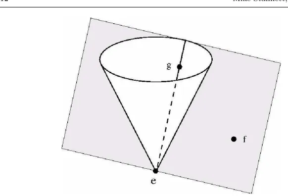
Step 1 tells us to assume thatfis outside the cone. We can use the cone axioms to find a tangent plane containing f. Being a tangent plane, it will necessarily contain the vertex,e, as well. In addition, the axioms allow us to fix a pointg so that the line joining gto the vertex is the line of intersection between the cone and the tangent plane. Notice thatg is distinct from botheand f, and together the three points define the tangent plane (Fig. 1).
have e is vertex: "e = vertex eCone" by (simp add: eCone def) have cm is slope: "c m = slope eCone" by (simp add: eCone def) hence outside: "outsideCone f eCone"
by (metis (lifting) e is vertex cm is slope converse outsideCone.simps)
have "outsideCone f eCone
−→ (∃x.(onCone x eCone ∧ x 6= vertex eCone ∧ inPlane f (tangentPlane x eCone)))" by (rule AxParallelConesE)
hence tplane exists: "∃x.(onCone x eCone ∧ x 6= vertex eCone ∧ inPlane f (tangentPlane x eCone))"
by (smt outside)
then obtain g where g props: "(onCone g eCone ∧ g 6= vertex eCone ∧ inPlane f (tangentPlane g eCone))"
by auto
have g on eCone: "onCone g eCone" by (metis g props) have g not vertex: "g 6= vertex eCone" by (metis g props) (* ... and more ... *)
Step 4. Switch tok’s viewpoint
Because m sees k at the distinct points e and f, k should also see itself at (its transformed versions of) those points, byAxEv. But each observer considers itself to be stationary, so k considers e and f to be distinct points on his time axis, by AxSelf. If k’s worldline also passed throughg, the pointse, fandg would be collinear ink’s worldview, and hence also in m’s, and we know this not to be the case because eand g are both in the tangent intersection line, whilefis outside the cone. Consequently,gis not onk’s time axis.
Fig. 1 Given a light cone with vertexeand a pointf outside the cone, we can find a plane that containsf and which is tangent to the cone. We choosegto be any point (apart frome) which lies on the line of intersection between the plane and the cone.
def wvtf ≡ "wvt k m f" def wvtg ≡ "wvt k m g"
have "W k k wvte" by (metis wvte def AxWVT mke iobm iobk) hence wvte onAxis: "onAxisT wvte" by (metis AxSelf iobk)
have "W k k wvtf" by (metis wvtf def AxWVT mkf iobm iobk) hence wvtf onAxis: "onAxisT wvtf" by (metis AxSelf iobk)
have wvte inv: "e = wvt m k wvte" by (metis AxWVTSym iobk iobm wvte def) have wvtf inv: "f = wvt m k wvtf" by (metis AxWVTSym iobk iobm wvtf def) have wvtg inv: "g = wvt m k wvtg" by (metis AxWVTSym iobk iobm wvtg def)
have e not g: "e 6= g" by (metis e is vertex g not vertex)
have f not g: "f 6= g" by (metis outside lemOutsideNotOnCone g on eCone) have wvt e not f: "wvte 6= wvtf" by (metis wvte inv wvtf inv enotf) have wvt f not g: "wvtf 6= wvtg" by (metis wvtf inv wvtg inv f not g) have wvt g not e: "wvtg 6= wvte" by (metis wvtg inv wvte inv e not g) have if g onAxis: "onAxisT wvtg −→ collinear wvte wvtg wvtf"
by (metis lemAxisIsLine wvte onAxis wvtf onAxis wvt e not f wvt f not g wvt g not e)
[image:13.595.72.363.73.271.2]hence wvtg offAxis: "¬ (onAxisT wvtg)" by (metis g not collinear)
Step 5. Find a pointzwith impossible properties
We have seen thateandfdefine the time axis (fromk’s point of view), andglies off this axis. Consequently, because all lightcones are upright in special relativity, the line joininge tog has non-empty intersection with thek-lightcone atf. Call the point of intersection z, and observe that thek-lightcone at zcontains bothe
andf. [Notice, however, that determining the coordinates of the pointztypically involves the use of square roots, which is why we have assumedAxEuclidean.]
Having obtainedz, we will prove that its properties are contradictory.
have "∀s.(∃p.( collinear wvte wvtg p
∧ (space2 p wvtf = (s*s)*time2 p wvtf)))" by (metis lemSlopedLineInVerticalPlane
wvte onAxis wvtf onAxis wvtg offAxis wvt e not f) hence exists wvtz: "∃p.( collinear wvte wvtg p
∧ (space2 p wvtf = (c k * c k)*time2 p wvtf))" by metis
then obtain wvtz where
wvtz props: "collinear wvte wvtg wvtz
∧ (space2 wvtz wvtf = (c k * c k)*time2 wvtz wvtf)" by auto hence wvtf speed: "space2 wvtz wvtf = (c k * c k)*time2 wvtz wvtf"
by metis
def z ≡ "wvt m k wvtz"
We know that f is on k’s lightcone at z, and that lightcones are mapped to lightcones under worldview transformations. We can therefore switch to m’s viewpoint, and at the same time deduce thatzis on the lightcone atf.
(* f is on the lightcone at z *) def zCone ≡ "lightcone m z"
have z is vertex: "z = vertex zCone" by (simp add: zCone def) have cm is zSlope: "c m = slope zCone" by (simp add: zCone def)
have f on zCone: "onCone f zCone"
by (metis wvtf inv wvtf on wvtzCone zCone def)
(* whence z is on the lightcone at f *) hence "space2 (vertex zCone) f
= (slope zCone * slope zCone)*time2 (vertex zCone) f" by (simp add: zCone def)
hence "space2 z f = (c m * c m)*time2 z f" by (metis z is vertex cm is zSlope)
def fCone ≡ "lightcone m f"
have f is fVertex: "f = vertex fCone" by (simp add: fCone def) have cm is fSlope: "c m = slope fCone" by (simp add: fCone def) hence "space2 (vertex fCone) z
= ((slope fCone) *(slope fCone))*time2 (vertex fCone) z" by (metis fz speed f is fVertex cm is fSlope)
hence z on fCone: "onCone z fCone" by (metis onCone.simps)
Similarly, we can show that z is on the lightcone at e. However, the cones at e and f share the same tangent plane (because f lies in that plane), whence the intersection lines at eand f are parallel (this is part of what it means to be a tangent plane, as expressed in the cone axioms). It follows that we have two distinct lines that intersect in a common point,z, despite being parallel.
This provides the required contradiction.
5 Concluding Remarks
5.1 Discussion
The approach to physical theories and physical computability we have outlined above allows us not only to check results based on intuition, but also to identify which axioms are required in the proof of each theorem and to what extent those axioms can be weakened (the fewer assumptions we make up-front, the stronger the results). As we have seen, for example, we may use square roots in a FOL proof of a relativistic theorem not involving square roots, while originally in the physical theory we may have only assumed the existence of the rational numbers. A similar phenomenon with the so-called Continuity Axiom (see Sect. 2) is studied and explained in detail in [20]. The precision with which physical theories need to be formalised within automated proof systems forces us to recognise such hidden assumptions.
Moreover, the very close agreement that currently exists between experimental evidence and the predictions of theoretical physics, suggests that the world-as-is may indeed satisfy these additional axioms. This is itself of interest, since it adds to the burden on theoretical physics: can the standard model, for example, explain
why the number field associated with spacetime coordinates should necessarily satisfy the Euclidean axiom? Or are experimental results in fact compatible with a non-Euclidean number system, in which case the standard model is arguably over-specified?
necessary for us to determine the existence of a pointz with certain coordinates. Although these coordinates can be identified manually, this is a messy process which requires subsequent stringent proof that the results obtained do indeed satisfy the properties required of them; it would be convenient to have a system built into Isabelle/HOL that could do the identification on our behalf.
5.2 Wider relevance to computability theory
Turing’s [6] analysis of (human) computation provided a convincing demonstration that certain problems cannot be solved by computational means. In particular, if P0, P1, P2, . . . is a fixed enumeration of all programs that take a single natural
number as input, it is not possible to compute the functionHP:N×N→ {yes,no}
given by
HP(m, n) =
(
yes ifPm(n) will eventually halt no otherwise
Powerful as it is, Turing’s analysis is nonetheless susceptible to attack due to an unexamined assumption built into his description of human computation. For, as he explains [21]:
The human computer is supposed to be following fixed rules; he has no authority to deviate from them in any detail. We may suppose that these rules are supplied in a book, which is altered whenever he is put on to a new job. He has also an unlimited supply of paper on which he does his calculations. He may also do his multiplications and additions on a “desk machine,” but this is not important.
In fact, the consequences of using a “desk machine” cannot be so readily dismissed, because this implies that the computation may involve coordination between two physically separated agents (the human and the machine) [22]. Being physically separated, the two agents may be subject to different forces and accelerations, and this can affect the rate at which they perceive each other’s clocks to be running. This in turn provides scope for extreme computational speed-up, to the extent that HP becomes solvable. For example, astronomical observations suggest the presence of a massive slowly rotating (“slow Kerr”) black hole at the centre of the Milky Way [23]. Such black holes are associated, in relativity theory, with a computationally useful spacetime geometry (Malament-Hogarth spacetime [8]), containing a worldlinewand a pointp(not onw), with the following properties:
– w has infinite proper length;
– it is possible to send a signal topfrom any point alongw.
Suppose, then, that we are given m and n, and want to determine whether or not P≡Pm(n) will eventually halt. We send a computer alongw having first
loaded an interpreter with behaviour:
run P;
If P doesn’t halt, the second instruction will never be reached, and no signal will be sent. On the other hand, becausew has infinite proper length, the computer has unbounded time available to it for its computation, and so P has enough time to run to completion if this is its underlying behaviour. Consequently, a signal will arrive at pif and only if Pm(n) eventually halts. It is therefore enough for us to
follow a trajectory that takes us throughp. When we arrive there, we look for the presence of the signal, sayingyes if the signal is present, andnootherwise.
5.3 The road ahead
Formalising this concept as a candidate solution to Goal 4 on page 3 is our
ultimate, and somewhat challenging, task. In addition to adding concepts from general relativity (and deducing the possibility and necessary properties of slow Kerr blackholes!) we need to formalise both the computer and the user as inde-pendent communicating agents, so as to embed them as active participants in the processes involved.
There remains, of course, a great deal more to be done. In addition to com-pleting the proofs of other standard features of special relativity (for example, time dilation), we need to extend our work to both accelerating observers and their associated theorems (for example, the “twin paradox”), and observers in a gravitational field. Only then will we be in a position to model what it means for a spacetime to exhibit the Malament-Hogarth timing structures relevant to existing suggestions for cosmological (hyper)computation. We also plan to continue the investigation into the physical realisticity of computing with Malament-Hogarth spacetimes started in [24, 25], not necessarily sticking with Kerr spacetime (cf. [11, 12]).
These are exciting challenges, which promise to expand our basic understand-ing of the best way to model advanced physical theories for use with automated theorem proving environments.
Acknowledgements This research is supported under the Royal Society International Ex-changes Scheme (ref. IE110369). N´emeti’s research was also supported by OTKA grant No 81188. This work was partially undertaken whilst Stannett was a visiting fellow at the Isaac Newton Institute for the Mathematical Sciences in the programmeSemantics & Syntax: A Legacy of Alan Turing. We would like to thank our colleagues in Budapest and Sheffield for their many helpful insights. Figure 1 was constructed for us by Judit X. Madar´asz.
References
1. H. Andr´eka, J. X. Madar´asz, and I. N´emeti. Logical analysis of relativity theories. In Hendricks et al., editors,First-Order Logic Revisited, pages 1–30. Logos-Verlag, Berlin, 2004.
2. H. Andr´eka, J. X. Madar´asz, I. N´emeti, and G. Sz´ekely. Axiomatizing Relativistic Dy-namics without Conservation Postulates.Studia Logica, 89(2):163–186, 2008.
3. M. Wenzel. The Isabelle/Isar Reference Manual. Online:http://isabelle.in.tum.de/ dist/Isabelle2012/doc/isar-ref.pdf, 2012.
4. A. Einstein. Relativity: The Special and General Theory. Henry Holt, New York, 1920. 5. H. Andr´eka, J. X. Madar´asz, I. N´emeti, and G. Sz´ekely. A logic road from special relativity
6. A. M. Turing. On computable numbers, with an application to the Entscheidungsproblem. Proc. London Math. Soc., Series 2, 42:230–265, 1937, submitted May 1936.
7. M. Hogarth. Does General Relativity Allow an Observer to View an Eternity in a Finite Time?Foundations of Physics Letters, 5:173–181, 1992.
8. J. Earman and J. Norton. Forever is a Day: Supertasks in Pitowsky and Malament-Hogarth Spacetimes.Philosophy of Science, 5:22–42, 1993.
9. G. Etesi and I. N´emeti. Non-Turing computations via Malament-Hogarth space-times. Int. J. Theoretical Physics, 41:341–370, 2002. Online:arXiv:gr-qc/0104023v2.
10. M. Hogarth. Deciding Arithmetic using SAD Computers. The British Journal for the Philosophy of Science, 55:681–691, 2004.
11. J. B. Manchak. On the Possibility of Supertasks in General Relativity. Foundations of Physics, 40:276–288, 2010.
12. H. Andr´eka, I. N´emeti, and G. Sz´ekely. Closed Timelike Curves in Relativistic Computa-tion, 2012. Online:arXiv:1105.0047[gr-qc].
13. M. Stannett. The case for hypercomputation. Applied Mathematics and Computation, 178:8–24, 2006.
14. G. Sz´ekely. First-Order Logic Investigation of Relativity Theory with an Emphasis on Accelerated Observers. PhD thesis, E¨otv¨os Lor´and University, 2009. Online: http:// arxiv.org/pdf/1005.0973.pdf.
15. M. G¨om¨ori and L. E. Szab´o. On the formal statement of the special principle of relativity. Online: http://philsci-archive.pitt.edu/9151/4/MG-LESz-math-rel-preprint-v3. pdf, 2011.
16. N. Sundar G., S. Bringsjord, and J. Taylor. Proof Verification and Proof Discov-ery for Relativity. In First International Conference on Logic and Relativity: hon-oring Istv´an N´emeti’s 70th birthday, September 8–12, 2012, Budapest. R´enyi Insti-tute, Budapest, 2012. Online:http://www.renyi.hu/conferences/nemeti70/LR12Talks/ govindarejulu-bringsjord.pdf.
17. E. Csuhaj-Varj´u, M. Gheorghe, and M. Stannett. P Systems Controlled by General Topolo-gies. In J. Durand-Lose and N. Jonoska, editors,UCNC, volume 7445 ofLecture Notes in Computer Science, pages 70–81, Berlin, 2012. Springer.
18. P. N´emeti and G. Sz´ekely. Existence of Faster than Light Signals Implies Hypercomputa-tion already in Special Relativity. In S. B. Cooper, A. Dawar, and B. L¨owe, editors,How the World Computes: Turing Centenary Conference and 8th Conference on Computabil-ity in Europe, CiE 2012, Cambridge, UK, June 18-23, 2012. Proceedings, volume 7318 of Lecture Notes in Computer Science, pages 528–538. Springer, Berlin Heidelberg, 2012. 19. G. Sz´ekely. The existence of superluminal particles is consistent with the kinematics of
Einstein’s special theory of relativity. Online:arXiv:1202.5790[physics.gen-ph], 2012. 20. J. X. Madar´asz, I. N´emeti, and G. Sz´ekely. Twin Paradox and the logical foundation of
relativity theory.Found. Phys., 36(5):681–714, 2006.
21. A. M. Turing. Computing machinery and intelligence. Mind, 59:433–460, 1950.
22. M. Stannett. Membrane systems and hypercomputation. In E. Csuhaj-Varj´u, M. Gheo-rghe, G. Rozenberg, A. Salomaa, and G. Vaszil, editors,Membrane Computing, volume 7762 of Lecture Notes in Computer Science, pages 78–87. Springer, Berlin Heidelberg, 2013.
23. S. Gillessen, F. Eisenhauer, S. Trippe, T. Alexander, R. Genzel, F. Martins, and T. Ott. Monitoring stellar orbits around the Massive Black Hole in the Galactic Center. The Astrophysical Journal, 692:1075–1109, 23 February 2009.
24. I. N´emeti and G. D´avid. Relativistic computers and the Turing barrier. Applied Mathe-matics and Computation, 178:118–142, 2006.