The limiting effect of the human visual system on image processing

Theses

Thesis/Dissertation Collections

5-1-1980

The limiting effect of the human visual system on

image processing

Timothy J. Wilson

Follow this and additional works at:

http://scholarworks.rit.edu/theses

This Thesis is brought to you for free and open access by the Thesis/Dissertation Collections at RIT Scholar Works. It has been accepted for inclusion

in Theses by an authorized administrator of RIT Scholar Works. For more information, please contact

[email protected].

Recommended Citation

by

Timothy

J. Wilson

A thesis submitted in partial fulfillment

of the requirements for the degree of

Bachelor of Science in the School of

Photographic Arts and Sciences in the

College of Graphic Arts and Photography

of the Rochester Institute of Technology

May, 1980

Signiture of the Author

.

P~tographic

Science

and Instrumentation

Certified by ...•..•...•...•...•...

Thesis Advisor

Accepted by

.

by

Timothy

J. Wilson

Submitted to the

Photographic Science and Instrumentation Division in partial fulfillment of the requirements

for the Bachelor of Science degree at the Rochester Institute of

Technology

ABSTRACT

With the application of linear systems _analysis, Fourier _theory,

and signal _processing

theory

to vision _science, the properties of the visual system are

being

defined in terms of such things as the modulation transfer function

CMTF)

. Earlier experimentation

by

other researchers has calculated the visual MTF _using simple sine-wave targets. This experiment demonstrates the correlation between the visual MTF and the

frequency

content of simple images. The effect of image contrast is also shown to have an effect on the subjective evaluation of image sharpness. This

experiment shows the need to consider the characteristics of the human

The author would like to express special thanks to Dr. Douglas

C.

Sargent, Chairperson,

and Ms. Carolyn

Symonds,

Systems

Programmer,

of the Communication Support

Department,

Communication

Division,

of

the National Technical Institute for the

Deaf,

for their assistance

and the use of the Data General ECLIPSE S230 minicomputer and the

Tektronix Terminal equipment in the Department.

The author would also like to thank Dr. Edward Granger for his

assistance _{in understanding} the theoretical background of this

experiment.

The author acknowledges the assistance of the Central Intelligence

Agency

through it's grant to the Photographic Science and Instrumentation

Department at the Rochester Institute of Technology.

LIST OF TABLES . ,,,,,,, ,,M..av

LIST OF FIGURES,..,.,,, , . , ,,,,,,t .. t ,..,..,,.,, ,v

INTRODUCTION....,...,.,...,,.,.,,,,,,...,,,, , , .

, , , , ,,,..,,,,,,,,,.1

EXPERIMENTAL ..,....,,,,.. ,,, ,..-^.^..-..,,,7

RESULTS OF EXPERIMENT. ...,.,,.,...,,.,,.,,...,,.,..,,..%U

INTERPRETATION OF RESULTS..,...,.,.,.,..,.,...,.. t ..,.,.,., . , . , ,2Q

CONCLUSIONS .,..,.,.,,.,,.,,.,,,,..,,..,,...,,, . , ,22

BIBLIOGRAPHY. . ,,,.,.,,.,..._,.,,,,,,..,,,..,,,.,,,,.23

General References.,....,...,...,,.,,,,,,..,,...,,,,,...,,.25

APPENDIX A - _Computer

Programs Developed for this Experiment. , , . . , -, ,26

APPENDIX B

-A Comparison of Hybrid

Frequency

Filters and the

Equivalent Ideal

CRectangle),

Filter,,,,.,,, ,,,,,,,.,,, ,36

APPENDIX C

-A Comparison of One Data Record for

Frequency

Filter Effects. ... t .,,..,,,,...,.., , , ,,.,.,,,.

, . . ,47

APPENDIX D

-Experimental Images, , , , ( n . . nt . ..M.52

APPENDIX E - _{Tabular Results}

of Pair Comparisons , , , . t ,,,,.,.,65

Table 1 Scene Luminance and

Resulting

Pupil Size.. ... .2

Table El

-Ranking

of Images with.

Varying

Levels of Gray. .,,,,.,.,..66

Table E2

-Ranking

of High Contrast Images.,.,,...,.... ,,,...,,,67

Figure 1

-Modulation Transfer Function of the Eye, ,.,,,,., ,3

Figure 2

-Reproduction of Test Image

CMade

with Output Routine

Described in

Text)

... _r*t#**^q

Figure 3

-Rectangle

Frequency

Filter and Spatial Domain

Function,

Figure 4 - _Hybrid

Frequency

Filter and Spatial Domain Function..,.

Figure 5

-Block Diagram of Data

Processing

Scheme,,.,,,,,,,,,,.,..,

Figure 6 - _Rank

Ordering

of Images wlth_

Varying

Levels of Gray,..,

Figure 7 - _Rank

Ordering

of High Contrast Images,,..,.,....,,,,,,

,,11

,.12

,,15

,.18

..19

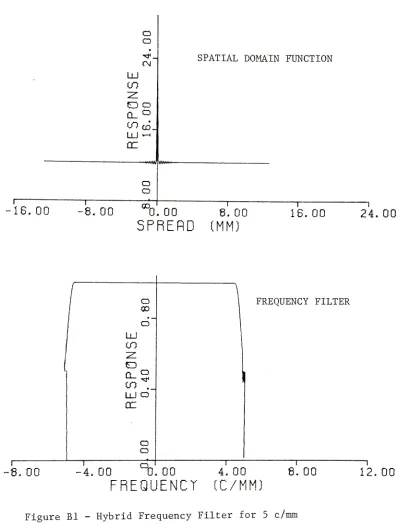
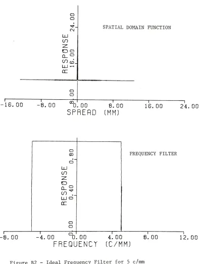
Figure Bl - _Hybrid

Frequency

Filter for 5 c/mm and

Spatial Domain Function, ,.,,,,,,.,,,,.,,,.,,,,,,,,,,,,,.,37

Figure B2

-Ideal

Frequency

Filter for 5 c/mm and

Spatial Domain Function. ..,...,.,,..,.,.,,..,,,...,..,38

Figure B3 - _Hybrid

Frequency

Filter for 4 c/mm and

Spatial Domain Function.,..,,,.,,..,,, ,,.,,,,,,.,...

39-Figure B.4 - Ideal

Frequency

Filter for 4 c/mm and

Spatial Domain Function. ,,.,,,,.,,..,,,,..,,,,,,,.,,,,.,,4Q

Figure B5

-Hybrid

Frequency

Filter for 3 c/mm and

Spatial Domain Function..,,..,.,..,.,....,,,,.,.,,..,,,..41

Figure B6 - _Ideal

Frequency

Filter for 3 c/mm and

Spatial Domain Function 42

Figure B7 - _Hybrid

Frequency

Filter for 2 c/mm and

Spatial Domain Function 43

Figure R8 - Ideal

Frequency

Filter for 2 c/mm and

Figure B1Q - _Ideal

Frequency

Filter

for

1 c/mm and

Spatial Domain Function, , . , . , 46

Figure CI

-Original Data (No

frequency filtering

or

edge tapering).. .,,...,..., ,.,,,., ,.,,,,.,48

Figure C2 - _Data

with 5 c/mm

Frequency

Filtering., , , 49

Figure C3

-Data with 3 c/mm

Frequency

Filtering, ..,.,.,.,,,,,...,,,.50

Figure C4 - _Data

with 1 c/mm

Frequency

Filtering...,,...,., , .

, . ,51

Figure Dl

-Original Data , .,,.,,..,.,....,.,.... 53

Figure D2

-Data with 5 c/mm

Frequency

Filter Applied, .,...,.,.,.,.. .54

Figure D3

-Data with 4 c/mm

Frequency

Filter _Applied,. , . ,55

Figure D4 - _Data

with 3 c/mm

Frequency

Filter

Applied,

,,.,.. ,56

Figure D5 Data with 2 c/mm

Frequency

Filter Applied..,.,,,.,,,...,, .57

Figure D6

-Data with 1 c/mm

Frequency

Filter Applied. ,...,.,,.,,,,, .58

Figure D7 - _{Original Data} (High. _{Contrast Imagel,}

....,..,....,, 59 Figure. D8 Data with 5 c/mm

Frequency

Filter Applied

(High. Contrast

Imagel,

.,,.,,,,,,,,..,.,.,,,.,,..,,.,.,,,,,6Q

Figure D9 - _Data

with 4 c/mm

Frequency

Filter Applied

(high.

Contrast

Image)

.,,.,,,*, ,,.,....,.,,,..,.,,,.. , ...61

Figure Did Data with 3 c/mm

Frequency

Filter Applied

(High Contrast Imagel- ,,,,,,,.,,, .62

Figure Dll

-Data with. 2 c/mm

Frequency

Filter Applied

(High Contrast Imagel, ..,,,.,,,.,.,... , . . . , 63

Figure D12

-Data with 1 c/mm

Frequency

Filter Applied

(High. Contrast Imagel.. ,....,,,,,.,.,...,,,.., . 64

[image:8.539.57.490.88.678.2]

The human eye, it's optics and _{photoreceptors,} and the nervous

system which transmits signals to the visual _cortex, are the main _comp

onents of the human visual system. The complete function of this system

are not

fully

understood due to the complex functions of the brain in

it's interpretations of visual signals.

However,

the consideration that

the eye behaves as a linear system have led to the application of linear

systems _analysis, Fourier _analysis, and signal _processing

theory

to

vision science. The modulation transfer function

(MTF)

is a measure of

how

frequency

information will be degraded as it passes through a system.

Since this is a sine_{wave response}

characteristic, many experimenters

have classified thevisual modulation transfer function

by

_measuring the

7

2

3

4

5

eye's response to purely sinusiodal information. ' ' ' '

Since the

eye's optical system changes with object/scene _{luminance changes,} the

visual MTF

(VTF)

must be a function of these changes. As the scene

6

luminance _changes, the pupil diameter of the eye changes. Shade relates

field luminance and pupil diameter. Table 1 tabulates some of these

values. Figure 1 shows the variation of the visual MTF as the pupil size

changes. There is some question as to the exact shape of the visual MTF

at _{very low frequencies} (less than one cycle per millimeter) but this

experiment is not working in the region so the information in Figure 1

can be assumed to be valid for the region of study.

relat-it is hoped to demonstrate the _{relationship between} the VTF and the

frequency

content of the image. It is felt that complex images are a

more valid criterion for the basis of VTF functions rather than simple

sinusoidal images. This information is deemed valuable when images are

7

digitally

processed in the context of the visual system.

Table 1

Scene Luminance and

Resulting

Pupil Size

Scene Luminance Pupil Diameter

(in

foot-lamberts)

(.in mm)

4 x

-4

6.5

4 x

-3

5.9

0.04 5.3

0.4 4.7

1.0 4.4

4.0 3.9

10 3.6

40 3.0

100 2.8

400

1000

2.3

1.00 80 u 01 m w a cfl U H C O H 3 13 O QJ en C o en a) Pi 0) .60 -,40 -,20 + -2.0 mm -Performance of Ideal System

40 80 120 160

Spatial

Frequency

(c/mm

-on retina)

200

Figure 1 - _{Modulation Transfer}

Function

theory

9

be given here but a more complete discussion can be found in

Papoulis,

Bracewell,

and

Brigham,

_among others.

The Fourier transform is _generally be stated to be:

F(l/)=

/f(x)

_{exp(-/27Txu) dx.}

This transform also exhibits the properties of _{reversibility} such that

a function defined in the

frequency

domain can also be defined in the

spatial domain by:

f(x)=

I

F(V)

expC+i27Txu) dv.

Becuase an image is defined in two spatial

dimensions,

the Fourier

transform pair can also be defined in two dimensions:

F(tt,

V)=J_J

f(x>y)

exp(-/27rCux + v/y)) dx

dy

f

(x,y)=/

r~F(u,v/)

exp(+/2tf-(ux + _Vy)) du. du.

Very

often, complex signals cannot be _readily defined as

continuous functions but are taken to be a sequence of discrete points.

The discrete Fourier transform

(DFT)

pair is the transform of a sequence

of N samples taken ax units apart. In one

dimension,

the discrete

Fourier transform pair is:

N-l

F(V)=^X1

f(x)

exp(-/2-Vx/N) x=0

N-l

f(x)=

^

Yl

F(U)

exp(+/2?n;x/N)

F(u,l>)= -~

S

2

f(x,y)

expC-i'2^Cax/M + Uy/N)

)

x=0 y=0

M-l N-l

fCx,y)=

m^ a^

^

F(a,u)

exp(+/2^(ax/M

+ _Vy/N))

F((X,U)

or

F(U)

, are often The modulus of these

functions,

called the Fourier spectra of the images or signals. These spectra show

the amplitude of the various sine-cosine pairs at the frequencies

contained in the signals.

When the Fourier transform is used to related the spatial-space

and the

frequency

domain,

one must always consider the effects that

operations in one domain will have on the other domain. As an example,

multiplication operations in one domain are convolution operations in

the other domain. These interrelated effects must be taken into consid

eration when

designing

filters to be used in one domain. Considerations

for the filters designed in this experiment are descussed in the

EXPERIMENTAL section and in APPENDIX B.

When a signal is sampled over finite

limits,

it is said to be

truncated at those limits. This is because there is no information

about the signal outside of those limits. The act of _sampling a signal

in one domainn causes the transform of that signal in the other domain to

become an

infinitely

periodic function. This means that the discrete

Fourier transform gives the results for a truncated original signal as

though this signal were

infinitely

periodic, with one period

being

the

in the

frequency

domain. This error introduced into the- transform is

called

"wraparound".

In order to

keep

this effect to a minimum, it is

U

necessary to taper the original function down to zero at the edges.

This causes some loss of information at the edges of the function but

eliminates the false

frequency

characteristics caused

by

the wraparound

The test image used for the experiment is an Indoor scene.

The

digitized

data for this scene was supplied

by

the thesis advisor.

The image is one of a set that has wide use in

industry

for image exper

imentation. This scene was selected because it contains adequate detail

for this experiment. The test image is represented

by

a two-dimensional

array, 256 x

256,

with each point

having

a brightness value between 1 and

256. Figure 2 is a representation of the test image.

A Fast Fourier transform was used to compute the

frequency

spectrum of the test image. The image is composed of an _array of 64,000

words of data. To allow this to be processed _using a two-dimensional

Fast Fourier transform

(FFT)

, all of the image data would have to be

resident in the _working core of the host computer. In this _experiment,

all FFT calculations were done on the RIT Honeywell-Xerox Sigma 9

computer system.

However,

the maximum allowable core use for one user at

one time is 32,000 words. This necessitated the design of an FFT program

which processed less than the full picture at one time. It is _generally

assumed that the information in one dimension of the image can be

oper-13

ated upon _seperatly from information in the other

dimension,

so it can

be shown that the two-dimensional discrete transform discussed in the

introduction can be applied one dimension at a time.

Using

this as a

basic premise, a program was written that applies a one-dimensional FFT

[image:16.539.84.407.127.438.2]

edges of the image to zero. The filter consisted of a raised cosine

function that goes from a value of one to a value of zero in 25 points

U

along each edge.

The actual FFT routine used in this experiment is a FORTRAN

subroutine called

FOURG,

which was developed

by

Mr. Norman Brenner of

14

the MIT Lincoln Laboratory. This routine is _generally available in the

industry

today. It was developed to accept _any number of data points, N

rather than 2 points as in most FFT routines. Although the experiment

Q

only uses 256

(2

)

points in the FFT at a _time, this subroutine was used so that the number of data points processed could _{be completely}

flexible.

The program written for this experiment that applies the

tapering

filter and takes the _minus-J transform of the orignal image data is

called MINTRANS. It is listed in APPENDIX _{A along} with other programs

written for this experiment. This program executed in _{approximately}

9 minutes of computation

(CPU)

time on the RIT Sigma.

The filters used in the

frequency

domain in this experiment

were designed with two major considerations. The first was that

they

should be as _{sharp cutting} as possible. This suggested a rectangle

function should be used.

However,

the other consideration was the effect

of the filter in the spatial space after the image was reconstructed.

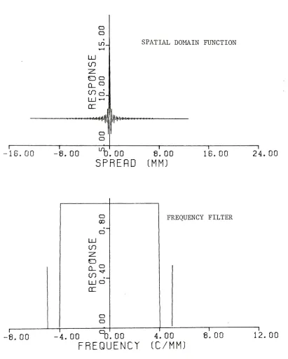
Since the Fourier transform of the rectangle function is the sine

Figure 3 shows an ideal rectangle filter which cuts at 2 cycles per

millimeter

(c/mm)

in the

frequency

_domain and the _resulting sine function

in the spatial domain. In this _case, the spread of the sine function is

over 16 millimeters

(mm)

in the reconstructed image. The visual effect

in the reconstructed image due to the ripples in the sine function is

known as

"ringing".

A filter should be developed that keeps ringing to

a minimum.

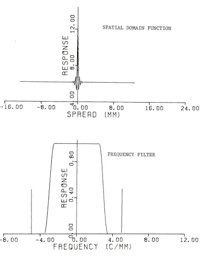
A hybrid

frequency filter,

_combining the characteristics of both

the rectangle filter and a raised cosine

function,

was used in this

experiment. One half of the cosine cycle was scaled to modulate from

100% to 0% in 25 points of the array. Figure 4 shows a hybrid

frequency

filter which is at 50% at 2 c/mm. The 50% point of the filters used

in this experiment was defined to be the cutoff

frequency

of the filter.

The resultant function in the spatial domain is also shown in Figure 4.

The hybrid filter _greatly reduces the spread in the spatial domain

caused

by

the convolution of the filter's transform with the image points.

Using

the program MINTRANS as a

basis,

a program was developed as

a _plus-J transform to back-transform the filtered

frequency

domain data.

This program also applied the

frequency

filters that were developed. It

is listed in APPENDIX A as the program PLUSTRANS.

The sampled

frequency

domain of a signal is related to its

J5

spatial space

by

the Nyquist Equation:

NAfAX=1,

where N is the number of samples, Af is the

frequency

interval,

and ax

o o LU en -z. o

-en . LUOO DC -^-^n^aa/vVVAAAA/1 o o -16.00 -8.00

Spatial Domain Function

0.00

SPRERD

8.00

(MM)

16.00

24.00

o 00

Frequency

Filter Function

LU en -z. d tn ._ LU O QC

1 1 1 i i

-8.00 4.00

^.00

4.00

FREQUENCY

(C/MM)

8.00

12.00

Figure 3

-Rectangle

Frequency

Filter [image:19.539.52.473.37.595.2]

o o

LU cn

o

^

in.

LUCO CC

o

-16.00 -8.00

Spatial Domain Function

^|^~

0.00

SPREAD

8.00

(MM)

16.00

24.00

-8.00

Hybrid

Frequency

Filter

4.

00

~0.

00

4.

00

FREQUENCY

(C/MM)

8.00

12.00

Figure 4 - _Hybrid

Frequency

Filter [image:20.539.55.459.57.649.2]

signal given by:

max 2ax

In this _{experiment, only} 256 samples are available _along one dimension.

Once the size of the final image is

defined,

it's maximum

frequency

and

frequency

sampling interval are defined. The published data on visual MTF

given in the INTRODUCTION shows that the area of the

frequency

response

under test is from one to ten cycles per millimeter on the image. This

criterion will define the visual angle _necessary to be subtended

by

the

prints to give the

frequency

range required.

The

frequency

filters used in this experiment were designed to

cut off at frequencies of 1 c/mm, 2 c/mm, 3 c/mm, 4 c/mm and 5 c/mm on

the prints. APPENDIX B shows these filters along with their respective

spatial domain pairs. Also in this appendix are the equivelant "ideal"

rectangle filters and their spatial domain pairs for comparison.

An output scheme was developed for this experiment when no

suitable established routine could be located through local

industry

that was accessable to the author. Because of the limited number of

alternative methods, an output routine was written for a Tektronix 4014

Graphisc CRT terminal (with the Extended Graphics

Option),

and a Tektronix

4631 Hard

Copy

Unit,

which was available through the thesis advisor.

The output method uses a scheme of

halftoning

to produce the

desired desities.

However,

due to the terminals screen _resolution,

each halftone pixel was capable of produceing only sixty-four levels of

be turned on or off. The size of the points _{making up} each pixel is the

smallest available on the terminal. The pixels are created from the

center of the _array outward such that the pixel appears to be a _growing

dot as the

density

value at the point increases. Since the output scheme

outputs _only sixty-four levels while 256 levels are

input,

the program

also rescales the data.

Many

of the factors in an output system of this type have not been

throughly

investigated since the purpose of this experiment has

not been to design an output system. The effects of _{beam size,} screen

noise, and the reproduction characteristics of the hard copy unit have

not been studied here. All of these factors were

initially

adjusted to

give a print acceptable for the experiment and then held constant

throughout the remainder of the output process.

The FORTRAN program OUTPUT is listed in APPENDIX A. This is the

program used to produce the images used in this experiment. The

output-ing

was done using the terminal equipment described above and a Data General ECLIPSE S230 minicomputer. Images were output at a rate of

about one image _every two and a half hours of user time. This mini

computer was used because the system had certain intrinsic characteristics

that allowed faster output than either the RIT Sigma system or the Xerox

Sigma system. These characteristics allowed for a more efficient program

and a higher avaialble output baud rate.

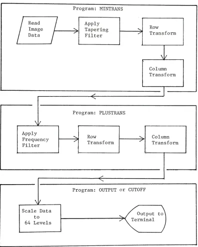
Figure 5 is an overall block diagram

describing

the data

processing and output scheme used in this experiment. It shows the

Read Image Data

^L

Apply

Frequency

Filter

it

Scale Data to 64 Levels Program: MINTRANS ">

Apply

Tapering

Filter "> Row Transform

Ak

Column Transform < Program: PLUSTRANS "> Row Transform "> Column Transform <

Program: OUTPUT or CUTOFF

Output to'

"/\

Terminal

Figure 5 - Block Diagram _of Data

[image:23.539.61.458.107.602.2]

Another method of _outputing the data to the Tektronix terminal

was a threshold level program called CUTOFF. This program prints a

completely black pixel of the brightness level of the data was below

a selected value. If the data was above that

level,

the area was left

blank

(white).

This produced a set of test images of high contrast.

The _resulting images from the hard _copy unit used in this experiment

contained a ripple effect _along the x-direction. This effect was constant

in all of the test images.

The two sets of images produced from the data were set _up such

that the illumination level and _viewing angle would allow for

comparison of the results of this experiment with the earlier experiments

presented in the introduction. The illumination level was set to 72

foot-lamberts. The images were placed such that

they

subtended a visual

angle of 3.8 to the observer. Under these _conditions, the images were

viewed two at a time for pair comparison analysis. The results of this

pair comparison has been evaluated _using the

"Rickmers-Todd

Method For

16

Analysis of Subjective Judgements1.1

The observers were asked to rate

the images

by

sharpness for both sets of data. The observers were

asked to discount the ripple effect in the high contrast set of images

and attempt to judge sharpness of the images with the various _gray levels

RESULTS OF EXPERIMENT

The two sets of images are shown in APPENDIX D. The tabular results

of the pair comparisons are shown in APPENDIX E. The Rickmers - _Todd

method places the images on a scale _ranking their relative

position.*

Figures 6 and 7 show the _resulting ranks of the two sets of images.

Both figures show the average of the results of the observers that were judged to be consistant and the average of the results of all of the

observers. For both sets of

images,

the consistant observers were found

to _{significantly} agree in their evaluation

(using

0.05 level of

significance). For the prints with _varying levels of gray, the

coefficient of concordance for the consistant observers was 0,95.

The coefficient of concordance for the consistant observers of the

high contrast prints was 0.9.1,

This scale is not a true interval scale but Interpretations as to the

relative similarity or difference of prints can be made

by

noting the

by

2&4 3 l

1

,

,

1

4 2 3 6 5

Ranks

by

All Observers

Figure 6 - _Rank

Ordering

of Images with

Varying

Levels

2 3 4&5

1

1

h

2 3 4 5

Ranks

by

All Observers

Figure 7 - _Rank

INTERPRETATION OF RESULTS

The results shown in Figures 6 and 7 are in overall agreement

with, earlier experimental results, J'/->i>^'-}

The image with _{varying levels} of _gray that had a

frequency

cutoff

of 4 c/mm Is ranked equal with the image have 2 c/mm cutoff. This is

felt to be due to the fact that the 4 c/mm image had a slightly

higher overall brightness in comparison with the rest of the prints.

The reason for this is perhaps some

inconsistancy

in the hard _copy unit

of the Tektronix terminal at the time of output. Since sharpness (or

J7

acutance) is related to

density

differences,

differences in the overall

density

levels of the images are contributing factors in the subjective

evaluation of sharpness. When the high contast images of the same data

were _ranked, all of the images were ranked in the order predicted

by

previous experiments.

The reversal of the order of the images with 5 c/mm cutoff and

6 c/mm cutoff in the ranking of the images with _varying levels of _gray

might also be attributed to the above effect. Since theory predicts

that the eye's

frequency

response to these images _{is approximately} the

same, the _proximity of these two images in the _{ranking indicates very}

little difference judged between these images. In the case of the high

contrast

images,

all of the upper

frequency

cutoffs are grouped together.

This shows a _similarity in there judgement as predicted

by

theory.

this _type, certain changes might be made in the experiment.

First,

a

better,

more consistant output system needs to be used. A more through

understanding of the effects of the variables of the output system are

necessary. Controls on the output system to produce prints which _vary

only in their sharpness due to the

frequency

cutoff of the data is also

necessary.

Secondly,

enough data must be used such, that higher frequencies

outside of the visual MTF range are available. This will allow for more

through

testing

of the visual effects of

frequency

manipulation

CONCLUSIONS

D

The modulation transfer function of the human visual system

developed through simple sine-wave targets has been demonstrated to

work for complex images.

2)

The effect of image contrast has been shown to be. signaficant on

BIBLIOGRAPHY

McCann,

J.J.,

R.L.

Savoy,

and J. A.

Hall,

Jr.

"Visibility

of Low

Frequency

Sine-Wave Targets: Dependence on the Number of Cycles

and Surround

Parameters",

Vision

Research,

1978,

18.

2

Watanabe,

A.,

T.

Mori,

S.

Nagata,

and K. Hiwatashi.

"Spatial

Sine-Wave

Response of the Human Visual

System",

Vision

Research,

1968,

18.

3

Carlson,

C.R.,

R.W.

Cohen,

and I. Gorog.

"Visual

Processing

of Simple

Two-Dimensional Sine-Wave Luminance

Gratings",

Vision

Research,

1977,

17.

4

Wilson,

H,R. and S.C. Giese.

"Threshold

Visibility

of

Frequency

Gradient

Patterns",

Vision

Research,

1977,

17.

Campbell,

F.W. and J.G. Robson.

"Application

of Fourier Analysis to the

Visibility

of

Gratings",

J.

Physiol.,

1968,

197.

6

Shade,

O.H.

"Optical

and Photoelectric

Anolog

of the

Eye",

J. Opt. Soc.

Am. ,

1956,

46.

7

Stockham, T.G.,

Jr.

"Image

Processing

in the Context of a Visual

Model",

Proceedings of the

IEEE,

July 1972,

60(7).

g

Campbell,

F.W, and R.W.

Gubisch,

"Optical

Quality

of the Human

Eye",

J.

Physiol.,

1966, 186,

pg. 570,

9

Papoulis,

A. The Fourier Integral and Its Applications. New York:

McGraw

-Hill,

1962.

Bracewell,

R.N. The Fourier Transform and Its

Applications,

2nd ed..

New York: McGraw

-Hill,

1978.

Brigham,

E.O. The Fast Fourier Transform. Englewood

Cliffs,

NJ;

Prentice

-Hall,

1974.

13

Gonzalez,

R.C. and P. Wintz. Digital Image Processing.

Reading,

Mass.: Addison

-Wesley,

1977,

pg. 50-52.

14

Brenner,

N. Various Program Listings and

Descriptions,

Supplied

by

Thesis Advisor.

Gonzalez and Wintz. Digital Image Processing, pg. 70-75.

16

Rickmers,

A.

"Rickmers

-Todd Method For Analysis of Subjective

Judgements",

Handout from Author.

11

James, T.H.,

ed. The

Theory

of the Photographic

Process,

4th ed. . New York:

Macmillian,

1977,

pg. 602-603.

1 S

Hamming,

R.W. Digital Filters. Englewood

Cliffs,

NJ: Prentice

-Hall,

1977,

pg. 178-179.

19

General References

Andrews,

H.C. and B.R. Hunt. Digital Image Restoration. Englewood

Cliffs,

NJ: Prentice

-Hall,

1977.

Bracewll,

R.N. The Fourier Transform and Its

Applications,

2nd ed..

New York:

McGraw-Hill,

1978.

Brigham,

E.O. The Fast Fourier Transform. Englewood

Cliffs,

NJ: Prentice

-Hall,

1974.

Chavez,

Noel.

"The

Modification of Simple Images

by

Fourier Transform Manipulation". RIT Bachelor of Science

Thesis,

June 1979.

Cooley,

J.W. and J.W.

Tukey,

"An

Algorithm for the Machine Calculation of

Complex Fourier

Series",

Math.

Computation,

April

1965,

19.

Gaskill,

J.D. Linear

Systems,

Fourier

Transforms,

and Optics. New York: John

Wiley,

1978.

" ' "

Gonzalez,

R.C. and P. Wintz. Digital Image Processing.

Reading,

Mass.: Addison

-Wesley,

1977.

Pratt,

W.K. Digital Image Processing. New York: John

Wiley,

1978.

APPENDIX A

Computer Programs Developed

for this Experiment

This appendix contains computer programs that where written for

this experiment

by

the author. The programs MINTRANS and PLUSTRANS are

written to use XEROX EXTENDED FORTRAN IV but should be compatable with

most other FORTRAN compilers. The program OUTPUT was written _using the

Data General FORTRAN V compiler, as was the program CUTOFF.

Both MINTRANS and PLUSTRANS use the subroutine FOURG. This sub

routine is the Fast Fourier Transform used in this project. Other

FFT routines could be substituted for FOURG. FOURG is not listed in this

appendix because it is generally available and other FFT routines can be

CCC FILENAME: MINTRANS

CCC THIS PROGRAM TAKES THE MINUS I TRANSFORM OF A 256 X 256 ARRAY

CCC USING A SERIES OF ONE-DIMENSIONAL FFT'S TO REDUCE WORKING CORE

CCC MEMORY SPACE.

CCC

C DIMENSION ARRAYS

C

REAL

INREAL(256)

,INIMAG(256),OUTREAL(256),

*OUTIMAG(256)

,TRANSFORM(2,256) ,WORK(256),

*FILTER(256)

INTEGER IN!

(256)

C

C CREAT TAPERING FILTER

C

DATA FILTER/256*

1.0/

FACTOR = _{3.141593/26.0}

DO 50 1=1,26

FILTER(27-I)=(COS(FLOAT (I)*FACTOR)+1.0)/2.0

50 FILTER(240+I)=(COS (FLOAT(I)*FACTOR)+1.0)/2.0

C

C READ IN AND TRANSFORM ROW DATA AND OUTPUT TO A TEMPORARY FILE

C

DO 300 1=1,256

CALL BUFFIN(1,1,IN1,256)

DO 100 J=l,256

TRANSFORM(l,J)=FLOAT(INl(J))*FILTER(I)*FILTER(J)

100 TRANSFORM

(2,

J)

=0,0

CALL FOURG(TRANSFORM,

256,-1, WORK)

DO 200 K=l,256

OUTREAL

(K)

=TRANSFORM

(

1_,

K)

200 OUTIMAG(K)=TRANSFORM(2,K)

CALL BUFFOUT

(2,1,

OUTREAL,

256)

300 CALL BUFFOUT(3,l,OUTIMAG,256)

REWIND 2

REWIND 3

C

C READ IN DATA FROM TRANSFORM TEPORARY FILES AND TRANSFORM COLUMNS AND

C OUTPUT TO FILES FOR DISC STORAGE

C

DO 600 M=l,256

DO 400 N=l,256

CALL BUFFIN(2,1,INREAL,M)

CALL BUFFIN

(3,1,

INIMAG,M)

TRANSFORM( 1,N)=INREAL

(M)

400 TRANSFORMS,N)=INIMAG(M)

CALL FOURG

(TRANSFORM, 256,-1, WORK)

DO 500 1=1,256

OUTREAL

(I)

=TRANSFORM(1,

I)

CCC FILENAME:MINTRANS

(CONTINUED)

C

CALL

BUFFOUT(4,l,OUTREAL,256)

CALL

BUFFOUT(5,l,OUTIMAG,256)

REWIND 2

600 REWIND 3 STOP

CCC FILENAME: PLUSTRANS

CCC THIS PROGRAM TAKES THE PLUS I TRANSFORM OF A 256 X 256 ARRAY USING

CCC A SERIES OF ONE-DIMENSIOAL FFT'S TO REDUCE WORKING CORE MEMORY

CCC SPACE.

CCC THIS PROGRAM ALSO APPLIES THE SELECTED FREQUENCY FILTER TO THE INPUT

CCC DATA.

CCC

C DIMENSION AND INITIALIZE ARRAYS

C

REAL

INREAL(256)

,INIMAG(256) ,OUTREAL(256),OUTIMAG(256),

*TRANSFORM(2,256),WORK(2,256),INl(256),IN2C256),FILTER(256)

INTEGER

IOUTREAL(256)

DATA FILTER/256*0.0/

FACTOR=3.141593/26.0

C

C SELECT FILTER TO BE USED ON INPUT DATA

C

READ

100,

IFIL

100 FORMAT

(II)

IF(IFIL.EQ.5)

GOTO 10

IF(IFIL.EQ.

4)

GOTO 20

IF(IFIL.EQ.

3)

GOTO 30

IF(IFIL.EQ.

2)

GOTO 40

IF(IFIL.EQ.l)

GOTO 50

C

C CREAT THE NECESSARY FILTER C

10 DO 1100 1=1,14

FILTER(I+115)=(.COS(FLOAT(I)*FACTOR)+1.0)/2.0

1100 FILTER(141-I)=(COS(FLOAT(I)*FACTOR)+1.0)/2.0

GOTO 200

20 DO 1150 1=1,70

1150 FILTER(1+9

3)

=0.0

DO 1200 1=1,26

FILTER(I+89)=(COS(FLOAT(I)*FACTOR)+1.0)/2.0

1200 FILTER(167-I)=(COS(FLOAT(I)*FACTOR)+1.0)/2.0

GOTO 200

30 DO 1250 1=1,129

1250 FILTER(I+63)=0.0

DO 1300 1=1,26

FILTER(I+63)=(COS(FLOAT(I)*FACTOR)+1.0)/2.0

1300 FILTER(193-I)=(COS(FLOAT(I)*FACTOR)+1.0)/2.0 GOTO 200

40 DO 1350 1=1,179

1350 FILTER

(1+38)

=0.0 DO 1400 1=1,26

FILTER(I+38)=(COS(FLOAT(I)*FACTOR)+1.0)/2.0

1400 FILTER(218-I)=(COS(FLOAT(I)*FACTOR)+1.0)/2.0

GOTO 200

CCC FILENAME: PLUSTRANS

(

CONTINUED

)

C

DO _{1500 1=1,26}

FILTER

(1+1

3)=

(COS (FLOAT

(I)

*FACTOR)+l

.

0) /2

.0

1500 FILTER(243-1)=

(COS (FLOAT

(I)

*FACTOR)+1.0)/2.0

C

C READ

IN, FILTER,

AND TRANSFORM ROW DATA

C

200 DO 300 1=1,256

CALL

BUFFIN(1,1,IN1,256)

CALL

BUFFIN(10,1,IN1,256)

DO _{110 J=l,256}

TRANSFORMQ

,

J)

=IN1

(

J)

*FILTER(I)

*FILTER(

J)

110

TRANSFORMS,

J)=IN2

(J) *FILTER(I)*FILTER(J)

CALL FOURG

(TRANSFORM,

256,

+1,

WORK)

C

C SCALE DATA AND OUTPUT TO TEMPORARY FILES

C

DO 210 K=l,256

OUTREAL

(K)=TRANSFORM(l,K)/256.

210 OUTIMAG(K)=TRANSFORM(2,K)/256,

CALL BUFFOUT

(2,1,

OUTREAL,256)

300 CALL

BUFFOUT(3,l,OUTIMAG,256)

REWIND 2

REWIND 3

C

C READ IN DATA FROM TEMPORARY FILES AND TRANSFORM COLUMNS

C

DO 600 M=_1,256

DO 400 N=l,256

CALL BUFFIN

(2,1,

INREAL,

M)

CALL BUFFIN

(3,1,

INIMAG,

M)

TRANSFORM

(1,N)=INREAL(M)

400 TRANSFORM

(2,N)=INIMAG(M)

CALL FOURG

(TRANSFORM,

256,

+1, WORK)

C

C SCALE AND OUTPUT DATA TO DISC STORAGE

C

DO 500 1=1,256

The

following

_program,

PACK1,

is used to pack the data produced

by

PLUSTRANS such that there are 4 data values per word of _memory

(32 bits)

on the Sigma 9. This is equivalent to _packing one value per byte

(8 bits)

rather than per word. This facilitates data storage

by

_cutting required

space

by

a factor of four and allows ease of data transfer between the

Sigma 9 and the Eclipse S230 used to output the images. The program

OUTPUT unpacks the data for use.

CCC FILENAME: PACK1

CCC THIS FILE PACKS DATA TO FOUR VALUES PER WORD

(

ONE VALUE PER

CCC BYTE

)

USING A FORTRAN CONTROL PROGRAM AND A META-SYMBOL

CCC PACKING SUBROUTINE.

CCC

C CONTROL PROGRAM - READS IN DATA AT ONE VALUE PER

WORD,

CALLS C PACKING

SUBROUTINE,

AND OUTPUTS PACKED DATA.

C

INTEGER

IN1(256), 0UT1(64)

DO 200 1=1,256

CALL

BUFFIN(1,1,IN1,256)

IF(ICHECK(1).EQ.3)

GOTO 300

CALL

PACK(IN1,0UT1,64)

200 CALL

BUFFOUT(2,l,OUTl,64)

300 STOP

END

C

C META-SYMBOL PACKING SUBROUTINE C

SUBROUTINE PACK(IN,OUT,IWORDS)

IMPLICIT INTEGER

(A-Z)

BYTES=4*IW0RDS-1

S

LI,

4 0

S10 LW,9 *IN,4

S

AND,

9 =X'FF' S

STB,

9 *0UT,4

S AI,4 1

S CW,4 BYTES

S BLE 10S

CCC FILENAME: OUTPUT

CCC THIS PROGRAM READS IN THE PACKED IMAGE DATA AND PRODUCES A HALFTONE

CCC IMAGE ON A TEKTRONIX 4014 GRAPHICS TERMINAL FOR COPYING TO A HARD CCC COPY UNIT. THIS PROGRAM RUNS ON A DATA GENERAL ECLIPSE S230

CCC MINICOMPUTER UNDER THE FORTRAN V COMPILER.

CCC

C INITIALIZE ARRAYS

C

IMPLICIT INTEGER

(A-Z)

INTEGER

IN1(256),IN2(128),FNAME(16)

C

C OPEN DATA FILE OF

INTEREST,

INITIALIZE SCREEN POSITION C

READ(11,2)FNAME

2 FORMAT

(16S2)

DO 10 1=2,32

10

IF(BYTE(FNAME,I).EQ.040K)

BYTE(FNAME,I)=0 OPEN 3,FNAME,LEN=256

LODEN=l

TYPE ' FOR NEGATIVE ON

SCREEN,

TYPE "-"' READ

(11,

50)

INEG

TYPE ' INPUT UPPER CORNER COORDNINATES (X THEN

Y)

'

READ

(11,

30)

IIX

READ(11,30)

IY

30 FORMAT

(14)

50 FORMAT

(Al)

C

C INITIALIZE TERMINAL

MODE,

DRAW BORDER AROUND IMAGE

AREA,

SET C BEAM SPOT SIZE TO MINIMUM

C

CALL

INITT(O)

CALL TERM(3,4096)

CALL NEWPAG

CALL BORDER

(IIX,

IY)

CALL

TOUTPT(27)

CALL

TOUTPT(28)

CALL

TOUTPT(64)

C

C READ IN AND UNPACK DATA

C

DO 400 J=l,256

READ(3,100,END=999)(IN2(K),K=1.128)

100 FORMAT

(128A2)

K=l

DO 200 L=l,256 IN1(L)=BYTE(IN2,K)

K=K+1

C SCALE DATA TO 64 LEVELS AND CALL PIXEL ROUTINE TO PRODUCE

C HALFTONE PATTERN

C

IX=IIX

DO 300 1=1,256

IF(INEG.EQ.2H-)IN1(I)=110-IN1(I)

IF(IN1(I).LT,0)

IN1(I)=0

DEN=IFIX(FLOAT(IN1(I))/4.0)

IF

(DEN.

GT,

64)

DEN=64

CALL

PIXEL(IX,IY,DEN,LODEN)

300 IX=IX+8

400 IY=IY-8

C

C MAKE A HARD COPY OF THE FINISHED IMAGE AND END C

CALL HDCOPY CALL

FINTT(0,0)

GOTO 500

999 TYPE

'END

OF FILE

-ERROR ON READ'

500 STOP

END C

C PIXEL SUBROUTINE - _ROUTINE

WHICH PRODUCES HALFTONE "DOTS" C

SUBROUTINE PIXEL

(IX,

IY_,DEN,

LODEN)

IMPLICIT INTEGER

(A-Z)

INTEGER

XMOV(64),YMOV(64)

DATA XMOV?

*0, 1,-1, 1,-1, 1,-2, 1,-2, 3,

-2,

1,-2, 3,

-3,

3, 0,-3, 1,1, 2,

5,

*3,

-1,3,-5,

5,

-5,

4,

-3,

0,3, 1,-5, 6,

-7,

3, 1,0,

-1,4,-7,

*6,

-5,

5,

-5,

4,

-3,

5,

-7,

7,

-7,

2, 3,

-5,

7,

-6,

5,

-5,

5,

1,-7, 0,7,

0,-7/

*YMOV/

*0,

1,0,

-1,2,-3,

1,1,

-2,

3,

-1,-1,

2,

-3,

3,

-3,

4,

-5,

3,-1,

*3,

-5,

2, 1,-2, 3, 1,-5, 5,

-5,

4,

-3,

2,

-1,4,-7,

7,

-7,

3,1,

*2,

-5,

0,5,

-6,

7,

-2, -3,

0,3,

-5,

7,

-6,

5, 1,-7, 0,7,

-6,

5,

-6,

7,

-7,

7/

IF(DEN.EQ.

LODEN)

RETURN

CALL

MOVABS(IX,IY)

DO 100 IVAL=1,DEN

CALL PNTREL

(XMOV(IVAL)

,YMOV

(IVAL)

)

100 CONTINUE RETURN END C

C BORDER SUBROUTINE - _DRAWS BORDER AROUND IMAGE AREA

C BORDER SUBROUTINE

(_

CONTINUED

)

C

CALL

DRWABSClX+2064,IY-2064)

CALL

DRWABS(IX,IY-2064)

CALL

DRWABS(IX,IY)

RETURN

CCC BELOW THIS THRESHOLD CAUSES A FULL BLACK PIXEL TO BE PRODUCED.

CCC ALL DATA ABOVE THE THRESHOLD IS NOT PRINTED.

CCC THIS PROGRAM RUNS ON A DATA GENERAL ECLIPSE S230

CCC MINICOMPUTER UNDER THE FORTRAN V COMPILER.

CCC

C INITIALIZE ARRAYS

C

IMPLICIT INTEGER

(A-Z)

INTEGER INI(2 5 6

)

,IN2

(

1 2 8

)

,FNAME

(1

6

)

C

C OPEN DATA FILE OF INTEREST

C

TYPE " DATA FILE NAME? "

READ

(11,

2)

FNAME

2 FORMAT

(16S2)

DO 10 1=2,32

10 IF(BYTE(FNAME,I),EQ.040K) BYTE

(FNAME,

I)

=0

OPEN 3,FNAME,LEN=256

C

C SET THRESHOLD LEVEL

C

55 TYPE " CUTOFF LEVEL?

(1-256),

"

READ(.11,60)IVAL

60 FORMAT

(13)

IFCIVAL.EQ.999) GO TO 500 C

C INITIALIZE TERMINAL

MODE,

THEN READ AND UNPACK DATA

C

CALL

INITT(O)

CALL NEWPAG

DO 400 1=518,263,-1

READ(.3,1,END=999) (IN2

(K)

,K=1 ,128)

1 FORMAT

(1

2

8A2)

DO 200 L=l,256

200 IN1(L)=BYTE(IN2,L)

C

C OUTPUT PIXELS WHEN DATA IS LESS THAN THRESHOLD

C

DO 400 K=384,639

IF(IN1(K-383).LT.IVAL) CALL PNTABSC2*K-5

12,

2*1-390)

400 CONTINUE

CALL FLNTT(0,0)

C

C LOOP BACK TO SET DIFFERENT THRESHOLD

C OR END

GO TO 55

999 TYPE

"END

OF FILE"

APPENDIX B

A Comparison of Hybrid

Frequency

Filters

and the Equivalent Ideal

(Rectangle)

Filter

This appendix contains figures _showing the hybrid

frequency

filters used in this experiment. These are shown _along one axis of the

two-dimensional filter _actually used. The spatial domain function assoc

iated with each filter is shown with the filter. On the

following

page,

the equivalent ideal

(rectangle)

filter and it's spatial domain function

are shown for comparison.

The two vertical lines on each of the

frequency

domain figures

are the limits of the

frequency

content in the image (from the Nyquist

o o

UJ in z

Oa

t-n&A

LU -< DC

-16.

00

-8.00

o

o

oa.

SPATIAL DOMAIN FUNCTION

0.00

SPREAD

8.00

(MM)

16.00

"24.00

FREQUENCY FILTER

-8.

00

-4

00

0.

00

FREQUENCY

4.00

(C/MM)

8.00

12.

00

Figure Bl - Hybrid

Frequency

Filter for 5 c/mm [image:45.539.58.456.81.605.2]

o o

"*_

CM

LU in z.

cnoj- LU-QZ

-16.00 -8.00

o o

co

SPATIAL DOMAIN FUNCTION

0.00

SPREAD

8.00

(MM)

16.00

24. 00

FREQUENCY FILTER

-8.00 4.

00

0. 00

FREQUENCY

4.00

(C/MM)

8.00

12.00

Figure B2 - Ideal

Frequency

Filter for 5 c/mm [image:46.539.60.456.80.601.2]

o o CM LU in z Oo 0_ CO CD LU-o o -16.00 -8.00 OCL

SPATIAL DOMAIN FUNCTION

0.00

SPREAD

8.00

(MM)

16.

00

24.00

o CO LU CO z o CO . LUO CC o o -8.00 Q_ FREQUENCY FILTER

4.

00

~0.

00

4.

00

FREQUENCY

(C/MM)

[image:47.539.60.456.81.597.2]

8.00

12.00

Figure B3 - Hybrid

Frequency

Filter for 4 c/mm

o

o

LOJ

LU CO

W*^Mi^M

-16.

00

-8.00

SPATIAL DOMAIN FUNCTION

^^V^ft^WwY-V^V-V^V-*.**

^.00

SPREAD

8.00

(MM)

16.00

24.00

FREQUENCY FILTER

-8.

00

-4

00

0.00

FREQUENCY

4.00

(C/MM)

8.

00

12.00

Figure B4 - _Ideal

Frequency

Filter for 4 c/mm [image:48.539.59.470.72.584.2]

o o CM_ LU CO z LUCO CC

16. 00

-8.

00

-l

o o

'*_

SPATIAL

_{DOMAIN FUNCTION}

0.00

SPREAD

8.00

(MM)

16.00

24.00

CO LU CO Z CO .. LUO CC o o FREQUENCY FILTER

-8.00 4.

00

^1).

00

4. 00

FREQUENCY

(C/MM)

8.00

12.00

Figure B5 - Hybrid

Frequency

Filter for 3 c/mm [image:49.539.55.459.82.588.2]

16.

00

o

o

CM_

LU CO z

in.

LUCO

CC

o

SPATIAL DOMAIN FUNCTION

~*n*>#*r**i\ffMm BJWVWlA'Vwvvuvv.^v-v.

-8.00

0.00

8.00

SPREAD

(MM)

16.00

24.00

-8.

00

-4

FREQUENCY FILTER

00

0.00

FREQUENCY

4.00

(C/MM)

8.00

12.00

Figure B6 - Ideal

Frequency

Filter for 3 c/mm [image:50.539.61.456.77.592.2]

-16.

00

o o

CM.

LU CO z

LUCO DC

~ir

o o

SPATIAL

_{DOMAIN FUNCTION}

-8.00

0.00

8.00

SPREAD

(MM)

16.00

24.00

-8.

00

FREQUENCY FILTER

-4.00

0.00

4.00

FREQUENCY

(C/MM)

[image:51.539.63.460.59.618.2]

8.00

12.00

Figure B7 - _Hybrid

o o

CMJ

LU CO z

o

0_a

a

CO .

LU00

CC

SPATIAL

_{DOMAIN FUNCTION}

^^wwvvVwl A/\/vwwvwv~

16.

00

-8.00

a o

^-0.00

SPREAD

8.00

(MM)

16.

00

~24.00

-8.

00

FREQUENCY FILTER

-4.00

0.00

4.00

FREQUENCY

(C/MM)

8.00

12.00

Figure B8 - Ideal

Frequency

Filter for 2 c/mm

CO

CC

SPATIAL DOMAIN FUNCTION

-16.00 -8.00

^.00

8.00

SPREAD

(MM)

16.00

24.00

-8.00

FREQUENCY FILTER

4.00

"0.00

4.00

FREQUENCY

(C/MM)

[image:53.539.55.456.60.648.2]

8.00

12.00

Figure B9 - Hybrid

Frequency

Filter for 1 c/mm

16.00

-8.00

o a

to

LU CO

SPATIAL DOMAIN FUNCTION

^.00

SPREAD

8.00

(MM)

16.00

24.00

LU CO

z

a o_ CO LU CC

a

FREQUENCY FILTER

-8.00 -4.00

CO

0.00

4.00

8.

00

12.00

FREQUENCY

(C/MM)

Figure B10 - _Ideal

Frequency

Filter for 1 c/mm [image:54.539.58.452.81.619.2]

APPENDIX C

A Comparison of One Data Record

for

Frequency

Filter Effects

This appendix shows the effects of

frequency filtering

on the

bri

ghtness values of one particular record. The record

(#128)

is taken from

the original data file and the files filtered at 5 c/mm, 3 c/mm, and

1 c/mm. The data record was picked arbitraraly,

This comparison shows the _smoothing effect of removing the high

300

1

350

-w

200

H H CO

1

150

100

-50

-ORIGINAL DATA

RECORD

t

128

1

-256 SCALING

50

150

ARRAY VALUE

250

Figure CI - _{Original Data} (No

frequency filtering

[image:56.539.53.482.62.525.2]

300

n

250

-200

>

H H

en

150

100

-50

-0

0

DATA UITH 5

C/NH

FILTERING

RECORD

*

128

1

-256 SCALING

100

50

150

ARRAY VALUE

200

300

250

Figure C2 - _{Data with} 5 _c/mm

300

i

250

-200

>

0

DATA UITH

3 C/flM

FILTERINlfc

RECORD

*

128

1

-256 SCALING

100

200

50

300

150

ARRAY VALUE

250

Figur C3 - _{Data with} 3 _c/mm

[image:58.539.52.484.79.499.2]

300

-250

-3

200

><

H H

CO

I

150

100

-50

-0

+

0

DATA UITH

1

C/MM FILTERING

RECORD

t

128

1

-256

SCALING

100

200

50

150

ARRAY VALUE

300

250

Figure C4 - Data _with. 1 _c/mm

[image:59.539.53.482.68.513.2]

APPENDIX D

Experimental Images

This appendix contains copies of the Images used in this experiment.

The first six images are those produced _using the program OUTPUT, The

last six images are those high contrast images produced

by

the program

[image:61.539.92.412.140.451.2]

[image:62.539.114.435.143.457.2]

[image:63.539.88.414.130.448.2]

Figure D3 - Data with.4 c/mm

Frequency

Filter

[image:64.539.86.411.134.451.2]

Figure D4 - Data _with 3 _c/mm

[image:65.539.112.435.135.456.2]

[image:66.539.87.411.135.448.2]

Figure D6 - _{Data with.}1 _c/mm

[image:67.539.85.402.134.448.2]

Figure D8 - Data with 5 c/mm Frequency Filter Applied

[image:68.539.85.401.130.436.2]

[image:69.539.119.442.126.439.2]

[image:70.539.87.413.135.447.2]

Figure DlQ - _{Data with.} 3 _c/mm

Frequency

Filter Applied

[image:71.539.82.408.135.445.2]

Figure Dll - _{Data with} 2 _c/mm

Frequency

Filter Applied

Figure D12 - Data with. 1 c/mm

Frequency

Filter Applied [image:72.539.89.411.128.448.2]

APPENDIX E

Tabular Results of Pair Comparisons

This appendix contians the results of the pair comparisons

by

each of the observers. It shows how each, observer ranked both sets of

images. Table El shows the results for the images with _varying levels

Table El

Ranking

of Images with

Varying

_Levels of

Gray

Frequency

Cutoff

(c/mm)

Observer en

u

fU JJJ

> u a> _AC en

1 2 4 3 6 5

1 2 4 3 6 5

O EB 1 3 4 2 6 5

4-1

C LB 1 3 4 2 5 6

VAF 1 2 4 3 6 5

en

g

DDS 1 3 4 2 5 6

CJ

MDF 1 3 5 2 5 5

LV 1 3 4 3 4 6

RG 1 3 3 3 5 6

GLK 1 5 5 4 4 2

JG 1 3 3 4 5 5

Average of

Consistant 1 2.5 4 2.5 5.7 5.3

Observers

Average of

All Observers

Table E2

Ranking

of High Contrast Images

Observer JJJ AC

t

EB

I

LB VAF

g

DDS

$

MDF CO

g

LV a

Frequency

Cutoff

(c/mm)

2 3 4 5 Original Data

1 1 1 1 1 1 1 1 3 3 3 3 3 3 3 3 6 4 4 5 4 5 6 4 5 5 5 4 5 4 5 5 4 6 6 6 6 6 4 6 RG GLK JG 1 1 1 2 3 2 4 3 4 4 3 5 5 5 5 6 4 5 Average of Consistant Observers

4.75 4.75 5.5

Average of

[image:75.539.96.442.179.532.2]