promoting access to White Rose research papers
White Rose Research Online
[email protected]
Universities of Leeds, Sheffield and York
http://eprints.whiterose.ac.uk/
This is an author produced version of a paper published in
IEEE Transactions
on Visualization and Computer Graphics
White Rose Research Online URL for this paper:
http://eprints.whiterose.ac.uk/id/eprint/77400
Paper:
Duke, DJ, Carr, H, Knoll, A, Schunck, N, Nam, HA and Staszczak, A (2012)
Visualizing nuclear scission through a multifield extension of topological analysis.
IEEE Transactions on Visualization and Computer Graphics, 18 (12). 2033
-2040. ISSN 1077-2626
Visualizing Nuclear Scission through a Multifield Extension of
Topological Analysis
David Duke,Member, IEEE, Hamish Carr,Member, IEEE, Aaron Knoll, Nicolas Schunck, Hai Ah Nam, and Andrzej Staszczak
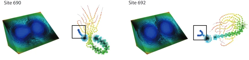
[image:2.612.89.523.146.252.2]Site 690 Site 692
Fig. 1. Scission point: A single plutonium nucleus (left) breaks into two fragments (right). Each image shows the iso-interval slabs within the 3D domain, and the abstract structure of the underlying Joint Contour Net.
Abstract—In nuclear science, density functional theory (DFT) is a powerful tool to model the complex interactions within the atomic
nucleus, and is the primary theoretical approach used by physicists seeking a better understanding of fission. However DFT simula-tions result in complex multivariate datasets in which it is difficult to locate the crucial ‘scission’ point at which one nucleus fragments into two, and to identify the precursors to scission. The Joint Contour Net (JCN) has recently been proposed as a new data structure for the topological analysis of multivariate scalar fields, analogous to the contour tree for univariate fields. This paper reports the analysis of DFT simulations using the JCN, the first application of the JCN technique to real data. It makes three contributions to visualization: (i) a set of practical methods for visualizing the JCN, (ii) new insight into the detection of nuclear scission, and (iii) an analysis of aesthetic criteria to drive further work on representing the JCN.
Index Terms—Topology, scalar fields, multifields.
1 INTRODUCTION
Problems in science, engineering and medicine rarely involve just one property of a system. Simulations of combustion, turbulence, seis-mic movements, meteorology, astrophysics, and molecular physics all compute multiple properties simultaneously, such as temperature, pressure, velocity, vorticity, shear, combustion rate, and so on. To date, scientific visualization for such data has focused on techniques for representingindividualproperties. Visual exploration of multiple properties requires careful use of methods such as probing, glyphing, or multidimensional transfer functions. All of these approaches are ad hoc, relying on careful study and exploration to piece together a global understanding of the relationships from local, fragmented, models.
In physics, this problem is well illustrated by many-body systems such as molecules, atoms or nuclei where the system as a whole is the
• David Duke and Hamish Carr are with the School of Computing,
University of Leeds, UK, E-mail:{D.J.Duke, H.Carr}@leeds.ac.uk.
• Aaron Knoll is with Argonne National Laboratory, USA, E-mail:
• Hai Ah Nam is with Oak Ridge National Laboratory, USA, E-mail:
• Nicolas Schunck is with Lawrence Livermore National Laboratory, USA,
E-mail: [email protected].
• Andrzej Staszczak is with the Department of Theoretical Physics,
University Marie Curie-Skłodowska, Lublin, Poland, E-mail: [email protected].
Manuscript received 31 March 2012; accepted 1 August 2012; posted online 14 October 2012; mailed on 5 October 2012.
For information on obtaining reprints of this article, please send e-mail to: [email protected].
product of complex interactions among many constituents, the prop-erties of which may not be easily isolated. In this paper, we focus on nuclear fission, the process by which an atomic nucleus splits into two (or more) fragments. Although it was discovered more than 70 years ago, physicists are still working on a comprehensive description of this complex phenomenon. One goal is to replace current phenomeno-logical models with a predictive model grounded in the theory of the strong interaction. This would yield deeper insight into the formation of elements in the universe, and also help address pressing societal questions related to energy production or stockpile stewardship [27].
A particularly challenging aspect within the theory of fission is the ability to identify accurately, in a continuousN−dimensional mani-fold, the points where the original nucleus ceases to be whole, and where it is justified to introduce two separate density distributions cor-responding to the fission fragments. This identification is convention-ally done manuconvention-ally and relies on the physicists’ intuition rather than clear mathematical arguments. By nature, however, this problem is an excellent candidate for multifield analysis.
Recent work [8] sets out a clear mathematical basis for multifield analysis: the Joint Contour Net (JCN). JCNs generalise the Contour Tree (and Reeb Graph) from one to an arbitrary number of scalar properties. Underlying this approach is a key assumption: that, by visualizing the JCN it will be possible to gain global insight into the relationship between the fields, and/or to identify important changes in the topological structure of the full system in terms of features in the JCN. This has been demonstrated on small synthetic datasets, but not yet on real data linked to a specific scientific problem.
This paper makes two principal contributions:
2. We demonstrate the utility of the JCN to real data, and explore the relationship between JCN analysis of multifields and contour tree analysis of single scalar fields.
The remainder of the paper is structured as follows. Section2 de-scribes nuclear density functional theory and its treatment of nuclear fission, introduces some useful vocabulary, and concludes with the key domain question addressed in this paper, namely finding the scission point in simulations of nuclear fission. These datasets are multivariate, and Sections3through5set out relevant formalisms and prior work including the JCN. Our visualization tools are described in Section6: these include implementation of the JCN, and methods for drawing it. The subsequent two sections,7and8, present our analyses of two substantial datasets. The first study, a simulation of fermium fission, serves to calibrate our approach. The second dataset, modeling fis-sion in the plutonium nucleus, is more challenging, and our analysis contributes new insight into physicists’ understanding of this system. Section9then reviews the contributions, and considers future research in this area.
2 NUCLEARFISSION INDENSITYFUNCTIONALTHEORY
Early models of fission were based on an empirical liquid-drop pic-ture of the nucleus: fission occurs when one “stretches” the drop up to the point where it breaks in two [4]. Modern approaches aim at deriving an understanding of the fission process from the nucleon-nucleon interactions that make atomic nuclei possible. In this con-text, the major theoretical approach is nuclear density functional the-ory (DFT) [2]. Its central assumption is that the complex interactions of protons and neutrons within the nucleus can be hierarchized. In first approximation, everything happens as if all nucleons were moving in-dependently of one another in some average quantum potential, the nuclear mean-field. Spontaneous symmetry breaking is invoked to de-form the mean-field, introducing a first class of correlations. Beyond this first order approximation, corrections are required to account for quantum fluctuations but the mean-field approximation alone is sur-prisingly successful: it typically accounts for 99.9% of the atomic mass of elements [19,20]. The DFT approach has three major ad-vantages over other approaches: (i) it provides a simple yet rigorous framework based only on an interaction between nucleons, (ii) it only depends on a handful of free parameters, and (iii) it is the only com-putationally tractable approach of the structure of heavy nuclei.
Because fission involves ‘stretching’ the nucleus, the DFT treat-ment of the problem begins with identifying the relevant deformation degrees of freedomqof the mean-field. A realistic description of fis-sion involves at least N≥4 degrees of freedom such as elongation, triaxiality, mass asymmetry, degree of necking, etc. [30,34]. The list of degrees of freedom defines what is called the “collective space”. The next task is to take a (not necessarily uniform) sample grid of thisN-dimensional collective space and compute the total energyEat each point of this grid. As the dimensionalityNof the collective space increases, the number of points may quickly become very large: high-performance computing is needed. The scalar fieldE(q1, . . . ,qN)
de-fines the “potential energy surface” (PES). At each point on the PES, the nucleus is characterized by properties such as the spatial density of protons and neutrons (scalar fieldR3→R), the density of spin of each type of particle (vector fieldsR3→R3), etc. A given set of such properties is nothing but a particular realization of a multifield.
The PES themselves are the cornerstone of the microscopic theory of fission. They have some topology with a minimum at small defor-mations, the “ground-state” of the nucleus, together with secondary minima, ridges and valleys. Starting from the ground-state and fol-lowing a path of least energy on the PES, we may observe at some point a discontinuity with a sharp drop of the energy: this defines the scission point, the precise moment where the nucleus fragments and can not be considered as whole any longer. To know precisely where the split occurs is essential in practical applications: it is what will de-fine the properties of the fission fragments, such as their charge, mass, kinetic energy and excitation energy; all quantities that can be mea-sured experimentally and test the predictive power of the model.
In many DFT simulations, the PES contains discontinuities and the identification of scission is therefore straightforward. Even then, se-rious conceptual difficulties arise because the properties of the fission fragments can change totally across the scission point precisely be-cause of the discontinuity. To avoid such inconsistencies, it is possible to remove all discontinuities by enlarging the collective space (adding new degrees of freedom to describe nuclear properties, see figure9): the properties of the fission fragments are then properly defined, but the identification of the scission point becomes much more compli-cated. We will show in this work that multifield analysis techniques are an effective tool to detect topological changes in such complex situations.
There are many other cases where these techniques could also prove very valuable for nuclear physicists. For example, the description of neutron-induced fission, e.g. in nuclear reactors requires adding ther-mal effects to the theory. As a consequence, nucleons tend to be more and more delocalized: densities extend further outside the nucleus and the definition of the scission point becomes more and more ambigu-ous, if not questionable. Apart from the identification of the scission point itself, perhaps as important is the detection of the nascent pre-fragments in the fissioning nucleus [28,29,35]. This is the signal that global degrees of freedom associated with the whole nucleus may have to be replaced by individual degrees of freedom for each frag-ment. Yet, there is currently no systematic way to perform this switch from global to local degrees of freedom, and multifield analysis offers an appealing option.
Since the task involves detection of a particular combinatorial event between distinct objects encoded in a multi-field composed of mul-tiple scalar fields, this problem is well-suited to topological analysis. Thus, in order to identify the scission points, we must first discuss the principles of topological analysis and visualization in the scalar case, then discuss multifield visualization and in particular the extension of topological analysis to multifield data.
3 SCALARTOPOLOGICALANALYSIS
In recent years, topological analysis has increasingly been applied to the analysis, visualization and comprehension of scientific data sets [6]. Two complementary approaches have been developed -contour-based analysis [10] and gradient-based analysis [14]. Of these, contour-based analysis detects objects and their relationships, while gradient-based analysis also detects regions of common be-haviour. At the same time, contour-based analysis is computationally cheaper and simpler than gradient-based analysis: we therefore start with scalar topological analysis using the contour tree.
5 9
1 8 8
5 6 7
4
3
4
6
7
8 9
3 2
1
3 8
4
3
7
5
6
1
2
9
3
9
5
1 2
4 6
7 8
7 8 9
4
1
5
2
6
3
9
[image:3.612.312.554.513.691.2]1
3.1 Contour Trees
Given a scalar fieldf:M⊂Rm→Rover a manifold domainM, a level
set f−1(h)is the pre-image of a given isovalueh, and a contour is a single connected component of a level set. We note that each contour is (on standard assumptions) of one dimension lower than the original data set, because we have restricted it with respect to one variable.
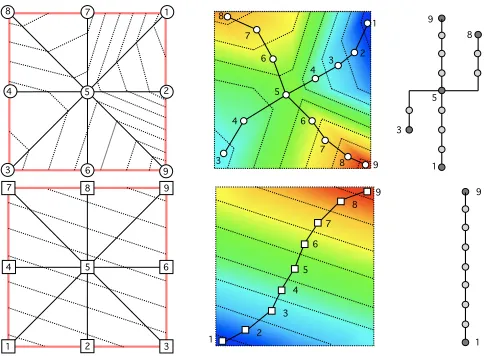
Contracting each contour to a single point results in a graph called the Reeb graph [23]. IfMis homeomorphic to a disk, this is the con-tour tree[5]: an example of a contour tree is shown in Figure2. In this figure, a small triangulated scalar field is shown with some contours (on the left), and a heat map to its right. Note that the contour tree captures the relationship between the maxima in red, the minima in blue, and the saddle point in the centre. All extrema are represented as leaf nodes and saddle points as interior nodes: all other points map to points on edges of the tree. Moreover, regions bounded by contours map to subsets of the tree, and branches of the tree therefore represent regions of the data.
The contour tree can be computed inO(NlogN)time for triangu-lated scalar fields [9], and has been used for feature detection [10], volume rendering [33], and contour extraction [10].
To compute contour trees and other topological abstractions, the first step is to reduce the input data to a combinatorial form, commonly a graph, for efficient algorithmic processing. This can be done through simplifying assumptions, which have the side effect of making compu-tations more complex. In particular, iffis defined by piecewise linear interpolation on a triangulated (simplicial) mesh [1] with no two vertex isovalues identical [15], computation can be performed on the graph defined by the edges of the input mesh. Alternately, graphs can be defined directly from digital image connectivity rules [21]. More re-cently, Forman’s Discrete Morse Theory [16] replaced gradient com-putation with a rigorous combinatorial approximation, allowing effi-cient approximation of the Morse-Smale Complex.
We will see in section5how to reduce multivariate data to a graph approximation called the contour net, but first review what multivariate data is and how it is visualized.
4 MULTIFIELDVISUALIZATION
Compared to a scalar field, a multifield can be thought of as a collec-tion of scalar fields with a shared domain or as a generalisacollec-tion of a scalar field to a multi-dimensional range: f:Rn→Rm. And, whileRn
is usually taken to be Euclidean space, bothRmandRnmay in general be continous parameter spaces. For example, a record of temperature, pressure, and humidity over the surface of the Earth defines a function
f :R2→R3, while a record of heat and gaseous concentration in a volumetric simulation of a plasma defines a functionf:R3→R2. We will consider each of the samples in the data domain individually to be scalar functions, i.e. we do not address the case where observations explicitly include vector or tensor components.
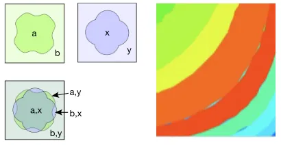
We can construct a small running example by combining the scalar field from Figure2with a second scalar field on the same domain in Figure2. If we combine the two to construct a functionf:R2→R2, we instantly run into the major problem with multifield visualization: how to construct separate visual encodings for each field. Figure3 illustrates this problem, with a heat map based on the sum of the two fields. Broadly speaking, multifield visualization is in its infancy, with methods that either reduce the multifield to a scalar field or map each element of the multifield to different visual channels.
5 MULTIFIELDTOPOLOGICALANALYSIS
As we have seen, successful tools have been developed for scalar topo-logical analysis. It has been an open question how to extend these tools to multifields, either by treating the properties as separate scalar fields, or by analysing the entire multifield at once. Moreover, re-cent work [11] has demonstrated that, for many purposes, quantized contours are a more appropriate form of analysis for the sampled and meshed data typical of scientific and engineering simulations. We therefore consider these three sets of research before proceeding.
Multiple Scalar Analysis:One approach has been to analyse each scalar field separately (e.g. in contour trees), then overlap the cor-responding features to determine which features are simultaneously represented in two fields [25]. Extending this to more than two fields, however, results in defining a graph of relationships between features in the scalar fields, then searching for cliques representing large over-lapping regions [24]. However, this approach only identifies features that are independently visible in each property.
Jacobi Sets:A second approach has been to generalise scalar topol-ogy to higher dimensions. A first step here was the introduction of Jacobi sets [12], which analyse the behaviour of critical points of one property on contours of another, but do not necessarily divide the do-main of the function into regions of full dimension that identify fea-tures in the data. More recently, Reeb graphs were extended to Reeb spaces [13] for multifields, but efficient practical algorithms have been lacking, in part due to the complexity of the Reeb spaces.
(3,1)
(4,1) (3,2)
(4,2) (4,3)
(5,2) (6,2) (7,2) (4,4)
(5,4) (6,5) (7,6) (8,7)
(7,7)
(6,6)
(5,5) (6,7)
(5,4)
(6,4)
(6,3) (7,4)
(8,3) (9,3) (3,5)
(1,8) (1,9) (4,9) (3,9) (2,9) (6,8)
(3,6)
1 2 3 4 5 6 7 8 9
1 2 3 4 5 6 7 8 9
First Field
Second Field
Fig. 3. Joint Contour Net for the small example. Left, the slabs af-ter merging and the Joint Contour Net shown dual to the slabs. Right, range-space placement: isovalues are mapped to(x,y)as in the contour tree(Figure2): where more than one node has a given isovalue, these are stacked perpendicular to the plane of the page (shown in colour).
Joint Contour Nets: Joint Contour Nets (JCN)s [7, 8] approxi-mate the Reeb space for sampled multivariate data. As with scalar topology, the first step is to reduce the data to a graph - in this case, based on quantization of the input data. Based on recent work on the relationship between histograms, sampling, isosurfaces and quan-tization [11], the Joint Contour Net is constructed in three stages. In the first, each cell of the mesh is explicitly subdivided along contours (isosurfaces) of the individual variables to decompose the domain into slabs of constant (quantized) values in each cell. In the second, the ad-jacency graph of the slabs is extracted: i.e. the graph representation of isovalued regions. Finally, adjacent slabs (in neighbouring cells) with identical isovalues are collapsed to compute the Joint Contour Net [8]. This representation then encapsulates the topological structure of the multifield at the chosen level of quantization. Moreover, varying the coarseness of quantization can be used to simplify the Joint Contour Net on demand, and the contour tree turns out to be a special case.
We illustrate this in Figure2and Figure3. In the simple case (a contour tree), we divide the scalar fields in Figure2along the contour boundaries shown to obtain a set of slabs, then extract the adjacency graph and collapse it as shown in the right half of the figure to obtain the contour trees of the individual scalar fields. If we wish to compute the Joint Contour Net for both variables, we simply intersect the slabs as shown in Figure3and obtain the Joint Contour Net shown therein.
[image:4.612.320.563.234.352.2]6 IMPLEMENTATION
In the previous sections, we identified that nuclear fission naturally gives rise to multi-variate data sets which lend themselves to topologi-cal analysis, and that the Joint Contour Net can potentially be applied. We therefore constructed an experimental visualization system to test this hypothesis, with two principal components - computation of the JCN and custom rendering using the Visualization Toolkit (VTK) [26].
6.1 Visualization Framework
Our visualization pipeline was implemented in version 5.8 of the Vi-sualization Toolkit (VTK) [26], taking advantage of VTK’s integrated support for both scientific and information visualization techniques, and adding a small number of custom filters:
• A filter that extracts the JCN with the algorithm described in
[7,8]. This takes a simplicial mesh as input, and produces two outputs, (i) a graph dataset encoding the topological structure of the network, and (ii) a set of 3D polyhedra (or 2D polygons) stored as an unstructured grid, representing the slabs.
• A filter for converting the unstructured polyhedral cells into
polygonal data that can be rendered.
• A filter for generating viewpoint-aligned (“billboard”) glyphs
that show, pointwise, the value of each component of a multi-scalar field. This filter is used in displaying the JCN, and is dis-cussed in detail later in this section.
The JCN filter used in this paper was implemented as a testbed for multifield topology, and has not been optimized for performance. For example, it explicitly generatesallof the slabs. While this capabil-ity was useful in the work reported here in relating the topological abstractions to the underlying physics, it is a significant performance bottleneck that will be addressed in subsequent work.
6.2 Drawing Joint Contour Nets
Trees and other networks from topological analysis are non-trivial for graph drawing. The (apparently) simple case of the contour tree is complicated as (a) the structure is anunrootedtree, and (b) in draw-ing the tree, there are often conflictdraw-ing aesthetics – e.g. vertical posi-tioning in 2D of nodes according to the isovalue of the corresponding contours, and horizontal positioning to reflect the branch hierarchy.
Topological structure can be shown by (i) positioning nodes in the underlying manifold, or (ii) positioning the structure in a separate space (usuallyR2orR3), as shown by Pascucci et al. [22], whose lay-out for contour trees inR3was inspired by orreries. Layout inR2is more difficult: Heine et al. [18] report an algorithm that uses heuristic search to reduce penalties arising from conflicting layout criteria. Nei-ther approach applies to the JCN, as both rely on properties of trees.
Absent a layout technique specific to JCNs, we have identified three generic methods that provide complementary insights into their struc-ture. Given a multifield function f:Rm→Rn,
Domain-space placementpositions each node at the centre of the cor-responding slab in Rm: an example of this can be seen in Figure3. Form≤3, the resulting layout can be visualized directly; form>3 some form of dimensional scaling will be required. Although simple to compute node positions while building the JCN, in our experience it is difficult to discern features via this layout, and in particular difficult to identify combinatorial events within a sequence of JCNs.
Range-space placementpositions nodes at the point inRndefined by
the threshold of the corresponding slab. This generalises the contour-tree drawing convention where CT node isovalue is mapped to one axis of the drawing space, and can be seen as a form of scatterplot, where samples in the data domain are connected by edges based on adjacency in the spatial domain. However, where two slabs have the same isovalue, the corresponding nodes will be co-located.
Force-directed placement: given the construction of the JCN from ad-jacent slabs, we expect these networks to have a mesh-like structure.
Prior work [17] has shown that force-directed layouts can be effective for such graphs, and these algorithms avoid the problem of co-located vertices. Although there are issues of scalability for larger graphs, for the datasets used in this study force-directed placement was found to be practical. Our graphs are laid out using vtkForceDirectedLayout-Strategy, an implementation within VTK of a spring embedder.
Having placed the nodes, the next challenge is to relate nodes to then-tuple of values for the corresponding slab. Our solution was a multi-variate glyph similar to pie glyphs [32], but adapted for multi-field scalar data. Geometrically, for ann-field dataset, each glyph is constructed by subdividing a circle intonsegments of equal area, and building a simple polygonal approximation to these segments. Each segment then corresponds to a single field value, and is rendered by colour-mapping that value through a standard VTK lookup table.
The remaining difficulty was to relate nodes in the JCN to slabs in visualizations of the spatial domain. For analysis of DFT data, we do not need to make exact matches; our concern rather was to correlate features in the topological structure with regions of the data. As an expedient approach, we used the fact that the surfaces were subject to interpolation shading. For the surface of a slab de-fined by(v1,v2, . . . ,vn), we randomly assign one of the scalar values
{v1,v2, . . . ,vn}to each vertex, and then pass the resulting single scalar
field through a colour map. We make no claims that this is a percep-tually good approach for multifield visualization in general, but for the specific task of identifying the scission point, it provided adequate support for relating the topological and spatial displays.
7 FERMIUMDATASET
Using datasets representing known fission pathways in fermium-258 [30], the primary aim of the first study was calibration: whether the visualization tools revealed behaviour knowna prioriby the physicists to be present, allowing the visualization members of the team to tune visual representation, and simplifying the task of understanding how the structure of the JCN relates to underlying physical phenomena.
Three datasets were provided by the physicists on the team for anal-ysis. Each dataset corresponded to a trajectory in the N-dimensional collective space defined in DFT, see section2. These were:
aEF:asymmetric elongated fission, where the fermium nucleus elon-gates asymmetrically, then splits into a large and a small fragment;
sCF:symmetric compact fission, where the fermium nucleus splits fairly abruptly into two approximately equal fragments, and
sEF:symmetric elongated fission, where the fermium nucleus elon-gates symmetrically.
Each of the trajectories is made of 56 sample points, or sites, corre-sponding to different values of the collective coordinates(q1, . . . ,qN).
At each site, three scalar fields on a regular 19×19×19 grid were gen-erated by the DFT solver. Data for each field was provided in “raw” format: 8-bit unsigned integers. The three fields used in this and the subsequent plutonium study are:
p:spatial density of protons in the nucleus,ρp(x,y,z);
n:spatial density of neutrons,ρn(x,y,z);
t: spatial density of nucleons (protons and neutrons); ρt(x,y,z) =
ρn(x,y,z) +ρp(x,y,z)
As discussed in section2, the conventional approach to detecting the scission point relies on looking for evidence of a sudden drop in the energy. In figure4, such a drop is clearly visible for the aEF trajec-tory; for sCF, there seems to be a change of slope rather than a genuine discontinuity; finally, for sEF, only a gradual decline in energy is visi-ble, and, from the figure alone, it is not certain if there is any scission point at all. This information was not provided by the physicists prior to application of the JCN.
7.1 Protocol and Interpretation
0 100 200 300 400 500 -1980
-1960 -1940 -1920 -1900
258
Fm
(SkM*)T
o
ta
l
e
n
e
rg
y
E
to
t (
M
e
V
)
Quadrupole moment Q20 (b)
sCF sEF aEF
Apparent change in slope for sCF sCF scission as
detected by JCN
[image:6.612.134.481.59.192.2]aEF scission as detected by JCN
Fig. 4. Parameter space for fermium-258 fission (adapted from Bertsch et al. [3]). On the left, an energy landscape with three trajectories plotted and isosurface visualisations along each trajectory. On the right, energy plots along the specific trajectories studied (adapted from Staszczak et al. [31]). The JCN identified no scission in sEF, scission in aEF at the site marked, and scission in sCF several sites sooner than the energy plot would indicate.
trajectories given. Based on experimentation, we adjusted the param-eter settings of the vtkForceDirectedLayoutStrategy filter to use 750 iterations per layout, an initial temperature of 12.0, and a cool-down rate of 5. Other parameters were left at their default setting.
Clearly an important question is the choice of slab width used to construct the JCNs. Since the data domain consists of 8-bit samples, we started with a slab width of 32, then reduced the width to 16, 8 and 4. For combinatorial events in the fermium dataset, we found widths 16 and 8 sufficient to identify the combinatorial events; reducing slab width to 4 did not add further insight, and incurred significantly greater running time due to the size of the resulting graphs; as an illustration, for sample point 47 on the aEF trajectory, width 32 results in|V|=20,
|E|=19; width 16 gives 407 and 773, width 8 gives 877 and 1708, while width 4 has 2553 and 5048 respectively.
Before reporting the results of our analyses, we use the example in Figure5to introduce and explain the output produced by our visual-ization pipeline. We have arbitrarily selected sample points 20 and 38 along the sCF trajectory, at slab widths 16 and 8. The left hand side of each figure shows the 3D arrangement of the polyhedra defined by the slabs of constant value, exposed by a cutting-plane. The right hand figure shows the corresponding JCN.
a
b
x
y
a,x
b,y a,y
b,x
Fig. 6. Interpreting star-like motifs: (left) schematic of slab-edge bound-aries, (right) 2D slice through dataset, coloured by slab identifier. Here
a&bare the values of the first field defining its slab boundaries, whilex
&yare slab boundary values for the second field.
Several features stand out in these images: the ‘shell-like’ arrange-ment of slabs within the 3D geometric representation, and the recur-ring chains of star-like ‘motifs’ within the JCNs. Interpreting the shell-like structures is straightforward: nucleon densities are highest at the centre of the dataset grid, and fall off towards the edges of the domain, taking their minimum value at the eight corner points. This interpre-tation is further supported by contour trees generated from thepand
nfields individually, which displayed eight ‘strands’. With respect to the star-like motifs, we noted the following:
1. The centre of the star corresponds to two high-degree nodes, most of whose neighbours are the low-degree nodes making up the remainder (‘fringe’) of the star.
2. Scaling glyphs according to slab triangle count shows that star centers correspond to ‘large’ slabs, and fringes to ‘small’ slabs. While layout filter parameters affect the aesthetic quality of the JCN drawing, it does not significantly alter the star-like features, i.e. these are not artefacts of the layout. Rather, given the topological structure of these subgraphs, the star-like appearance is a consequence of the spring embedder layout, which tends to cluster low-degree peripheral vertices around more central nodes. More importantly, given the shell-like geometric structures resulting from quantisation of thep andn
fields into slabs, we hypothesised that the ‘stars’ were the result of interference-like effects: where ap-shell and ann-shell boundary are in close proximity, overlaps between the fields result in small regions where one or both of the field values cross into the next slab interval; this structure is shown in Figure6(left). This was confirmed by taking a 2D slice through the data and colouring the field by slab-id. Figure6 (right) shows small slabs lying at the boundary between larger slabs (the degree-2 fringe nodes; the degree-1 nodes in the JCN ‘fringe’ are slabs that are fully contained within another).
With this understanding of the link between the JCN and underly-ing data, Figure5shows an example of an interesting combinatorial event. The JCN from position 20 is suggestive of one chain of ‘shells’ with embedded fragments; in contrast, the JCN at site 38 has a bi-furcated structure. The colour mapping shows that the two ‘ends’ of the bifurcation corresponded to shells within the centre of the dataset, and further inspection of these suggested the formation of two sepa-rate inner structures. The first image (site 20) therefore represents a nucleus before scission, and latter image corresponds to a point be-yond scission, where the two fragments are clearly separated. Note that, while in this case the separation might have been identified by judicious placement of the cutting plane, in the general case scission may give rise to multiple fragments.
7.2 aEF: asymmetric Elongated Fission
[image:6.612.77.282.488.594.2]Width 16 Site 20
Width 8 Site 20
Width 16 Site 38
[image:7.612.96.522.61.238.2]Width 8 Site 38
Fig. 5. Example JCNs from the sCF dataset, showing variation both in resolution (slab width) and along a trajectory.
Site 44 Site 45
Site 46 Site 47
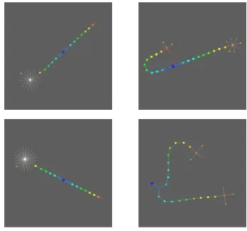
Fig. 7. Scission point in the aEF dataset. Starting from site 44, site 45 shows a break in local symmetry, persisting in site 46. Site 47 shows wholesale change, with the central ‘spine’ of the topology split into two branches.
7.3 sCF: symmetric Compact Fission
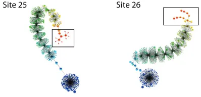
The sCF dataset was an effective test of the JCN: scission occurs, but identification of the scission point is not straightforward. In the output images, a significant topological shift is visible between site 25 and site 26, as shown in Figure8. Site 25 from the sCF resembles site 46 in the aEF, but there is no corresponding feature like site 26 in the aEF. The aEF fission pathway was abrupt, showing an immediate branch-ing into two fragments, whereas the sCF fission pathway is smooth, with site 26 showing the first indications of branching. This was pro-posed as the scission point, and subsequently confirmed by the physi-cists to be the start of the fission pathway. Notably, the markers of scission are visible through the JCN on the trajectorybeforeit shows up in the energy plot of Figure4. As described in section2, this infor-mation could provide a systematic marker for when global and local degrees of freedom should be applied to the model, and will be further investigated in future work.
7.4 sEF: symmetric Elongated Fission
In the sEF, initial analysis of the JCN at slab width 8 failed to iden-tify a definite scission point, although changes in the ‘backbone’ of
[image:7.612.326.525.281.377.2]Site 25 Site 26
Fig. 8. Scission point in the sCF dataset. The tail of the dataset (site 25) has split into two clearly-defined strands in site 26.
the structure suggested that fragments were organizing into discernible strands that could be precursors to fission. However, visual inspection at finer granularity (smaller slab width) still failed to identify any clear fission point, and this was reported to the physicists. This was actu-ally the correct conclusion to draw from the data: the physicists had deliberately posed sEF to see if the JCN would return a false positive. In fact, the sEF trajectory provided does not include a scission point, and the ‘failure’ to identify such a point via the JCN added further confidence in the utility of the multifield analysis.
8 PLUTONIUMDATASET
The spontaneous fission of fermium nuclei confirmed the validity of the JCN to identify scission. We now consider plutonium (Pu) fission: abundant in the spent nuclear fuel generated by nuclear reactors, its properties have been the focus of numerous experiments. Physicists’ understanding of its fission process is thus far more detailed than in the more exotic fermium superheavy element. Figure9shows the total en-ergy along the trajectory that minimizes the enen-ergy in a 4-d collective space (“most probable fission”). The discontinuity signaling the scis-sion point is clearly visible for an elongationQ20=345.
As mentioned in section 2, while discontinuities in the PES are useful to identify unambiguously the scission point, they prevent the proper characterization of the fission fragments. A solution consists in adding one or several degrees of freedom to the DFT description such that the pre- and post-scission points will be connected through a con-tinuous path. The right panel of figure9illustrates this scenario: for the value of the elongation characteristic of scission (as seen in the left panel), we show the variation of the energy as a function of the number of particlesQNin the “neck” of the nucleus, i.e., in between the two
[image:7.612.63.261.281.472.2]100 Q200 300 400
20 [b]
-30 -25 -20 -15 -10 -5 0 5 10 15
De
for
ma
tio
n E
ner
gy
[M
eV]
0.0 1.0 2.0 3.0
4.0 Number of particles in the neck Q
N
-20 -15 -10 -5 0
De
for
ma
tio
n E
ner
gy
[M
[image:8.612.63.301.55.123.2]eV]
Fig. 9. Total energy of isotope240Pu as a function of elongationQ 20(left) and number of particles in the neckQN(right).
Post-scission (Q =0.4)
Pre-scission (Q =0.5)
N
[image:8.612.57.301.190.342.2]N
Fig. 10. Scission inQNfield: note how the JCN clearly shows the split,
where conventional visualizations are ambiguous.
size of the neck. The important consequence of adding this extra con-straint is that what was a discontinuity in a 4-d space (transition from
Q20=345 toQ20=346 in the left panel) becomes a continuous path
in the 5-d space, as evidenced in the right panel of the figure. The only criterion that physicists could use to identify scission unambiguously, namely the discontinuity in the energy, has disappeared. Yet, analy-sis of the physics characteristics shows that atQN≥4, the nucleus
is whole, and atQN≤0.1, it has split in two fragments, so scission should occur somewhere in between these two points.
The goal of the second study was therefore (i) to use multifield anal-ysis to locate the scission point alongboththeQ20andQNaxes, and
(ii) to investigate whether JCN analysis can shed light on the rela-tionship between these fields and the structural changes within the Pu nucleus, e.g. identifying subtle differences in the behavior of neutron and proton density fields.
For the plutonium dataset, the trajectory shown in the left panel of figure9is made of 669 sites along theQ20axis. As for fermium, each
site along the trajectory corresponded to a 3-field (p, n, andt) vol-umetric dataset, in this case with dimensionality 40×40×66. This data came from a different source to the fermium, and underwent pre-processing including negative log transformation, as there were con-cerns that the gradient in regions of the data would be problematic for JCN analysis. A consequence of the transformation used was that the sense of field density was changed, with the higher density regions mapping to lower values in the 8-bit fields. This inversion was elimi-nated from processing of later samples, but explains why the sense of the density field is flipped between Figure 1 and other images. Analy-sis of the dataset was carried out with increasingly fine slab granular-ity. An initial sweep at slab width 32 failed to identify any combina-torial event, but sampling the dataset at resolution 16 showed a bifur-cation appearing between sites 650 and 740; further analysis down to slab width 8 confirmed that the split appeared between sites 690 and 692 (Q20=345). This transition is shown in Figure 1, and corresponds
exactly to the physics interpretation of the left panel of figure9.
The right panel of Figure9corresponds to a trajectory with 45 sites along theQNaxis. A sweep through the data at resolution 8 indicated
clearly a discrete point where the multifields topology underwent a significant change. Figure10shows the two sitesQN=0.4 andQN=0.5
on either side of the transition. This putative scission point differs somewhat from that expected by the physicists (for example, scission was assumed to have occured atQN≤1.0 in [34]), but the situation is in fact more complicated. Figure11shows three further points along theQNtrajectory, corresponding toQN=1.5, 2.5, and 3.5. Each JCN
has a branching structure: as the sequence progresses, the “neck” be-comes progressively larger. The event in Figure11 is thus only the point where the neck completely disappears, leaving the density fields for two fragments enclosed only by the simulation bounds. This marks one end of a scissionregion, which starts when the bifurcation first ap-pears.Thus, instead of simply identifying one combinatorial event rep-resenting scission, the JCN analysis unexpectedly revealed that scis-sion itself is a process occupying a region within the collective space.
[image:8.612.321.561.234.328.2]Site 15 (Q = 1.5)N Site 25 (Q = 2.5)N Site 35 (Q = 3.5)N
Fig. 11. Elongation of the neck region in the JCN: see text for discussion.
The final point addressed is the relative utility of the JCN compared to contour trees of individual fields. Figure12shows contour trees for
pandnfields and slab resolutions 16 and 8 for the sites atQN=0.4
and 0.5 (either side of the end of the scission region). Although taken individually the contour trees are simpler, the different properties of protons and neutrons mean that neither field on its own provides an unambiguous signal that the scission region has ended.
Fig. 12. Contour trees for thep(left column) andn(right column) fields around the Pu scission point. Top row:QN= 0.4 for slabs 16 (left) and 8
(right); Bottom row:QN= 0.5 for slabs 16 (left) and 8 (right)
9 CONCLUSIONS
We set out with the intention to demonstrate the utility of JCN analy-sis in multifield data, and to provide visualization support for nuclear physicists in determining scission points in high-dimensional parame-ter spaces. In the outcome, we succeeded in showing that:
[image:8.612.354.527.441.603.2]2. The JCN gives a more precise answer than hitherto available to the fundamental question of when scission occurs, and in fact shows that scission does not necessarily occur at points of inflec-tion in the energy plots,
3. Moreover, the JCN provides evidence that scission is best viewed as aregionrather than a discrete point,
4. While the contour tree also answers this question, the JCN does so more reliably, and at lower levels of quantisation,
5. Star-like structures can be expected to occur in the JCN, but pri-marily represent aliasing at the boundary of quantization inter-vals, and can therefore be disregarded,
In future, we intend to explore both the underlying JCN represen-tation and its applications to nuclear physics and other domains. As with previous topological representations, we would like to relax the current requirement of simplicial meshes, to consider improved algo-rithms for computing the JCN, to simplify it, and to recognize features in it automatically. We also intend to explore the meaning of motifs in the JCN: we suspect, for example, that the star-like artefacts noted in this paper are related in some way to the phenomenon of aliasing. Further research is also likely to improve visualizations of the JCN, and to build new visualization tools based on features detected in it.
With respect to the nuclear physics, a number of directions are also feasible. In particular, since the simulations come from wave-functions, particles may be localized in both fragments due to many-body quantum entanglement [35]. We believe that it may be possible to apply multifield techniques directly to the wave functions rather than to the total density of nucleons, and thus provide a criterion as to their degree of localization (left, right, everywhere).
ACKNOWLEDGMENTS
This work was partly performed under the auspices of the U.S. Depart-ment of Energy by Lawrence Livermore National Laboratory under Contract DE-AC52-07NA27344, and by Oak Ridge National Labora-tory under Contract DE-AC05-00OR22725 with UT-Battelle. Fund-ing was also provided by the U.S. Department of Energy Office of Science, Nuclear Physics Program pursuant to Contract DE-AC52-07NA27344 Clause B-9999, Clause H-9999, and the American Re-covery and Reinvestment Act, Pub. L. 111-5. Support was also pro-vided by the UK Engineering and Physical Sciences Research Coun-cil under Grant EP/J013072/1 and by the National Science Center (Poland) under Contract DEC-2011/01/B/ST2/03667.
REFERENCES
[1] T. Banchoff. Critical points and curvature for embedded polyhedra. J.
Diff. Geom, 1:245–256, 1967.
[2] M. Bender, P.-H. Heenen, and P.-G. Reinhard. Self-consistent mean-field models for nuclear structure.Reviews of Modern Physics, 75:121, 2003. [3] G. Bertsch, D. Dean, and W. Nazarewicz. Computing atomic nuclei.
SciDAC Review, Winter:42–51, 2007.
[4] N. Bohr and J. Wheeler. The mechanism of nuclear fission. Physical
Review, 56:121, 1939.
[5] R. L. Boyell and H. Ruston. Hybrid Techniques for Real-time Radar Simulation. InProceedings of the 1963 Fall Joint Computer Conference, pages 445–458. IEEE, 1963.
[6] P.-T. Bremer, G. Weber, V. Pascucci, M. S. Day, and J. Bell. Analyzing and Tracking Burning Structures in Lean Premixed Hydrogen Flames.
IEEE Transactions on Visualization and Computer Graphics, 16(2):248–
260, 2009.
[7] H. Carr and D. Duke. Joint contour nets: Topological analysis of mutli-variate data. InVisWeek Poster Compendium. IEEE, 2011.
[8] H. Carr and D. Duke. Joint contour nets: Topological analysis of mutli-variate data. In review at IEEE Transactions on Visualization and Com-puter Graphics, 2012.
[9] H. Carr, J. Snoeyink, and U. Axen. Computing Contour Trees in All Dimensions. Computational Geometry: Theory and Applications, 24(2):75–94, 2003.
[10] H. Carr, J. Snoeyink, and M. van de Panne. Flexible isosurfaces: Sim-plifying and displaying scalar topology using the contour tree.
Computa-tional Geometry: Theory and Applications, 43(1):42–58, 2010.
[11] B. Duffy, H. Carr, and T. M¨oller. Integrating Histograms and Isosurface Statistics. IEEE Transactions on Visualization and Computer Graphics, 2012. In press.
[12] H. Edelsbrunner and J. Harer. Jacobi Sets of Multiple Morse Functions.
InFoundations in Computational Mathematics, pages 37–57, Cambridge,
U.K., 2002. Cambridge University Press.
[13] H. Edelsbrunner, J. Harer, and A. Patel. Reeb spaces of piecewise linear mappings. InProceedings of the twenty-fourth annual symposium on
Computational geometry, pages 242–250. ACM Press, 2008.
[14] H. Edelsbrunner, J. Harer, and A. Zomorodian. Hierarchical Morse Com-plexes for Piecewise Linear 2-Manifolds. InProceedings, 17th ACM
Symposium on Computational Geometry, pages 70–79. ACM, 2001.
[15] H. Edelsbrunner and E. P. M¨ucke. Simulation of Simplicity: A technique to cope with degenerate cases in geometric algorithms. ACM
Transac-tions on Graphics, 9(1):66–104, 1990.
[16] R. Forman. Discrete morse theory for cell complexes.Advances in
Math-ematics, 134:90–145, 1998.
[17] D. Harel and Y. Koren. Graph drawing by high-dimensional embedding.
InGraph Drawing, volume 2528, pages 207–219. Springer-Verlag, 2002.
[18] C. Heine, D. Schneider, H. Carr, and G. Scheuermann. Drawing contour trees in the plane.TVCG, 17(11):1599–1611, 2011.
[19] K. Kortelainen, T. Lesinski, J. Mor´e, W. Nazarewicz, J. Sarich, N. Schunck, M. Stoitsov, and S. Wild. Nuclear energy density optimiza-tion.Physical Review C, 82:24313, 2010.
[20] K. Kortelainen, J. McDonnell, W. Nazarewicz, P.-G. Reinhard, J. Sarich, N. Schunck, M. Stoitsov, and S. Wild. Nuclear energy density optimiza-tion: Large deformations.Physical Review C, 85:024304, 2012. [21] S. Mizuta and T. Matsuda. Description of the topological structure of
dig-ital images by region-based contour tree and its application.IEIC Tech-nical Report (Institute of Electronics, Information and Communication
Engineers), 104(290):157–164, 2004.
[22] V. Pascucci, K. Cole-McLaughlin, and G. Scorzelli. Multi-resolution computation and presentation of contour trees. InProc. Visualization,
Imaging, and Image Processing, pages 452–290. IASTED, 2004.
[23] G. Reeb. Sur les points singuliers d’une forme de Pfaff compl`etement int´egrable ou d’une fonction num´erique.Comptes Rendus de l’Acad`emie
des Sciences de Paris, 222:847–849, 1946.
[24] D. Schneider, C. Heine, H. Carr, and G. Scheuermann. Interactive Com-parison of Multifield Scalar Data Based on Largest Contours. Accepted
to Computer-Aided Geometric Design, 2012.
[25] D. Schneider, A. Wiebel, H. Carr, M. Hlawitschka, and G. Scheuermann. Interactive Comparison of Scalar Fields Based on Largest Contours with Applications to Flow Visualization.IEEE Transactions on Visualization
and Computer Graphics, 14(6):1475–1482, 2008.
[26] W. Schroeder, K. Martin, and B. Lorensen.The Visualization Toolkit: An
Object-Oriented Approach to 3D Graphics. Kitware, 2006.
[27] Scientific grand challenges: Forefront questions in nuclear science and the role of high performance computing, 2009. [Online; accessed 21-June-2012].
[28] J. Skalski. Relative kinetic energy correction to self-consistent fission barriers.Physics Review C, 74(5):51601, 2006.
[29] J. Skalski. Relative motion correction for fission barriers.Int. J. Modern
Physics E, 17:151, 2008.
[30] A. Staszczak, A. Baran, J. Dobaczewski, and W. Nazarewicz. Micro-scopic description of complex nuclear decay: Multimodal fission.
Physi-cal Review C, 80:14309, 2009.
[31] A. Staszczak, J. Dobaczewski, and W. Nazarewicz. Bimodal fission in the skyrme-hartree-fock approach.Acta Physica Polonica, B38:1589–1594, 2006.
[32] M. Ward and B. Lipchak. A visualization tool for exploratory analysis of cyclic multivariate data.Metrika, 51(1):27–37, 2000.
[33] G. Weber, S. Dillard, H. Carr, V. Pascucci, and B. Hamann. Topology-Controlled Volume Rendering. IEEE Transactions on Visualization and
Computer Graphics, 13(2):330–341, March/April 2007.
[34] W. Younes and D. Gogny. Microscopic calculation of 240Pu scission with a finite-range effective force.Physical Review C, 80:54313, 2009. [35] W. Younes and D. Gogny. Nuclear scission and quantum localization.