An evolutionary algorithm based on nash dominance for equilibrium problems with equilibrium constraints

promoting access to White Rose research papers

White Rose Research Online [email protected]

Universities of Leeds, Sheffield and York

http://eprints.whiterose.ac.uk/

This is an author produced version of a paper to be published in Applied Soft Computing.

White Rose Research Online URL for this paper:

http://eprints.whiterose.ac.uk/43283/

Paper:

Koh, ATM (2011) An Evolutionary Algorithm based on Nash Dominance for Equilibrium Problems with Equilibrium Constraints. Applied Soft Computing, (in press).

An Evolutionary Algorithm based on Nash Dominance

for Equilibrium Problems with Equilibrium Constraints

Andrew Koh

Institute for Transport Studies, 36-40 University Road, University of Leeds, Leeds, LS2 9JT, United Kingdom

Abstract

This paper introduces an evolutionary algorithm for the solution of a class of hierarchical (“leader-follower”) games known as Equilibrium Problems with Equilibrium Constraints (EPECs). In one manifestation of such games, play-ers at the upper level who assume the role of leadplay-ers, are assumed to act non cooperatively to maximise individual payoffs. At the same time, each leader’s payoffs are constrained not only by their competitor’s actions but also by the behaviour of the followers at the lower level which manifests in the form of an equilibrium constraint. By a redefinition of the selection crite-ria used in evolutionary methods, the paper demonstrates that the solution for such games can be found via a simple modification to a standard evolu-tionary multiobjective algorithm. We give a proposed algorithm (NDEMO) and illustrate it with numerical examples drawn from both the transporta-tion systems management literature and the electricity generatransporta-tion industry underlying the applicability of NDEMO in multidisciplinary contexts.

Keywords: Nash Equilibrium, Equilibrium Problems with Equilibrium Constraints, Transportation Systems Management, Electricity Markets

1. Introduction

A major trend in the provision of transportation services and facilities has been deregulation coupled with the private sector playing a larger role. When it occurs in highway [60] or transit [62], entities providing such services face competition from others with similar offerings. It is of interest to regulators

to understand how such organizations make decisions on their service levels in this deregulated environment.

In this environment, the service levels provided are an outcome of a non-cooperative Nash game [39] amongst the players. However in transportation, this game possesses a feature that distinguishes it from the classic Nash game: The players’ actions are constrained by a condition defining equilibrium in the transportation system [12]. Users of the transportation network make their route choice decisions by choosing routes that are the lowest cost according to Wardrop’s Equilibrium Principle [58] and their route choice is parameterized in the decision variables of these firms. Therefore this is a hierarchical (i.e. leader-follower) game with the firms as leaders at the upper level engaged in a Nash game and travelers as followers at the lower level routing according to an equilibrium condition. Thus the terms “firms”, “leaders” and “players” are synonymous in this context.

The game just described is an instance of a broader class of Equilibrium Problems with Equilibrium Constraints (or EPECs) ([35],[36]). EPECs have emerged as an area of research ([2],[10],[57]) in mathematics applicable to transportation systems management and other disciplines ([22],[36]). This paper focuses on the determination of equilibrium values of the strategic variables for each profit maximizing leader when in competition with others. This paper is an extension of the earlier work by the present author [29] but has been extended in two key areas. Firstly on the theoretical aspect, we strengthen the theoretical justification of the proposed algorithm. On the practical aspect, we demonstrate the applicability of our algorithm to the examples of EPECs that arise not only within transportation systems management but also those arising in the electricity generation industry to demonstrate that our proposed algorithm is indeed applicable in multidisci-plinary contexts.

The rest of this paper is organized as follows. In the next section we outline the literature of the leader follower game paradigm that forms the basis of this research. Section 3 subsequently focuses on the notions associ-ated with the non-cooperative Nash game underlying the behaviour of the leaders in the EPEC. Section 4 reviews both the deterministic (i.e. gradient based) and evolutionary approaches for computing NE. Section 5 elucidates the Nash Domination criteria developed in [33] and provides an algorithm. Section 6 presents numerical examples of the solution of EPECs utilizing the concept of Nash Domination. Section 7 concludes the paper with a summary and directions for further research.

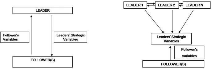
Figure 1: Stackleberg Game - Single Leader (MPEC)

Figure 2: Multiple Leader Follower Game (EPEC)

2. Leader Follower Games

Figure 1 gives a pictorial representation of what has come to be known as the Stackelberg game [56]. It is a model of the market structure whereby a single leader is able to gain increased profits by anticipating the reactions of the rest of the market participants (known as the “followers”). In the field of mathematics, the Stackelberg game is referred to as a Mathematical Program with Equilibrium Constraints (MPEC) and has been investigated in detail by a number of researchers (see [31],[41]). The characteristic unifying feature of MPECs is that in addition to general constraints, there exists a constraint specifying equilibrium in some parametric system. The key point to note is that the followers are assumed to take the single leader’s decision variables as exogenous when optimizing their individual objectives [32].

This equilibrium constraint is also present in the case of a Multiple Leader Follower Game shown in Figure 2. Though both models possess in common the hierarchical feature, the key difference between Figure 1 and Figure 2 is that multiple leaders are present in the latter and these leaders are assumed to play a game amongst themselves. We thus seek the equilibrium points of the game played by these upper level leaders. Hence as an extension of the MPEC, Figure 2 illustrates the more general class of Equilibrium Problem with Equilibrium Constraints (EPECs).

game amongst themselves resulting in a Non Cooperative EPEC (NCEPEC). In one of the numerical examples, we will revisit the distinction between the MOEPEC and NCEPEC. For the main part of this paper though we con-centrate exclusively on the situation in which leaders act non-cooperatively with the objective of maximizing personal gain.

Casting our present work within the broader research context, the exis-tence of the binding equilibrium condition distinguishes the games we de-scribe herein from standard Nash Games. In particular [12] have pointed out that the NCEPEC is a special case of a Generalised Nash Equilibrium Problem as described in (e.g. [19],[24],[52]).

3. Nash Equilibrium

Much of the game theory literature deals with games that are either zero sum where victory or gains for one player is exactly balanced by the defeat or losses for the other (as in games such as checkers [3]) or where the actions of players are constrained to be in a discrete set ( such as the binary options of confess/do not confess in games like the Prisoner’s Dilemma [49]). However the solution algorithms proposed for these are generally not applicable to NCEPECs. In such games, the payoffs to the players are continuous and the strategic decision variables are subsets of the real line (as described in Chapter 6 of [59]).

Consider the leaders’ problem in the NCEPEC. This is a single shot normal form game with a setN of players indexed byi∈ {1,2, ..., n}and each player can play a strategy si ∈Si which all players are assumed to announce simultaneously. S =

n

Q

i=1

Si is the collective action space for all players. It is convenient to denote s₋i as the combined strategies of all players in the game excluding that of player ii.e. s₋i ≡(s1, ..., s(i

−1), s(i+1), ..., sn) . So with

a slight abuse of notation, we have that s ≡ (si, s−i). We emphasize that

the notation (si, s−i)does not imply that the components ofs are reordered

such that si becomes the first block. We refer tos as a strategy profile of all players in the game. Let Ui(s) be the payoff to player i, i∈N if s is played.

Definition 1. [39] A combined strategy profile s∗ _{= (s}∗

1, s

∗

2, ..., s

∗

n) ∈ S is a

Nash Equilibrium (NE) for the game if :

Ui(s∗i, s∗−i)≥Ui(si, s

∗

−i) ∀si ∈Si ,∀i∈N (1)

Definition 1 emphasises the fact that at a NE no player can benefit (in-crease individual payoffs) by unilaterally deviating from its current strategy. Hence each player is doing the best taking into account what the competi-tors are doing [16]. The NE problem is the determination of strategies that satisfy Equation 1.

4. Computation of Nash Equilibrium

4.1. Deterministic Approaches

In a game, the optimal strategy for a player is governed by the best re-sponse function. If Ui(s) is continuously differentiable, then the best re-sponse function for player i is given by dUi(si, s−i)/dsi = 0 ([16], [59]).

The NE is the intersections of these best response functions for all players which amounts to finding solutions to n simultaneous equations i.e. solving

dUi(si, s−i)/dsi = 0,∀i∈ {1,2, ..., n} ([7],[59]).

While useful for providing insights into the behaviour of players, the an-alytical method is not feasible for realistic problems and even less so for NCEPECs due to the binding equilibrium condition. Thus the practical approach for finding NE is by using variants of fixed point iteration (e.g. non-linear Gauss-Siedel) ([25],[57]) or by formulating it as a Complemen-tarity Problem [26]. Applications of these methods are found in (e.g. [18], [30]). Convergence of these algorithms rely on the payoff functions being con-tinuously differentiable and possessing diagonally dominant Jacobians ([16], Theorem 4.1, pp. 280). However, if the payoff functions of the players are not concave, there may exist NE that satisfy Equation 1 locally but not globally. This is known as a “local NE trap” ([54], Definition 3, pp.306). There is thus a parallel with the literature on multi-modal function optimization where the potential for multiple optima cannot be ignored. Thus apart from their differentiability requirements, another drawback of deterministic approaches is that they can fall prey to the local NE trap, an occurrence crucially de-pendent on the starting point used in these algorithms. For details of these and other deterministic methods, see ([13],[14],[38]).

4.2. Evolutionary Methods

counterparts of deterministic fixed point iteration methods were proposed in ([48],[50] and [53]).

In particular, the motivation of the work reported in [53] was to employ the NE paradigm as an alternative to multiobjective optimization. In this work the authors provided an example which suggested that the NE point is on the Pareto Frontier which was generated by a standard evolutionary multiobjective optimization (EMO) algorithm. It was stated in [53] that the EMO required much more computing resources to generate the Pareto Frontier and the Nash Genetic Algorithm that these authors proposed would be robust for finding at least one solution and is hence useful as an alternative. However there is a need to exercise caution. Though there exists games where the NE is also Pareto Optimal, this is generally not the case. Since the NE fundamentally assumes non-cooperative behaviour between players with each maximizing personal rather than collective interests, it is clearly possible that one player can be made better off without making another worse off and thus in this case the NE is not Pareto Optimal. This fact has been demonstrated in [21] and will also be shown in a numerical example to be presented later in Section 6.

A parallel research strand has been the exploitation of co-evolution since it was first demonstrated [44] for tackling multi-dimensional function opti-mization. Several sub populations (one representing each problem dimension) are evolved simultaneously to avoid premature convergence and to widen the search of the problem space. Ideas from co-evolution have been exported into algorithms designed for the detection of NE; here each sub population encodes the strategies of individual players ([6],[43],[47]). However doubts have been cast on the performance of co-evolutionary methods. In [54], the co-evolutionary algorithm had to be hybridized with local search tech-niques to enable successful detection of NE. [27] developed a co-evolutionary particle swarm optimization method which attempted to detect the NE by learning the best response functions of the players. Instead of using the co-evolutionary paradigm of previous works, a novel idea exploiting the concept of Nash Dominance was proposed [33] to find NE as discussed in Section 5.

5. Nash Domination

5.1. Theoretical Foundations

At their most abstract level, evolutionary multi-objective (EMO) algo-rithms ([4],[11]) apply stochastic operators to a parent population with the

aim of evolving a fitter child population to solve vector valued optimiza-tion problems. Subsequently, in the selecoptimiza-tion phase, a comparison is made between a chromosome x from the parent population and a chromosome y

from the child population on the basis of fitness and the weaker of the two is discarded. This is entirely consistent with the principle of survival of the fittest. Given that one of the objectives of EMO is to identify the entire Pareto front [11], fitness is assigned based on Pareto Domination (PD): x

Pareto Dominates y if x is strictly no worse off than y in all objectives and

x is better than y in at least one objective ([11], Definition 2.5, pp. 28). [33] define a concept analogous to PD called Nash Domination for the NE problem. A chromosome in this context represents the strategies of allN

players concatenated into a row vector i.e. a strategy profile. Then instead of using PD to compare two chromosomes i.e. two strategy profiles, Nash Domination operates by counting the number of players that can benefit if each player switches strategiesin turn. Thefewer the number of players that can profit from unilaterally deviating from one profile compared to the other, the closer the former is to a NE following Definition 1.

Consider two strategy profiles{x, y} ∈S,(x≡(x1, ..., xn), y ≡(y1, ..., yn)) and introduce an operatork :S×S →N associating the cardinality of a set defined by 2:

{i∈ {1, ..., n} |Ui(yi, x−i)≥Ui(x), yi6=xi} (2)

The set thus defined by (2) comprises the players that would potentially benefit by playing yi when everyone else plays x−i. The total number of

players in this set is given by k(x, y). A similar interpretation applies, mu-tatis mutandis, for k(y, x). The procedure is summarized in Algorithm 1. Note that in order to evaluate k(x, y) and k(y, x), the payoff to each player, individually, from deviating has to be computed. Following this procedure outlined in Algorithm 1, one of the following outcomes must be true: ([33], Remark 4, pp. 365)

1. k(x, y)< k(y, x)→xNash Dominates y or

2. k(y, x)< k(x, y)→y Nash Dominates x or

3. k(x, y) = k(y, x) → x and y are Nash Non Dominated (NND) with respect to each other.

Algorithm 1 Nash Domination Comparison Initialize k(x, y) = 0, k(y, x) = 0

for i= 1 to n do

if Ui(yi, x−i)≥Ui(x) then k(x, y) =k(x, y) + 1

else if Ui(xi, y−i)≥Ui(y) then k(y, x) =k(y, x) + 1

end if end for

Proof. _{See [33], Proposition 9, pp. 366.}

The theoretical basis of the Nash Domination Comparison procedure pro-posed in [33] and outlined in Algorithm 1 is in fact founded on the Nikaido Isoda (NI) function. This function as given in Eqn. 3 is a mathematical tool that plays a key role in the study of NE problems [5],[12],[20],[24]. Consider again two strategy profiles {x, y} ∈ S, then the interpretation of Ψ(x, y) is as follows: each summand shows the increase in payoff a player will receive by unilaterally deviating and playing a strategy y while other players play according to x.

Ψ(x, y) = n

X

i=1

[Ui(yi, x−i)−Ui(x)] (3)

The interpretation of Ψ(y, x) is analogous: each summand in this case is the increase in payoff a player will receive by unilaterally deviating and playing a strategy x while other players play according to y. Ψ(x, y) is everywhere non-positive for all feasible y when x is a NE profile, a result that follows directly from Definition 1 because at a NE no player can increase their payoff by unilaterally deviating. Thus the NI function plays the role of a “merit function” measuring the proximity of a strategy to NE. In other words, the closer Ψ(x, y) when compared to Ψ(y, x), is to 0, the closer x is to a NE compared to y. Without explicitly using the NI function, the Nash Domination procedure suggested in [33] achieves the same goal by instead

counting the number of players that can profitably deviate.

5.2. The NDEMO Algorithm

Based on Lemma 1, we can find the NE by checking for Nash Dominance when comparing chromosomes. This replaces the usual Pareto Dominance check when using a standard EMO algorithm. Hence instead of locating the Pareto Front, we collect its analogue: the Non Nash Dominated Front to which the population converges. A proposed Nash Domination Evolution-ary Multiplayer Optimization (NDEMO) algorithm is given in Algorithm 2. NDEMO is based on the method of [51] which relies on Differential Evolu-tion (DE) [46]. By modificaEvolu-tion of this selecEvolu-tion criteria, any other EMO algorithm (see [4] or [11] for alternatives) can be used.

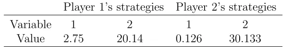
NDEMO operates as shown in Algorithm 2. The user specifies the max-imum number of iterations Maxit, the population size NP, the convergence tolerance, ǫ(>0), control parameters required in DE, namely Mutation Fac-tor F and Probability of Crossover CR [46] and a procedure to compute payoffs. Initial parent strategy profiles P are generated randomly. A hypo-thetical example of such a profile is shown in Table 1. Each chromosome is a vector in D dimensions with D being equal to the number of strategy vari-ables per player multiplied by the number of players (assuming that every player has the same number of strategy variables). In the hypothetical ex-ample given in Table 1 since there are two player with two strategic variables each, we have that D is 4.

Table 1: Example of chromosome encoding of a strategy profile in a hypothetical game with 2 players and 2 strategic variables per player

Player 1’s strategies Player 2’s strategies

Variable 1 2 1 2

Value 2.75 20.14 0.126 30.133

Algorithm 2 Nash Domination Evolutionary Multiplayer Optimization

1: Input: NP, Maxit, ǫ, DE Control Parameters, payoff functions

2: it←0

3: Randomly initialize a population of NP parent strategy profiles P

4: Evaluate payoffs to players with P

5: while it < Maxit orP not converged do

6: for j = 1 to NP do

7: use Algorithm 3 to create child strategy profiles vector y

8: Cit

j ←y

9: end for

10: Evaluate payoffs to players with C 11: T ← ∅

12: for j = 1 to NP do

13: x← P_jit

14: y ← Cit

j

15: use Algorithm 1 to carry out Pairwise Nash Domination Comparison between x and y to determine k(x, y) and k(y, x)

16: if k(x, y)< k(y, x) then

17: discardy

18: T ←x

19: else if k(y, x)< k(x, y) then

20: discardx

21: T ←y

22: else

23: T ←x

24: T ←y

25: end if

26: end for

27: if |T |> NP then

28: Randomly trim T until NP remain

29: end if

30: Randomly choose a chromosome m fromT

31: Compute Euclidean norm between m and every member in T

32: if maximum of norm ≤ǫ then

33: Terminate

34: else

35: P(it+1) ← T

36: it ←it+ 1

37: end if

38: end while

enforce bound constraints, we also utilise the method suggested in [45] (line 16 of Algorithm 3 ) so that if the child vector produced violates the bound constraints, it is reset to a point half way between its pre-mutation value and the bound violated.

Algorithm 3 Creating a child vector via Differential Evolution

1: Input: Current Population P

2: Input: Mutation Factor F, Probability of Crossover CR

3: Input: Lower Bounds LBd and Upper Bounds UBd in each dimension d

4: Randomly choose 3 integers: r1, r2, r3 between 1 and NP such that: 5: r16=j, r26=r16=j and r36=r26=r16=j,

6: x← Pj

7: a← Pr1

8: b ← Pr2

9: c← Pr3

10: Mutation: Produce a mutant vector z via a stochastic combination of donor vectors

11: z ←a+F(b−c)

12: for d = 1 toD do

13: Crossover

14: yd ←

zd

xd

if rand(0,1)< CR∨d=intr(1, D)

otherwise

15: Enforce Bound Constraints

16: yd ←

 



(xd+LBd)/2 if yd< LBd

(xd+UBd)/2 if yd> UBd

yd otherwise

17: end for

18: Output: child vector y

At each generation, parent and child strategy profiles are compared one by one pairwise, following the Nash Domination Comparison procedure of Algorithm 1. Those chromosomes that are NND are stored in a temporary population T. However, this means that the size of T, shown in line 27 of Algorithm 2 as |T |, may exceed NP. If this happens, we randomly trim T

less than ǫ, the population is judged to have converged to a NE and the algorithm can terminate. Otherwise the counter is increased and the process is repeated.

6. Numerical Examples

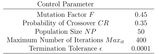
In this section six numerical examples occurring in three multidisciplinary contexts are provided to demonstrate the applicability of NDEMO to solving realistic problems. Table 2 gives the parameters used for the numerical exper-iments. Note that though we allowed for a maximum of 400 iterations, all the examples required less than this to meet the specified termination tolerance

ǫ of 0.0001. All numerical experiments were conducted using MATLABTM 7.8 running on a 32 bit WindowsTM _{XP machine with 4 GB of RAM.}

Table 2: Parameters used in the NDEMO for all Numerical Experiments

Control Parameter

Mutation Factor F 0.45

Probability of Crossover CR 0.35

Population SizeNP 50

Maximum Number of Iterations Maxit 400 Termination Toleranceǫ 0.0001

6.1. Examples from Production of Homogeneous Product

The first example presented arises when firms compete in the production of a homogeneous product. The purpose of this example is three fold. Firstly, we demonstrate that NDEMO successfully converges to previously reported results for games without any equilibrium constraint (i.e. when the game is not hierarchical in nature) and thus show that NDEMO can be applied to standard Nash games. Secondly, we use this example to demonstrate an instance of an MOEPEC when the players are assumed to cooperate. Finally, we wish to compare the solution of the MOEPEC with the NCEPEC for the purpose of emphasising the distinction between a non cooperative Equilibrium and a Cooperative Equilibrium.

The player dependent parameters (ωi, λi and θi) shown in Table 3 are found in [34]. These will be the parameters that we will use for the 3 case studies for this example.

Table 3: Production Cost Function Parameter Specification for Players

Firm i ωi λi θi

1 10 5 1.2

2 8 5 1.1

3 6 5 1.0

4 4 5 0.9

5 2 5 0.8

6.1.1. Case 1: Example 1 as a Cournot Nash Game

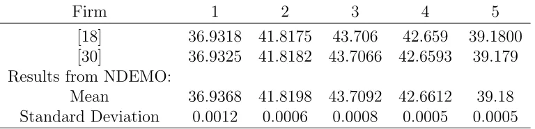
Here we consider the situation in which the firms engage in a Cournot-Nash game amongst themselves. Because of the absence of a hierarchical structure, this game is neither a NCEPEC nor a MOEPEC. However its in-clusion serves to demonstrate that the proposed algorithm is able to detect the NE and replicate the reported results in [18] and [30] where deterministic methods were proposed. In this setting, each firm maximises individual prof-its from the sale of the homogeneous good (given as the difference between revenues and production costs) as given by 4.

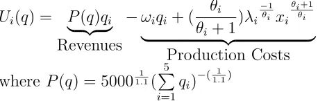
Ui(q) = P(q)qi

| {z }

Revenues

−ωiqi+ (

θi

θi+ 1

)λi

−1

θi _x i

θi+1 θi

| {z }

Production Costs whereP(q) = 500011.₁(

5

P

i=1

qi)−(

1 1.₁)

(4)

However the price (P(q)) and hence individual firm revenues is dependent not only on their on individual production levels but also on that of their competitors. Using the parameters of NDEMO as mentioned earlier, Table 4 reports results obtained from applying NDEMO to this problem and also compares it against the results published in the literature.

6.1.2. Case 2: Example 1 as a MOEPEC

Table 4: Example 1 Case 1 - Comparison of the Results of NDEMO with results published in literature

Firm 1 2 3 4 5

[18] 36.9318 41.8175 43.706 42.659 39.1800 [30] 36.9325 41.8182 43.7066 42.6593 39.179 Results from NDEMO:

Mean 36.9368 41.8198 43.7092 42.6612 39.18 Standard Deviation 0.0012 0.0006 0.0008 0.0005 0.0005

rise to a MOEPEC 1_{. Given the production levels of the leaders and treating}

these as exogenous, the followers seek to individually maximize their profits using 4. Assuming that the payoff functions are continuously differentiable (a condition easily verifiable for this example) the first order conditions for a profit maximum for each of the followers are defined by 5:

CP

 



fi = ∂U_∂qii ≥0

∂Ui ∂qiqi = 0

qi ≥0

 



i∈ {2,3,4} (5)

It is easy to see that 5 in fact defines a Complementarity Problem (CP) [13],[26],[30] which when written in generic form is to find q ∈ Rn _where

f :Rn→Rn such that:

f(q)≥0

qf(q) = 0

q≥0

(6)

As the leaders (firms 1 and 5) cooperatively maximise their profits, the actions of the followers leads to 5 which is imposed as an implicit nonlinear constraint on the leaders’ actions. The resulting MOEPEC can be written as a vector optimization problem (with T denoting the transpose) in 7.

1

This is in fact a MultiObjective Equilibrium Problem with Complementarity Con-straints (MOEPCC) but the MOEPCC is a special case of the MOEPEC and the distinc-tion does not affect our ensuing discussions.

max q1,q5

[U1(q1, q−1), U5(q5, q−5)]

T subject to

q1, q5 ≥0

{q2, q3, q4} →sol CP

(7)

In 7 “sol CP” emphasises that the production levels of the followers is the solution of the (nonlinear) CP given by 5. The Multiobjective Self Adaptive Differential Evolution (MOSADE) [23] algorithm was used to generate the Pareto Front corresponding to 7 and the resulting front is shown in Figure 3. In doing so, we integrated within MOSADE, the PATH Solver from [9] to solve the CP (i.e. 5) for each vector of the production levels of the leaders. On Figure 3, the two points marked with a ⋆correspond to the two solutions reported in [37] (see Table 5 ) which were obtained using a deterministic non smooth method. If negotiations between the leaders were allowed under prevailing anti-trust legislation, we conjecture that this Pareto Front would play a key role in these negotiations.

Table 5: The two solutions reported in [37] and indicated on Figure 3 with⋆

Solution 1 Solution 2 Profit of Leader 1/Firm 1 840.86 978.89 Profit of Leader 2/Firm 5 485.63 410.97

0 200 400 600 800 1000 1200 0

100 200 300 400 500 600 700

Profit: Leader 1

Profit: Leader 2

Figure 3: Example 1-Case 2 Pareto Front for MOEPEC

820 840 860 880 900 920 940 960 980 1000 380

400 420 440 460 480

Profit: Leader 1

Profit: Leader 2

Figure 4: Example 1-Case 3 The NCEPEC

6.1.3. Case 3: Example 1 as a NCEPEC

Using the same parameters as in the previous two cases, assume that these same leaders, firms 1 and 5 do not cooperate as they were assumed to do in Case 2 but instead play a Nash game amongst themselves. The optimization problem facing each leader individually is given in 8 and 9 respectively. As the leaders (firms 1 and 5) individually maximise their profits, the production levels of the followers leads to the complementarity problem which is imposed as an implicit nonlinear constraint on the leaders’ actions.

Player 1 /Leader 1

             max q1

U1(q1, q−1)

subject to

q1 ≥0

q5 = ¯q5

{q2, q3, q4} →sol CP

(8)

Player 5 /Leader 2

             max q5

U5(q5, q−5)

subject to

q1 ≥0

q1 = ¯q1

{q2, q3, q4} →sol CP

(9)

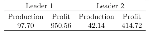
Critically compared to the MOEPEC, in the NCEPEC, when optimising their individual profits, each leader searches for the best response to the other firm’s production level. Integrating NDEMO with the PATH Solver [9] to resolve the CP as before, we apply NDEMO to solve the resulting NCEPEC. The result produced by the NDEMO algorithm is given in Table 6 and this solution (in profit space) is marked with×on Figure 4. As illustrated in Figure 4, the non cooperative outcome is not Pareto Optimal. It is obvious that any one of the leaders can be made better off (i.e. increase individual profits) without making the other worse off. For example, holding the profit from Leader 1 fixed at × of 950.56, one can move upwards (in the direc-tion of the arrow) towards the Pareto Front and hence increase the profit of Leader 2 without reducing the profit accruing to Leader 1. This outcome highlights the key difference between the MOEPEC and the NCEPEC and the proposed NDEMO algorithm is designed for the latter. Our finding is similar to that concluded in [21] 2 _{who also found that the result obtained by}

2

Figure 2 in [21] is analogous to Figure 4 in this paper.

the Nash Genetic Algorithm [53] lies inside the Pareto Front generated by a conventional EMO algorithm when optimizing a problem arising in the steel forging industry. In our example, the primary reason that the Nash point lies inside the Pareto Front is attributable to the assumption of non-cooperative behaviour between the leaders.

Table 6: Example 1 Case 3 - Production levels and Profits for Leaders in NCEPEC

Leader 1 Leader 2

Production Profit Production Profit 97.70 950.56 42.14 414.72

6.2. Examples from Private Sector Participation in the Operation of Toll Roads

The next three examples presented are typical of situations when pri-vate profit maximizing firms compete with one another in the operation of toll roads. The private firms, acting as leaders, set their strategic decision variables and the followers (who are in effect the highway users) optimize their route choice according to Wardrop’s Equilibrium Condition [58]. We seek therefore to compute the Nash Equilibrium strategic variables of these games 3_.

We define the notation for a mathematical statement of the problem:

A: the set of directed links in a traffic network,

B: the set of links which are subject to tolls B ⊂A,

Q: the set of origin destination (O-D) pairs in the network,

v: the vector of link flowsv = [va]a∈A,

τ: the vector of link tolls with τa = 0,∀a6∈B,

c(v): the vector of monotonically non decreasing travel costs as a function of link flows on that link only,

c= [ca(va)]a∈A,

µ: the vector of generalized travel cost for each OD pair µ= [µq], q∈Q,

δ: the continuous and monotonically decreasing demand function for each O-D pair as a function of the generalized travel cost between OD pairqalone,

δ = [δq], q∈Q,

3

δ−1_{: the inverse demand function giving the highway travel cost as a}

function of the demands and

Ω: feasible region of flow vectors, defined by a linear equation system of flow conservation constraints.

For simplicity suppose that each player is able to set tolls only on a single link in the network then each seeks to maximize its individual revenue (payoff) as given in 10

Max τi

Ui(τ) =vi(τ)τi,∀i∈1,2...n (10)

Where vi is obtained by solving the variational inequality (11) i.e.

c(v∗_{, τ)}T_(v−v∗_)−δ−1_(δ∗₎T_(δ−δ∗_{)≥0, ∀(v, δ)∈Ω (11)}

Hence for a specified toll vectorτ, the solution of the Variational Inequal-ity defined by 11 results in a vector of link flows and demands (v∗_{, δ}∗ _{∈ Ω)}

that satisfies Wardrop’s Equilibrium principle [58] of route choice (see [8, 55]). It is well known that the variational inequality in 11 can be solved by means of a standard traffic assignment algorithm once the vector of tolls have been input [8].

6.2.1. Example 2

Figure 5: Highway Network with 18 directed links from [28] for Examples 1 and 2 (links labeled are road numbers)

This example is taken from [28]. Let roads number 7 and 10 shown in Figure 5 be the only toll roads operated by two independent players. This

Table 7: Example 2 - NCEPEC Tolls (seconds)

Firm Road NDEMO [27] [28]

1 7 141.36 141.36 141.37

2 10 138.28 138.29 138.29

example was solved as a complementarity problem in [28] and via a Coevo-lutionary Particle Swarm Algorithm in [27]. We employed NDEMO with the parameters given in Table 2 and NDEMO took 12 minutes to converge to the tolls shown in Table 7 which agrees with previous results. The standard deviation of the variables at convergence were both less than 0.0001.

6.2.2. Example 3

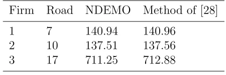
Next we consider the situation when, in addition to roads 7 and 10 be-ing tolled as in Example 2, another player maximizes payoffs by chargbe-ing tolls on road 17. The results are reported in Table 8. The standard devi-ation of the variables at convergence were both less than 0.0001. Although NDEMO again successfully converged to the NE (as verified by solving it as a complementarity problem following the method described in [28]), this time NDEMO took 19 minutes to meet the same convergence criteria. Thus with one additional player, the time taken has increased by 40% over the 2 player case. The increase in computing time stems from the domination checking procedure of Algorithm 1 combined with the hierarchical nature of the game. This arises from the need to solve a traffic assignment problem for each unilateral deviation (so as to obtain k(x, y) and k(y, x)).

Table 8: Example 3 - NCEPEC Tolls (seconds)

Firm Road NDEMO Method of [28]

1 7 140.94 140.96

2 10 137.51 137.56

Figure 6: Highway Network with 11 directed links from [60] for Example 3 (links labeled are road numbers), Dash lines indicate links (9,10 and 11) which are subject to Tolls and Capacity Expansion

6.2.3. Example 4

In this example we consider the 11 link network from [60] where each player has two strategic variables. In this case, beyond collecting the toll revenues, each player also has to finance capacity expansion of the network link operated. In addition to the notation introduced earlier, we redefineB to be the set of links which are subject to both tolls and capacity enhancements,

B ⊂A. Further letβrepresent the vector of link capacity enhancements with

βa = 0,∀a6∈B.

The payoff to player i, i∈N is the difference between the toll revenue obtained by collecting tolls from traffic using the link and the amortized cost of providing the capacity enhancements, I(βi). Thus α is a parameter that transfers the costs of the project into unit period costs. Mathematically, the resulting choice of the strategic variables for each player may be represented by the optimization problem in 12:

Max τi,βi

Ui(τ, β) =vi(τ, β)τi−αI(βi),∀i∈N (12)

Where vi is obtained by solving the variational inequality representing Wardrop’s User Equilibrium Condition (13)

c(v∗_{, τ, β)}T_(v−v∗_)−δ−1_(δ∗₎T_(δ−δ∗_{)≥0, ∀(v, δ)∈Ω (13)}

The three links (numbered 9,10 and 11) subject to tolls and capacity enhancements are shown as dashed lines in Figure 6. Details of the link pa-rameters and the functional forms of the travel demand relationships can be found in [60] where this was solved via a heuristic gradient based procedure.

The results in [60] are compared with those produced by NDEMO in Table 9. At convergence, the standard deviation of the population of toll and ca-pacity enhancement variables are all less than 0.0001. Although NDEMO took about 18 minutes to converge to the specified tolerance (which is simi-lar to the time taken in Example 2) this finding suggests that increasing the number of strategic variables per player did not have a significant effect on the performance of the algorithm.

Table 9: Example 4 - NCEPEC Tolls and Capacities

NDEMO [60]

Firm Link Toll Capacity Profit Toll Capacity Profit (secs) (vehicles) (secs/hr) (secs) (vehicles) (secs/hr)

1 9 4.53 151.74 302.04 4.52 151.60 301.43

2 10 4.76 193.01 417.63 4.76 193.04 417.14

3 11 2.97 61.29 25.98 2.97 61.88 25.92

We provide plots of the mean and standard deviation of the population at each iteration to illustrate the convergence of NDEMO for this problem. The left and right panes of Figures 7 to 9 show the means and standard deviation of the population of toll variables for each player over the 300 iterations of the algorithm. Similar plots are provided in Figures 10 to 12 of the population of the capacity variables for each player.

6.3. Examples from the Electricity Generation Industry

In deregulated electricity markets, electricity generating companies (“GEN-COs”) submit bids of the quantities of electricity they propose to supply to meet the market demand to maximize their profits. These bids are then cleared by the Independent System Operator (ISO). However the price and individual profits are not only dependent on their individual bids but also that of their competitors and the prices are not known until the market clear-ing is performed by the ISO [1],[15], [17]. This results in a NCEPEC and NDEMO can be applied to such “pool based bidding” games. The last two examples in this paper illustrate the performance of NDEMO in this context.

6.3.1. Example 5: Two Bus Model with 2 players

0 50 100 150 200 250 300 4 5 6 7 8 9 10 11 12 NDEMO Iteration

Mean of Tolls on Link 9 (Player 1)

0 50 100 150 200 250 300 0 1 2 3 4 5 6 7 NDEMO Iteration

Standard Deviation of Tolls on Link 9 (Player 1)

Figure 7: Example 4-Mean and Standard Deviation of Toll for Player 1 on Link 9

0 50 100 150 200 250 300 4 4.5 5 5.5 6 6.5 7 7.5 8 8.5 NDEMO Iteration

Mean of Tolls on Link 10 (Player 2)

0 50 100 150 200 250 300 0 1 2 3 4 5 6 NDEMO Iteration

Standard Deviation of Tolls on Link 10 (Player 2)

Figure 8: Example 4-Mean and Standard Deviation of Toll for Player 2 on Link 10

0 50 100 150 200 250 300 4 5 6 7 8 9 10 11 12 NDEMO Iteration

Mean of Tolls on Link 11 (Player 3)

0 50 100 150 200 250 300 0 1 2 3 4 5 6 7 NDEMO Iteration

Standard Deviation of Tolls on Link 11 (Player 3)

Figure 9: Example 4-Mean and Standard Deviation of Toll for Player 3 on Link 11

0 50 100 150 200 250 300 80 100 120 140 160 180 200 220 240 260 NDEMO Iteration

Mean of Capacities on Link 9 (Player 1)

0 50 100 150 200 250 300 0 20 40 60 80 100 120 140 160 180 NDEMO Iteration

Standard Deviation of Capacities on Link 9 (Player 1)

Figure 10: Example 4-Mean and Standard Deviation of Capacity for Player 1 on Link 9

0 50 100 150 200 250 300 180 185 190 195 200 205 210 215 220 225 NDEMO Iteration

Mean of Capacities on Link 10 (Player 2)

0 50 100 150 200 250 300 0

50 100 150

NDEMO Iteration

Standard Deviation of Capacities on Link 10 (Player 2)

Figure 11: Example 4-Mean and Standard Deviation of Capacity for Player 2 on Link 10

0 50 100 150 200 250 300 0 50 100 150 200 250 NDEMO Iteration

Mean of Capacities on Link 11 (Player 3)

0 50 100 150 200 250 300 0

50 100 150

NDEMO Iteration

Standard Deviation of Capacities on Link 11 (Player 3)

Ui(qi, q−i) =λ∗iqi −ci(qi), i∈ {1,2} (14)

Figure 13: Two bus network model from [54], Players 1 and 2 are located at G1 and G2 respectively.

However, as mentioned before, the prices λ∗

1, λ∗2 can only be determined

by the solution of a market clearing problem carried out by the ISO [15], [17]. Specific to the Two Bus Model shown in Figure 13 with player 1 and 2 located at buses G1 and G2 respectively, the ISO’s market clearing task is embodied in the solution of the system of equations in 15 for given bid submissions i.e. {q1, q2}.

max δ1,δ2,κ1

B1(δ1) +B2(δ2) (15a)

subject to

δ1−q1+κ1 = 0 (15b)

δ2−q2−κ1 = 0 (15c)

−TM ax _≤κ

1 ≤TM ax (15d)

The objective function 15a of the market clearing problem is maximization of the total benefits, the equality constraints in 15b and 15c represent Kirchoff’s Law and the inequality constraint 15d represents the transmission limits on the line. The prices, λ∗

1 and λ∗2, are given by the Lagrange multipliers of the

equality constraints in the market clearing problem 15b and 15c respectively. Within the scope of this paper it is the market clearing problem 15 that represents the equilibrium constraint facing each player which is a function not only of their own bids but also that of their competitor’s.

The benefit functions at each node/bus and the cost functions for each player from [54] are shown in Table 10. The line transmission limit TM ax _is 80. Table 11 compares the results from [54] with that obtained by NDEMO where 200 iterations were required to achieve the tolerance ǫ of 1e-4.

Table 10: Parameters of the Demand Function for Two Bus Model [54]

Bus/Player Benefit Function Bi(δi) Cost ci(qi) 1 −0.08(δ1)2+ 50(δ1) 0.01(q1)2+ 10(q1)

2 −0.04(δ2)2+ 30(δ2) 0.01(q2)2+ 10(q2)

Table 11: Example 5 - 2 Bus Model NCEPEC Bid Quantities (Megawatts/Hr)

Player 1 2

[54] 148 148

Results from NDEMO:

Mean 148.1267 148.1542

Standard Deviation 0.000289 0.000097

6.3.2. Example 6: Three Bus Model with 3 players

In this example, we consider the three player model from [7] and the 3 bus network used is shown in Figure 14. Three players submit bids to generate electricity to maximize individual profits from the generation of electricity according to 16.

Ui(qi, q−i) =λ∗iqi−ci(qi), i∈ {1,2,3} (16)

Once again the prices are determined by the market clearing problem given in 17. The equality constraints 17b, 17c and 17d represent the dc powerflow equations. The market clearing price tuple (the so-called loca-tional marginal prices) λ∗

i, i ∈ {1,2,3} is, as before, given by the Lagrange multiplier of these equality constraints. In this system of equations 17, θ1

and θ2 represent the powerflows on lines AC and -AC respectively. The last

constraint 17e is the transmission limit on the line.

max δ1,δ2,δ3

B1(δ1) +B2(δ2) +B3(δ3) (17a)

subject to

2θ1−θ2 =q1−δ1 (17b)

−θ1 + 2θ2 =q2−δ2 (17c)

−θ1−θ2 =q3−δ3 (17d)

−TM ax ≤κ1 ≤TM ax (17e)

The line transmission limit TM ax _{is 100 and the individual benefit} func-tions at each node/bus and the cost funcfunc-tions for each player are shown in Table 12 as reported in [7].

Table 12: Parameters of the Demand Function for Three Bus Model [7]

Bus/Player Benefit FunctionBi(δi) Cost ci(qi)

1 −0.0278(δ1)2+ 108.4096(δ1) 0.0079(q1)2+ 1.360575(q1) + 9490.366

2 −0.0335(δ2)2+ 103.8238(δ2) 0.0105(q2)2−2.07808(q2) + 11128.95

3 −0.0319(δ3)2+ 105.6709(δ3) 0.0065(q3)2+ 8.105354(q3) + 6821.482

Table 13 compares the results from [7] with that obtained by NDEMO where 300 iterations were required to achieve the tolerance ǫof 1e-4. Figures 15,16 and 17 show the mean and standard deviation of the population of each player’s bids, qi, i∈ {1,2}, over the iterations.

7. Conclusions

In this paper, we proposed modifying an evolutionary algorithm for solv-ing EPECs by extendsolv-ing the procedure suggested in [33]. The resultsolv-ing

0 50 100 150 200 250 300 800 850 900 950 1000 1050 1100 1150 NDEMO iteration

Mean of bids by player 1 (q

1

)

0 50 100 150 200 250 300 0 100 200 300 400 500 600 NDEMO iteration

Standard Deviation of bids by player 1 (q

1

)

Figure 15: Example 6-Mean and Standard Deviation of Bids for Player 1 on Bus 1

0 50 100 150 200 250 300 900 950 1000 1050 1100 1150 1200 NDEMO iteration

Mean of bids by player 2 (q

2

)

0 50 100 150 200 250 300 0 50 100 150 200 250 300 350 400 NDEMO iteration

Standard Deviation of bids by player 2 (q

2

)

Figure 16: Example 6-Mean and Standard Deviation of Bids for Player 2 on Bus 2

0 50 100 150 200 250 300 750 800 850 900 950 1000 NDEMO iteration

Mean of bids by player 3 (q

3

)

0 50 100 150 200 250 300 0 50 100 150 200 250 300 350 400 NDEMO iteration

Standard Deviation of bids by player 3 (q

3

)

Table 13: Example 6 - 3 Bus Model NCEPEC Bid Quantities (Megawatts/Hr)

Player 1 2 3

[7] 1105 1046 995

Results from NDEMO:

Mean 1105.396 1046.238 995.177 Standard Deviation 0.00104 0.00053 0.0008815

Nash Domination Evolutionary Multiplayer Optimization (NDEMO) algo-rithm enabled us to handle Nash games where players encounter a system equilibrium constraint. We highlighted the fact that the critical Nash Dom-ination procedure used in NDEMO to select between parent and child chro-mosomes is in fact theoretically rooted in the well established Nikaido Isoda function extending the original contribution of [33].

To assess the performance of NDEMO, six examples were given in this paper. The first,broken down into three case studies, used parameters from a well documented 5 player Cournot Nash model. The three case studies of the first example were given to underline the salient points of the market structure of competition assumed. In the first case study, we assumed that the players were competing non cooperatively but on an equal footing and this resulted in a standard Cournot Nash game for which NDEMO could be applied. In the second and third case studies, two players presented them-selves as “market leaders ” and this results in either the cooperative EPEC which is a MultiObjective Equilibrium Problem with Equilibrium Constraints (MOEPEC) (second case study) or the Non Cooperative Equilibrium Prob-lem with Equilibrium Constraints (NCEPEC) (third case study). The pro-posed algorithm, NDEMO, is designed for the latter case and conventional evolutionary multiobjective optimization (EMO) algorithms could be used for the former. This example highlights the difference between a MOEPEC and a NCEPEC, with the former arising from the assumption of coopera-tive behaviour amongst the leaders and the latter stems from assuming that the leaders engage in a Nash game amongst themselves. In both cases the strategies the leaders can play are subject to the actions of the followers which manifests in the form of an implicit nonlinear constraint on the actions of the leaders.

Three numerical examples illustrating competition in private sector par-ticipation in highway transportation and two examples drawn from pool

based bidding in the the electricity generation industry were further used to demonstrate the performance of NDEMO. In all instances, it was clear that NDEMO successfully converged to previously reported results in the literature and underscores the fact that the proposed algorithm is suitable for multidisciplinary applications.

While the examples suggest that this could be a potentially useful method for EPECs, we stress the need, in the pairwise comparison, to compute the payoff to each player, one by one, from deviating. This implies that the computational complexity of NDEMO increases significantly as the number of players increase as evidenced by the increase in computational times required in our examples. However, increasing the strategic variables available to each player did not significantly increase the time taken to solve the problem.

Further research would consider the effects of the control parameters of NDEMO on the speed of convergence to NND solutions. In this research we have used control parameters of the embedded Differential Evolution opera-tors suggested in [51]. Nevertheless these parameters are in no way regarded as perfect and it is hypothesized that well chosen parameters may reduce the run time of the NDEMO algorithm.

Acknowledgement

The research reported here is funded by the Engineering and Physical Sciences Research Council of the UK under the “Competitive Cities” Grant EP/H021345/1. The author would like to thank two anonymous referees for their comments and suggestions on improving the presentation of an earlier draft.

References

[1] Bower J., Bunn DW Model-Based Comparisons of Pool and Bilateral Markets for Electricity, Energy Journal 21(3), 1–29 (2000)

[2] ˇCervinka M: Hierarchical structures in equilibrium problems. PhD Thesis, Charles University, Prague, Czech Republic (2008)

[4] Coello-Coello C, Lamont G: Applications of multi-objective evolution-ary algorithms. World Scientific, Singapore (2004)

[5] Contreras J, Klusch M, Krawzyck JB Numerical solutions to Nash-Cournot equilibrium in electricity Markets. IEEE Transactions on Power Systems 19(1), 195–206 (2004)

[6] Curzon Price T: Using co-evolutionary programming to simulate strategic behavior in markets. Journal of Evolutionary Economics 7(3), 219–254 (1997)

[7] Cunningham L B, Baldick R, Baughman M L: An Empirical Study of Applied Game Theory: Transmission Constrained Cournot Behavior, IEEE Transactions on Power Systems 22(1), 166–172 (2002)

[8] Dafermos S C: Traffic Equilibrium and Variational Inequalities. Trans-portation Science 14(1),42–54 (1980)

[9] Dirkse S P, Ferris M C: The PATH solver: A non-monotone stabi-lization scheme for mixed complementarity problems, Optimization Methods and Software, 5 (2), 123-156 (1995)

[10] Ehrenmann A: Manifolds of multi-leader Cournot equilibria. Opera-tions Research Letters 32(2), 121–125 (2004)

[11] Deb K: Multi-objective optimization using evolutionary algorithms. John Wiley, Chichester (2001)

[12] Facchinei F, Kanzow C: Generalized Nash equilibrium problems. An-nals of Operations Research 175(1), 177–211 (2010)

[13] Facchinei F, Pang J S: Finite Dimensional Variational Inequalities and Complementarity Problems Volume 1. Springer, New York (2003)

[14] Facchinei F, Pang J S: Finite Dimensional Variational Inequalities and Complementarity Problems Volume 2. Springer, New York (2003)

[15] Gan D, Bourcier, D V: A single-period auction game model for mod-eling oligopolistic competition in pool-based electricity markets, IEEE Power Engineering Society Winter Meeting, 101–106 (2002)

[16] Gabay D, Moulin H: On the uniqueness and stability of Nash-equilibria in non cooperative games, In: Bensoussan A, et al, (eds) Applied Stochastic Control in Econometrics and Management Science. North Holland, Amsterdam, 271–293 (1980)

[17] Glover J D, Sarma M S, Overbye T, Power Systems Analysis and Design, Thomson: Toronto (2008)

[18] Harker P T: A variational inequality approach for the determination of Oligopolistic market equilibrium. Mathematical Programming 30(1), 105–111 (1984)

[19] Harker P T: Generalized Nash games and quasi-variational inequali-ties. European Journal of Operational Research 54(1), 81–94 (1991)

[20] Haurie A, Krawczyk J: Optimal charges on river effluent from lumped and distributed sources. Environ Model Assess 2(3), 177-189 (1997)

[21] Hodge B M, Pettersson F, Chakraborti N: Re-evaluation of the optimal operating conditions for the primary end of an integrated steel plant using multi-objective Genetic Algorithms and Nash Equilibrium, Steel Research International 77(7), 459–461 (2006)

[22] Hu X, Ralph D: Using EPECs to model bilevel games in restructured electricity markets with locational prices. Operations Research 55(5), 809–827 (2007)

[23] Huang, V L, Qin, A K, Suganthan P N, Tasgetiren M F:Multi-objective optimization based on self-adaptive differential evolution al-gorithm. Proceedings of IEEE CEC, 3601–3608 (2007)

[24] von Heusinger A, Kanzow C: Relaxation methods for generalized Nash equilibrium problems with inexact line search. Journal of Optimization Theory and Applications 143(1), 159–183 (2009)

[25] Judd K: Numerical methods in Economics, MIT Press, Cambridge,MA (1998)

[27] Koh A: Coevolutionary particle swarm algorithm for bi-level varia-tional inequalities: applications to competition in highway transporta-tion networks in Chiong R, Dhakal S(eds) Natural intelligence for scheduling, planning and packing problems. Springer, Berlin, 195–217 (2010)

[28] Koh A, Shepherd S: Tolling, collusion and equilibrium problems with equilibrium constraints. European Transport/Trasporti Europei 43:3– 22 (2010)

[29] Koh A: Nash Dominance with Applications to Equilibrium Problems with Equilibrium Constraints in Xiao-Zhi Gao, Antnio Gaspar-Cunha, Mario Kppen, Gerald Schaefer and Jun Wang (eds) Soft Computing in Industrial Applications: Algorithms, Integration, and Success Sto-ries, Advances in Intelligent and Soft Computing Volume 75 Springer Verlag: Berlin, 71–79 (2010)

[30] Kolstad M, Mathisen L: Computing Cournot-Nash equilibrium. Oper-ations Research 39(5), 739–748 (1991)

[31] Luo Z, Pang J, Ralph D: Mathematical Programs with Equilibrium Constraints. Cambridge University Press, Cambridge

[32] Leyffer S, Munson T: Solving multi-leadercommon-follower games. Op-timization Methods and Software 25(4), 601-623 (2010)

[33] Lung R I, Dumitrescu D: Computing Nash equilibria by means of evolutionary computation. International Journal of Computers, Com-mmunications and Control III, 364–368 (2008)

[34] Murphy F H, Sherali H D, Soyster A L: A mathematical programming approach for determining oligopolistic market equilibrium. Mathemat-ical Programming 24(1), 92–106 (1982)

[35] Mordukhovich B S: Optimization and equilibrium problems with equi-librium constraints. Omega 33(5), 379–384 (2005)

[36] Mordukhovich B S: Variational analysis and generalized Differ-entiation, II: Applications. Grundlehren der mathematischen wis-senschaften, Vol 331, Springer, Berlin (2006)

[37] Mordukhovich B S, Outrata J V, ˇCervinka M: Equilibrium problems with complementarity constraints: Case study with applications to oligopolistic markets. Optimization 56(4), 479–494 (2007)

[38] Nagurney A: Network Economics: A Variational Inequality Approach. Advances in Computational Economics, Kluwer, Boston (1999)

[39] Nash J: Equilibrium points in N-person games. Proceedings of the National Academy of Science USA 36(1), 48–49 (1950)

[40] Ortuzar J, Willumsen L: Modelling Transport. Wiley, Chich-ester(1990)

[41] Outrata J, Koˇcvara M, Zowe J: Nonsmooth Approach to Optimization Problems with Equilibrium Constraints. Kluwer, Boston (1998)

[42] Outrata J V: A note on a class of equilibrium problems with equilib-rium constraints. Kybernetika 40(5), 585-594

[43] Pedroso J P: Numerical solution of Nash and Stackelberg equilibria: an evolutionary approach. Proceedings of SEAL’96, 151–160 (1996)

[44] Potter M A, De Jong K: A cooperative coevolutionary approach for function optimization. In: Proceedings of PPSN III, Springer, Berlin, 249–257 (1994)

[45] Price K (1999), An Introduction to Differential Evolution in Corne D, Dorigo M, Glover F(eds) New Techniques in Optimization. London: McGraw Hill, 79–108.

[46] Price K, Storn R, Lampinen J: Differential evolution: a practical ap-proach to global optimization. Springer, Berlin (2005)

[47] Protopapas M, Kosmatopoulos E: Determination of sequential best replies in n-player games by genetic algorithms. International Journal of Applied Mathematics and Computer Science 5(1), 19–24 (2009)

[49] Rapoport A, Chammah A: Prisoner’s Dilemma. University of Michigan Press, Ann Arbour, Michigan (1965)

[50] Razi K, Shahri S H, Kian A R: Finding Nash equilibrium point of nonlinear non-cooperative games using coevolutionary strategies. Pro-ceedings of ISDA, 875–882 (2007)

[51] Robiˇc T, Filipiˇc B: DEMO: differential evolution for multiobjective problems. Proceedings of EMO2005, LNCS 3410,Springer, Berlin, 520– 533 (2005)

[52] Rosen J B: Existence and uniqueness of equilibrium point for concave N person games. Econometrica 33(3), 520–534 (1965)

[53] Sefrioui M, Periaux J: Nash genetic algorithms: examples and appli-cations. Proceedings of IEEE CEC, 509-516 (2000)

[54] Son Y, Baldick R: Hybrid coevolutionary programming for Nash equi-librium search in games with local optima. IEEE Transactions on Evo-lutionary Computation 8(4), 305–315 (2004)

[55] Smith M J The existence, uniqueness and stability of traffic equilibria. Transportation Research Part B 13(4),295–304 (1979)

[56] von Stackelberg, H H: The theory of the market economy. William Hodge, London (1952)

[57] Su C: Equilibrium problems with equilibrium constraints: stationar-ities, algorithms and applications. PhD Thesis, Stanford University, California, USA (2005)

[58] Wardrop J G: Some theoretical aspects of road traffic research. Pro-ceedings of Institution of Civil Engineers Part II, 1(36), 325-378 (1952)

[59] Webb J N: Game theory: decisions, interaction and Evolution. Springer, London (2007)

[60] Yang H, Feng X, Huang H: Private road competition and equilibrium with traffic equilibrium constraints. Journal of Advanced Transporta-tion 43(1), 21–45 (2009)

[61] Ye J J, Zhu Q J: Multiobjective optimization problem with vari-ational inequality constraints. Mathematical Programming Series A 96(1), 139–160 (2003)