A graph-based factor screening method for synchronous data flow simulation models

(1)

Rochester Institute of Technology

RIT Scholar Works

Theses

Thesis/Dissertation Collections

5-1-2009

A graph-based factor screening method for

synchronous data flow simulation models

Gregory Tauer

Follow this and additional works at:

http://scholarworks.rit.edu/theses

This Thesis is brought to you for free and open access by the Thesis/Dissertation Collections at RIT Scholar Works. It has been accepted for inclusion in Theses by an authorized administrator of RIT Scholar Works. For more information, please [email protected].

Recommended Citation

(2)

R

OCHESTER

I

NSTITUTE OF

T

ECHNOLOGY

A GRAPH-BASED FACTOR SCREENING METHOD FOR

SYNCHRONOUS DATA FLOW SIMULATION MODELS

A Thesis

Submitted in partial fulﬁllment of the

requirements for the degree of

Master of Science in Industrial Engineering

in the

Department of Industrial and Systems Engineering

Kate Gleason College of Engineering

by

Gregory W. Tauer

B.S., Industrial Engineering, Rochester Institute of Technology, 2009

(3)

D

EPARTMENT OF

I

NDUSTRIAL AND

S

YSTEMS

E

NGINEERING

K

ATE

G

LEASON

C

OLLEGE OF

E

NGINEERING

R

OCHESTER

I

NSTITUTE OF

T

ECHNOLOGY

R

OCHESTER

, N

EW

Y

ORK

C

ERTIFICATE OF

A

PPROVAL

M.S. D

EGREE

T

HESIS

The M.S. Degree Thesis of Gregory W. Tauer

has been examined and approved by the

thesis committee as satisfactory for the

thesis requirement for the

Master of Science degree

Approved by:

Dr. Michael E. Kuhl, Thesis Advisor

(4)

Abstract

This thesis develops a method for identifying important input factors in large system

dynam-ics models from an analysis based on those models’ underlying structures. The identiﬁcation

of important input factors is commonly called factor screening and is a key step in the

analy-sis of simulation models with many input parameters. Models under investigation are system

dynamics models implemented as synchronous data ﬂow programs, a model of computation

that requires encoding the model components’ dependencies in a graph format. The

devel-oped method views this graph as a stochastic process and attempts to rank the importance of

inputs, or source nodes, with respect to an output, or non-source node. This ranking is

accom-plished primarily through the use of weighted random-walks through the graph. A comparison

is made against other factor screening techniques, including fractional factorial experiments.

The presented structure-based method is found to be comparably accurate to statistical factor

screen experiments at magnitude order ranking. Run time of the developed method compared

against a resolution III fractional factorial design is found to be similar for small models, and

(5)

List of Figures

3.1 A source node producing tokens containing a value of 3. . . 12

3.2 A simple addition actor. . . 12

3.3 A simple data ﬂow program. . . 13

3.4 A partially enabled node, fully enabled node, and ﬁring node. . . 14

3.5 Two example dynamic data ﬂow actors. . . 16

3.6 An example SDF model with a directed cycle. . . 18

3.7 A SDF model with one self loop. . . 18

3.8 Addition rule for signal ﬂow graphs. . . 21

3.9 Transmission rule for signal ﬂow graphs. . . 21

3.10 Example linear signal ﬂow graph. . . 21

3.11 Reduction of example linear signal ﬂow graph. . . 21

3.12 Example Markov chain expressed as one-step transition probability matrix and initial probability vector. . . 26

3.13 Example Markov chain expressed as a graph. . . 26

3.14 Various m-step transition probability matrices. . . 27

4.1 Example Ptolemy II model. . . 34

4.2 Graph structure elicited from example Ptolemy II model. . . 36

4.3 Example data ﬂow models demonstrating inﬂuence of distance. . . 38

4.4 Example data ﬂow graph. . . 41

4.5 Example one-step transition probability matrix for data ﬂow graph. . . 41

4.6 Example one-step transition probability matrix for data ﬂow graph. . . 41

4.7 General representation of an unknown data ﬂow actor. . . 43

4.8 One-step transition probability matrix for example data ﬂow graph, generated using uniform assumption. . . 44

4.9 Example linear expression actor. . . 46

4.10 Example non-linear expression actor including (min, max) input ranges. . . 48

4.11 Actor with multiple outputs. . . 50

4.12 Actor with multiple outputs expressed as multiple nodes in graph elicitation. . . 51

4.13 Example model with a tree structure. . . 56

4.14 Markov chain structure for example model with a tree structure. . . 57

4.15 Example model with a tree structure including arc ranges. . . 58

4.16 Example model with a tree structure including arc main effects and transition probabilities. . . 60

4.17 One step transition probability matrix for example model with tree structure. . . 61

4.18 Plotted results for example model with tree structure. . . 62

(8)

5.1 Cumulative plots for example list demonstrating accuracy metric. . . 70

5.2 Digraph experimental model. . . 75

5.3 Queuing system represented by Serial Queue model. . . 77

5.4 Data ﬂow graph of the Serial Queue model. . . 77

5.5 Queuing system represented by Queue Network model. . . 78

5.6 Data ﬂow graph of the Queueing Network model. . . 78

5.7 Data ﬂow graph of the Predator and Prey model. . . 80

(9)

List of Tables

4.1 Results for example model with tree structure. . . 61

5.1 Test computer speciﬁcations. . . 72

5.2 Summary of important categorical properties of the experimental models. . . . 73

5.3 Summary of important properties of the experimental models. . . 73

5.4 High and low factor values for the Serial Queue model. . . 79

5.5 High and low factor values for the Queuing Network model. . . 80

5.6 High and low factor values for the Predator and Prey model. . . 81

6.1 Parameters and factor levels for experiment to investigate WRW performances. 84 6.2 Weighted Random Walks method run time (ms) for each tested model by num-ber of randomly sampled input conﬁgurations. . . 85

6.3 Weighted Random Walks method accuracy for each tested model by number of randomly sampled input conﬁgurations for the Range Percentiles factor setting, (0, 100). . . 86

6.4 Weighted Random Walks method accuracy for each tested model by number of randomly sampled input conﬁgurations for the Range Percentiles factor setting, (1, 99). . . 86

6.5 Breakdown of runtime by method stage forBig Treemodel. . . 87

6.6 Method run time and accuracy by weighting experiment type; Full Factorial (FF) or Resolution III (III). Serial Queue1_{row is for Cumulative System Exits} output, Serial Queue2_{for Average in Q3 output. . . .} ₈₇

6.7 Examination of effect on accuracy from proportion iterations recorded for Se-rial Queue model. . . 88

7.1 Model label and referenced output for models with multiple outputs under study. 96 7.2 Accuracy scores expected if order is determined randomly, and the actual WRW accuracy scores obtained from application to relevant experimental models. . . 96

7.3 Comparison of Weighted Random Walks method for factor screening versus Resolution III fractional factorial design for experimental models. . . 97

7.4 Comparison of speed advantage of Weighted Random Walks method versus Resolution III fractional factorial design for experimental models. . . 97

7.5 Comparison of Weighted Random Walks method for factor screening versus random balance design for factor screening on experimental models. . . 98

(10)

A.2 Weighted Random Walks method run time and 95% confidence interval half width by number of randomly sampled input configurations (N Samples) for Big Treeexperimental model. . . 109 A.3 Weighted Random Walks method run time and 95% confidence interval half

width by number of randomly sampled input conﬁgurations (N Samples) for Digraphexperimental model. . . 109 A.4 Weighted Random Walks method run time and 95% conﬁdence interval half

width by number of randomly sampled input conﬁgurations (N Samples) for Serial Queueexperimental model. . . 110 A.5 Weighted Random Walks method accuracy by number of randomly sampled

input conﬁgurations (N Samples) for theTreeexperimental model. . . 110 A.6 Weighted Random Walks method accuracy by number of randomly sampled

input conﬁgurations (N Samples) for theBig Treeexperimental model. . . 111 A.7 Weighted Random Walks method accuracy by number of randomly sampled

input conﬁgurations (N Samples) for theDigraphexperimental model. . . 111 A.8 Weighted Random Walks method accuracy by number of randomly sampled

input conﬁgurations (NSamples) for theSerial Queueexperimental model and theCumulative System Exitsoutput. . . 112 A.9 Weighted Random Walks method accuracy by number of randomly sampled

input conﬁgurations (NSamples) for theSerial Queueexperimental model and theAverage Waiting in Queue 3output. . . 112

B.1 Full comparison of selected factor screen methods applied toTreemodel. . . . 114 B.2 Full comparison of selected factor screen methods applied toTreemodel. . . . 114 B.3 Full comparison of selected factor screen methods applied toBig Treemodel. . 114 B.4 Full comparison of selected factor screen methods applied toDigraphmodel. . 114 B.5 Full comparison of selected factor screen methods applied to Serial Queue1

model. . . 115 B.6 Full comparison of selected factor screen methods applied to Serial Queue2

model. . . 115 B.7 Full comparison of selected factor screen methods applied toQueue Network1

model. . . 116 B.10 Full comparison of selected factor screen methods applied toPred / Prey1_model.116

(11)

Acknowledgements

During my work on this thesis, I received advice and help from a number of individuals. I

thank everyone who assisted me in this work. I especially thank the two members of my thesis

committee: my advisor, Dr. Michael Kuhl, for his advice and Dr. Moises Sudit for his insight.

I also thank Kevin Costantini for his assistance in developing the software used for the

representation and manipulation of graphs, and Pat Ciambrone for his help in developing the

(12)

Chapter 1

Introduction

Simulation is a widely used tool for the modeling and analysis of complex systems.

Unfortu-nately, complex systems often require large and complex simulation models to represent their

behavior. Since large simulation models can be time consuming to evaluate, there exists an

incentive to decrease the number of simulation replications required by any experimentation or

optimization to be performed on such models.

Simulation is often used as a tool to answer questions about the result of making changes to

a system. A simulation model can be viewed as a function where a set of input factors, which

may or may not be controllable in the real system, are controlled in the simulation to obtain a set

of output values. Although the number of input variables in a simulation may be very large, not

all input variables are likely to have equal effects on the output variables (Montgomery, 1979).

Factor screening is the process of identifying which input variables have a meaningful effect

on a set of output variables without necessarily determining the exact nature of those effects

(Watson, 1961). This knowledge allows for the asking of more efﬁcient “what-if” questions by

allowing analysts to narrow their focus.

Although interesting alone, the results of factor screening are especially valuable when used

to improve the efﬁciency of optimization or further experimentation on a model. As the number

of considered input variables is reduced, the execution time of many simulation optimization

algorithms quickly increases, and the number of required replicates in a factorial experiment

(13)

Factor screening is often carried out as a designed experiment on a simulation model. When

carried out in this way, factor screening requires a number of dedicated simulation replications.

Although tasked with decreasing the cost of additional study, a designed statistical screening

experiment may itself be impractically expensive if the simulation model under investigation

is large. It would be advantageous to either replace, or improve the efﬁciency of, a screening

experiment with a factor screening method that does not require as many lengthy and expensive

simulation executions.

A speciﬁc class of system dynamic simulation models, implemented as synchronous data

ﬂow programs, will be examined. These programs are used in a variety of applications. For

one, they can conveniently represent models described by a system of difference equations.

Difference equations are widely used tools to describe discrete dynamic systems, or the manner

in which certain systems develop over time (Elaydi, 1996). Systems of such equations are

widely used in both the social sciences and engineering, with some more speciﬁc examples

being their application to control theory problems, econometric models, queuing problems, and

behavior learning (Goldberg, 1958). This thesis will focus on synchronous data ﬂow programs

that are simulation models, including systems of difference equations.

Besides their ability to concisely represent a system of difference equations, data ﬂow

pro-gramming languages themselves are popular as general purpose propro-gramming tools. One of the

more notable examples of data ﬂow programming’s popularity is G, a data ﬂow programming

language at the core of National Instrument’s LabVIEW program (Bishop, 2007). Ptolemy

II, produced by the Ptolemy Project at University of California, Berkeley, is another widely

available program that supports data ﬂow programming, as well as multiple other models of

computation (Brooks, Lee, Liu, Neuendorffer, Zhao, and Zheng, 2008).

The act of modeling a system requires representing theoretical knowledge about the system

under study in the structure of its model (Banks, 1998). This thesis proposes a method of

utilizing the structural information encoded in a synchronous data ﬂow simulation program to

improve the efﬁciency of factor screening on that program.

Speciﬁcally, the developed method operates on the natural graph structures of data ﬂow

(14)

relative node importance on a data ﬂow graph in an attempt to make conclusions about which

nodes representing inputs are most important to a node representing an output. This algorithm,

named the “Weighted Random Walks” method, makes heavy use of random walks on a data

ﬂow program’s underlying graph with arcs weighted by studying sub-components of the model.

The utility of data ﬂow programming, as well as their popularity, make this class of program

an important topic for research. As with all simulation models, identifying the set of important

input factors thereby reducing the number of considered input combinations in a data ﬂow

simulation is an important step in analysis. The ability to quickly estimate the importance of

factors in data ﬂow models has the potential to greatly speed up the analysis of this class of

(15)

Chapter 2

Problem Statement

A common challenge of simulation modeling is that analysis of a given model can be very

time consuming. Many frequently studied real world systems can be modeled to an arbitrary

level of detail and the number of possible input combinations to these complex systems can

be overwhelming from the standpoint of analysis (Banks, 1998). Formally, the problem of

factor screening in simulation is the search through all of a model’s potentially important input

factors,k, for the most important subset of those factors,g, whereg << k(Montgomery, 1979, Bettonvil and Kleijnen, 1996).

The goal of this thesis is to develop an efﬁcient method for identifying important input

fac-tors in large synchronous data ﬂow simulation models. To be of practical usefulness, the

devel-oped method should have a run time smaller than that of alternative statistical factor screening

experiments for models with many inputs.

The inherently graph based structure of data ﬂow programs makes them well-suited to

anal-ysis based on their structure. The methods developed in this thesis explore using the graph

structures of these data ﬂow programs to suggest which input factors are more important than

other input factors. The main hypotheses which will be examined are:

1. A graph-based measure of an input node’s relative importance with respect to an output

node on a synchronous data ﬂow program’s actor graph can be used to help identify

which input factors have the greatest effect in the modeled system, and that

(16)

based analysis compared to strictly statistical factor screening techniques of comparable

accuracy.

These hypotheses will be explored through the main objectives of this thesis, which are to:

1. Modify as appropriate, and then apply tools from the domain of graph theory to the

estimation of an input factor’s importance to a given output in a simulation model

imple-mented as a synchronous data ﬂow simulation,

2. Assess the accuracy of the resulting methods, with comparisons to other factor screening

techniques, and ﬁnally to

3. Assess the practical usefulness of the resulting methods with respect to run time and

accuracy versus other factor screening techniques.

Reasonable inaccuracy, as proposed by the ﬁrst hypothesis, is acceptable to the goals of

this thesis since even less than perfect identiﬁcation of important factors in a simulation are

valuable. For example, many comprehensive statistical factor screening algorithms beneﬁt

from prior knowledge about the factors’ expected importance (Kleijnen, 1998). The stated goal

of the developed algorithms is to guide, and improve the efﬁciency of, further experimentation

and optimization - not replace it. Successful completion this thesis’ goal of efﬁcient factor

screening would be beneﬁcial, as synchronous data ﬂow programs are useful tools in a variety

(17)

Chapter 3

Literature Review

3.1

Review of Statistical Factor Screening Techniques

To help demonstrate the beneﬁts of a model-structure based factor screening technique,

statis-tical factor screening techniques are reviewed. The general mechanics of these factor screening

techniques are also important, as they provide insight into how the structure, or substructures, of

a simulation model may provide clues about important factors in a given model. Furthermore,

an understanding of statistical factor screening reveals how prior knowledge about important

factors, even if not exact or complete, can be useful for increasing the efﬁciency of the designed

factor screening experiments reviewed in this section.

Factor screening has a long history in the literature of statistics and designed experiments.

Recently, many historically standard factor screening techniques have been adapted to account

for the unique characteristics of simulation. Although it is easy to control an arbitrarily large

number of inputs in a simulation model, the same is not true when experimenting on a real

system. Due to the difﬁculty of controlling many factors in real world systems, factor screening

techniques developed outside the domain of simulation tend to focus on relatively few factors

(Kleijnen, 1998). The high cost of experimentation on physical systems has also shaped the

focus of factor screening to estimate as many effects from as few experimental runs as possible;

a constraint which may not be as important in simulation experiments (Shen and Wan, 2005).

(18)

models is the special care that must be exercised when certain techniques are used, an example

being the use of analysis of variance techniques to simulation output data if variance reduction

techniques have been used (Montgomery, 1979).

Research into simulation factor screening has tended to focus on effects to a single response

of a model, contrary to the tendency of an analyst to be interested in multiple outputs from

the simulation (Cook, 1992). At least two ways of considering multiple outputs are proposed

by Cook. The outputs from a model can each be considered independently, or they can be

combined into a response function. Combining outputs has the advantage of a single response

to analyze at the cost of less detailed information about individual outputs.

Typically, statistical factor screening experiments fall into categories including random

bal-ance sampling, full or fractional factorial experiments, and group screening. Some of these

general factor screening techniques have been adapted into more specialized factor screening

techniques, such as sequential bifurcation (Bettonvil and Kleijnen, 1996), controlled

sequen-tial factorial designs (Shen and Wan, 2005), and a hybrid controlled sequensequen-tial bifurcation and

controlled sequential factorial design (Shen and Hong, 2006).

Montgomery (1979) points out that full factorial designs, when appropriate, have the

ad-vantage of providing information about all input factor’s main and interaction effects. Of full

factorial designs for simulation, 2k designs tend to be most efﬁcient, although care must be

taken to select appropriate factor levels. Although highly informative, due to the quick rate

at which required simulation replications increase with an increase in considered factors, full

factorial designs work poorly when a large number of factors must be considered. This makes

these designs impractical for factor screening with thousands of potential input factors; a2kfull

factorial experiment with 1000 factors would require testing1.07×10301input combinations. Factorial designs more practically applied to factor screening are2k−ppartial factorial

ex-periments. If an assumption is made that higher order interaction effects can be considered

negligible, some of these effects can be aliased with each other or the main effects

(Mont-gomery, 2005). Partial factorial designs result in experiments that require fewer input

combi-nations than their full factorial relatives. For instance, a fully saturated, commonly referred to

(19)

more run than the number of factors to investigate. Unfortunately, since resolution III designs

require aliasing main effects with two way interaction effects, they may not be appropriate for

factor screening when meaningful two-way (or higher order) interaction effects exist. Another

popular resolution of two-level fractional factorial designs for factor screening are resolution

IV designs, capable of estimating all main effects in a minimum number of runs equal to two

times the number of factors. The beneﬁt of a resolution IV design over a resolution III design

is that in the resolution IV design, factor main effects are not aliased with two way interaction

effects (although two way interaction effects are aliased with each other and higher order

inter-action effects). This characteristic makes resolution IV designs very popular factor screening

experiments.

Random balance sampling, like two level factorial designs, requires varying input factors

between two levels; high and low. The largest difference from factorial designs is, in random

balance sampling, which inputs are set high and low in any given replication is determined

randomly. The “balance” in the name of this method comes from the constraint that each factor

must be set high in exactly half of the experimental replications. More formally, givenkfactors, initially set to their low value, andN total replicates, for each factor ink, randomly select a set of replications of sizeN/2fromN for which the current factor should be set to its high value (Mauro and Smith, 1984).

The main advantage of this design is the ability of an analyst to set the magnitude ofN independently of the size ofk. This is to say, regardless of how many factors one wishes to examine, the number of replicates may be set to any even number greater than zero (Mauro and

Smith, 1984). Analysis in this way will lead to aliasing of effects, as also occurs in fractional

factorial designs. The main disadvantage of random balance sampling compared to partial

fac-torial designs is that in random balance sampling, aliasing occurs to a random degree (Mauro

and Smith, 1984), while in fractional factorial designs the alias structure is speciﬁed

(Mont-gomery, 2005). Random balance sampling is best suited for detecting a few large main effects

with a small number of replications, which are qualities that make it well suited to use in factor

screening.

(20)

of factors is considered a single “group factor” and the entire group’s values are set high or low

together (Kleijnen and Van Groenendaal, 1992). After grouping, experimentation can continue

as it would without groups, by assigning group factors as an experiment would treat any

indi-vidual factor. If a group factor is found not to be signiﬁcant, it can be assumed that none of that

group’s members are important. On the other hand, if a group factor is found to be signiﬁcant,

at least one of that group’s individual members is likely signiﬁcant. All of a signiﬁcant group’s

members could be marked for inclusion in further study, or additional factor screening could

be carried out to determine which speciﬁc factors in a group are important.

Group based factor screening requires assumptions about the possible effects in a system.

Of particular concern is the possibility of multiple main or interaction effects within a group

to cancel the total effect to zero (Watson, 1961). Although potentially disastrous to a group

screening method’s ability to detect signiﬁcance, this problem does not usually show up in

practice, especially if an effort is made to code factor directions to correspond to a common

direction of change in the output (Kleijnen and Van Groenendaal, 1992).

Sequential bifurcation is a specialized form of group screening that relies heavily on the

aggregation of inputs. More speciﬁcally, sequential bifurcation is a sequential search technique

that involves testing groups of factors simultaneously then splitting the initial group factors

found to have a signiﬁcant effect into smaller groups (Bettonvil and Kleijnen, 1996). When

a group of factors is found to collectively have an effect, that group is split into two equally

sized sub-groups which are tested in the same way. Search by splitting groups in two makes

sequential bifurcation a type of binary search.

For sequential bifurcation,

maxn= 1 +g

log₂

₂

K g

(3.1)

Shows the relationship between the worst case number of simulation runs, maxn, given the total number of factors to search throughk, andg, the number of all factors actually important (Bettonvil and Kleijnen, 1996). As expected, this relationship is very similar to the number of

iterations required for any binary search algorithm. At its worst, sequential bifurcation may

(21)

factors for the few important ones. Sequential bifurcation is more efﬁcient at screening for a

small number of important factors in a large number of total factors. Given256input factors

of which 2 are actually important, sequential bifurcation will take less than or equal to 17

runs to ﬁnd those two factors, while a completely saturated fractional factorial design would

take257runs. This efﬁciency over a saturated fractional factorial design can be attributed in

part to sequential bifurcation’s specialization in factor screening. A factorial design aspires to

determine detailed information about effects, sequential bifurcation does not.

An important disadvantage of sequential bifurcation is its ability to work on only one output

at a time. Unless multiple outputs could be grouped into a single response function, as described

above, sequential bifurcation may not provide any computational beneﬁt to factor screening in

models with many important outputs.

Prior knowledge about the importance of a simulation model’s factors can greatly improve

the efﬁciency of statistical group screening experiments. With group screening in general, if

unimportant factors are grouped together, they can be eliminated together in efﬁciently large

groups. One speciﬁc example is the sequential bifurcation method described by Bettonvil and

Kleijnen (1996), which is most efﬁcient if the input factors can be ordered by expected

impor-tance. Ordering the input factors by expected likelihood of importance increases the chance

that unimportant factors will be grouped, and thereby eliminated, together during

implementa-tion of this algorithm. While better ordering increases the efﬁciency of sequential bifurcaimplementa-tion,

poor ordering will not decrease the procedure’s effectiveness; it will only cause the number of

required replications to rise closer to the maximum described by Equation (3.1).

One of the disadvantages of the cited statistical factor screening techniques is their

re-liance on model evaluation. These designed experiments all require manipulating a simulation

model’s input factors, then evaluating the model to obtain an exact output value. Although

clearly valuable tools, it may prove too costly to perform a full factor screening experiment

on a model with many input factors and a long run time. It would be beneﬁcial if some input

factors could be identiﬁed as unlikely to be important and discarded prior to the execution of

(22)

3.2

Data Flow Programming

Data ﬂow programming is the model of computation used by the simulation models that will

be examined. What follows is a brief, high level overview of data ﬂow programming with an

emphasis on the specific subtype of data flow that will be analyzed; synchronous data flow

programs. Special attention is given to analysis of the graph structure of such programs, in

addition to concepts such as time and recurrence which are useful for the implementation of

simulation models in data ﬂow languages.

3.2.1

General Data Flow

In the data ﬂow model of computation, modules react only to the presence of data at their inputs.

This is different from other models of computation such as “imperative”, where modules are

executed sequentially, or “discrete event”, where modules react to events that occur at a speciﬁc

time (Chang, Ha, and Lee, 1997, Lee and Sangiovanni-Vincentelli, 1998).

A data ﬂow program consists of a directed graph containing a set of processing nodes

called “actors” connected by message passing arcs called “relations” (Dennis, 1980). Data

ﬂow program execution is controlled by the ﬂow of value holding tokens between nodes along

relations on this “data ﬂow graph”. In the context of data ﬂow programming, a token should

be thought of as a vehicle for the transportation of values around the data ﬂow graph. In this

context, the values carried by tokens are usually the results of intermediate calculations.

A node on a data ﬂow graph may be categorized by its degree as one of three main types. In

this work, a node with no input arcs is referred to as a source node, a node with no output arcs

referred to as a sink node, and a node with at least one input arc and at least one output arc is

called an intermediate node. A source node represents an actor that has no incoming arcs and

must, therefore, operate without input from any of the other nodes on the actor graph. Source

actors create tokens following some predeﬁned rule. For example, the source actor pictured in

Figure 3.1 may be designated to produce one token of value3at the beginning of the program

execution. This token would then be passed to the successor of this source node on the actor

(23)

Figure 3.1: A source node producing tokens containing a value of 3.

Intermediate nodes receive tokens from either source nodes or other intermediate nodes and

produce new tokens as a function of any received tokens. The addition actor shown in Figure

3.2, for example, will take a token from each input arcsAandB, and produce a new token with

a value equal to the sum of the received tokens’ values. The produced token will then be passed

along the addition actor’s output arc, C. The arcs in this example have been labeled only so

they may be referred to in the narrative; arcs on a data ﬂow graph are not typically labeled, nor

do they perform any function besides describing paths that tokens may ﬂow across. Although

often representative of simple arithmetic, as is the case with the addition actor shown in Figure

3.2, intermediate nodes may perform operations of any complexity.

Figure 3.2: A simple addition actor.

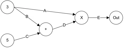
Figure 3.3 illustrates a simple, but complete, data ﬂow program consisting of two source

nodes, two intermediate nodes, and one sink node. In this example, assume the sink node

simply records the value of any tokens it receives for later review. Further assume the two

source nodes in this example are set to produce and send one token on each of their output

arcs. The produced tokens will contain a value equal to the label of their producing node. For

this example, arcsAandB will each carry one token of value3from the source actor labeled

“3”, and arcC will carry one token of value5. The two intermediate nodes “+” and “×” will

perform the operation described by their label, addition and multiplication respectively. During

execution, arcDwill carry one token of value8, produced by applying the addition operator to

tokens with values3from arcBplus5from arcC. Finally, the output of this program, carried

(24)

[image:24.612.189.424.69.160.2]

Figure 3.3: A simple data ﬂow program.

andOut=E.

The order of node execution in Figure 3.3 is easy and straightforward to determine. After

an actor’s data dependencies are met, that actor performs its assigned computation and the

result is propagated forward through the program. In data ﬂow programs, a node’s execution is

completely controlled by the availability of data, as carried by tokens, at its inputs. Therefore

such programs are referred to as “data-driven”.

Any token received at a node is stored by that node in an internal queue representing which

arc the token is received on. Once an intermediate node has received the required number of

tokens on each of its required input arcs, that node is considered “enabled”. Figure 3.4 (a)

shows a partially enabled node that has received a token on one of its two input arcs. Figure 3.4

(b) shows a node in its fully enabled state. After becoming fully enabled, an intermediate node

will autonomously “ﬁre”. When an actor ﬁres, it removes some tokens from its input queues,

performs some operation using the values of tokens it has received, and then produces one or

more tokens that are sent along the data ﬂow graph to the intermediate node’s successors, as

shown by 3.4 (c). Note that the token placed on the output arc is not the same as any of the

tokens consumed to produce it, although its value may be related (in this example a relation

by addition exists). The generalized data ﬂow model does not constrain the number of tokens

consumed or produced by an actor each time it ﬁres to be one, or even constant; a generalized

data ﬂow actor may produce or consume a varying number of tokens.

The above described process of actor ﬁring and token passing continues until some

termi-nation condition is met. During program execution an actor may receive and ﬁre many tokens.

A description of this model of computation has been formalized by Lee and

(25)

Figure 3.4: A partially enabled node (a), fully enabled node (b), and ﬁring node (c). A node is considered fully enabled if there is at least one token at each input arcs it requires to ﬁre.

tag pair, and a signal is deﬁned as set of such events. Using this deﬁnition, the output of a data

ﬂow program can be described from part, or all, of one or many of the signals generated during

the program execution.

Because data ﬂow programs allow an actor to ﬁre any time that input data is available, it is

possible for more than one actor to be ready for ﬁring at the same time. This offers the potential

for a high level of concurrency, often cited as a main advantage of data ﬂow programming

(Dennis, 1980, Lee and Messerschmitt, 1987). Unfortunately, because the data ﬂow model

lacks the concept of control ﬂow, program overhead must be spent to determine which actor

to ﬁre next when data ﬂow programs are run on computers lacking the appropriate hardware

architecture (Dennis, 1980).

Also important to the efﬁciency of a data ﬂow program is the granularity of that program’s

nodes. Complex operations can be built from a large number of simple units, or one complex

unit. The granularity of the model is considered course if the representative operations are

implemented as single, highly complex, actors or ﬁne granularity if the same operations are

represented as a collection of many, individually less complex actors. In a data ﬂow program,

larger granularity result in less overhead (Greening, 1988, Lee and Messerschmitt, 1987)

how-ever, due to their more abstract representation, models with courser granularity also contain

less structural information in their actor graphs.

Although not ideal from the standpoint of structural analysis, the reality that data ﬂow nodes

operate as independent processing units of any complexity greatly adds to the expressive power

of data ﬂow languages from the perspective of simulation modeling. Actors are not constrained

to implement only simple arithmetic operators, or even single expressions of many arithmetic

(26)

the authors show how it is possible to mix dataﬂow models with discrete-event models. One

example given by Chang et al. (1997) shows how a data ﬂow actor may itself implement a

dis-crete event simulation as its operation; instead of evaluating an expression of some parameters,

a data ﬂow actor could call a discrete event simulation and pass the result to other actors.

It should also be noted that actors may have internal state. An actor is allowed to remember

the values of any tokens it received, or any states derived from these tokens, since the start

of program execution. If the exact mechanics of a historically sensitive actor is known, it is

possible to convert it to an actor without state through adding a self-loop to communicate prior

state to itself between program iterations (Buck, 1993).

3.2.2

Petri Nets

Petri nets are a type of data ﬂow program commonly used for a variety of applications,

espe-cially the modeling of concurrent systems (Tadao, 1988). One speciﬁc example is the

applica-tion of Petri nets to manufacturing systems (Proth and Xie, 1996).

A Petri net is a directed bipartite graph containing nodes called places connected to nodes

called transitions (Proth and Xie, 1996). Transition nodes in a Petri net behave like actors, as

described above. Place nodes in a Petri net behave like relations as described above or, more

speciﬁcally, as a queue of tokens at an actor’s input.

Besides the differences mentioned above, Petri nets behave exactly as a simple form of

data ﬂow. Transitions are considered enabled when their dependencies are met (Proth and Xie,

1996). They then ﬁre or remove some tokens from their input places and put some tokens at

their output places. In basic Petri nets, these tokens are unlabeled. An important extension

to the Petri net model are colored Petri nets. Colored Petri nets use tokens having different

colors, or labels. They generally allow a more compact representation of a system, but are

disadvantageous in that many of the more useful analytical properties of elementary Petri nets

are not easily applied to colored Petri nets.

It is in the study of Petri Nets that many techniques for the study of synchronous data ﬂow

program structures originate. A review of such techniques, including examples which

(27)

tutorial of Petri nets’ usage in modeling, can be found in Tadao (1988).

3.2.3

Synchronous Data Flow

Synchronous data ﬂow (SDF) programming is a special case of data ﬂow programming where,

at least in its pure state, the number of tokens consumed and produced by an actor each time

it ﬁres is independent of the token values (Lee and Messerschmitt, 1987). This allows a static

order of execution for actors in a SDF program to be computed during the program’s

initializa-tion phase, greatly reducing some of the overhead associated with data ﬂow program execuinitializa-tion

(Lee and Messerschmitt, 1987). Furthermore, this assumption makes synchronous data ﬂow a

subclass of Petri Nets (Buck, 1993).

In reality, the synchronous data ﬂow language described by Lee and Messerschmitt (1987),

and which will be used to implement simulation models, differs from the above stated ideal.

The most notable difference is the inclusion of dynamic actors, two popular ones being the

switch and select actors shown in Figure 3.5, capable of producing or consuming a varying

number of tokens on each of their arcs (Buck, 1993). This extension of SDF can be made

with little impact to the scheduling and efﬁciency of the resulting programs, although some

scheduling decisions will need to be made at run time (Lee and Messerschmitt, 1987).

Figure 3.5: Two example dynamic data ﬂow actors.

The addition of dynamic actors to extend synchronous data ﬂow greatly improves the power

of such models. While basic Petri net models are not Turing-equivalent, dynamic data ﬂow

programs usually are (Buck, 1993).

An important property of the synchronous data ﬂow model of computation is that it contains

(28)

SDF model progresses globally to the model in discrete quantities referred to as “ticks” or

“iterations”, unlike discrete event and continuous time programs where time is modeled by the

application of a time-stamp to events.

Time is an important concept if a SDF program is to be used for certain simulation purposes.

One consequence of time dependent models is that an input factor may have an effect on a

model’s output instantly and to a constant extent over time, or that input’s effect may vary over

time- such an effect may be meaningless in the ﬁrst iterations but grow to be a dominate effect

after many. Such accumulations of effect may happen when state data is stored in an SDF

model between iterations, as happens when such a model contains a directed cycle.

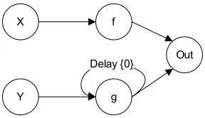
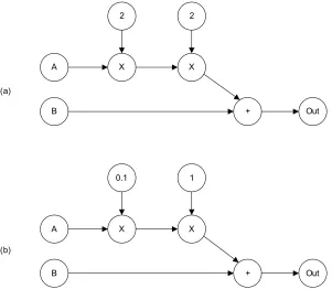
Figure 3.6 shows two actor graphs with a directed cycle between nodesAandB. The model

shown in Figure 3.6 (a) is impossible to start. NodeAdepends on both the value ofX and the

value ofBto ﬁre. NodeBdepends on nodeY and nodeA. Since nodeAdepends on nodeBand

nodeB depends on nodeA, a cyclic dependency exists which effectively prevents the model

from starting up. One way this cyclic dependency can be handled in SDF is to introduce a

delay on one of the arcs in the cycle (Lee and Messerschmitt, 1987). A delay holds any token

it encounters for some ﬁxed number of iterations before releasing it. Figure 3.6 (b) shows the

same model as (a) but with a single iteration delay on the directed arc fromAtoB. Since, by the

deﬁnition of synchronous data ﬂow, it must pass a token in every iteration, a delay must hold

an initial token at the beginning of execution for passage in the ﬁrst iteration. Curly brackets

are used here to show the initial token values contained by the delay, in this example one token

of value0. In the ﬁrst iteration of the SDF model from 3.6 (b), nodeB will take data from

Y and the delay, initially 0, to produce its output. In the Nth _{iteration, node}_B _{will take data}

fromY and the delayed output of A, or the value sent by A in iteration(N −1)to perform its operation. In a SDF model, it is required that all cycles be broken by a delay; failure to

do so is a structural fault that results in an unusable model (Lee and Messerschmitt, 1987).

Depending on the implementation language, delays may exist as attributes of the arc as shown

in this example or as specialized actor nodes on the network.

Cycles and delays in SDF can result in varying importance of an input over time, such as

(29)

[image:29.612.234.378.518.601.2]

Figure 3.6: An example SDF model with a directed cycle.

a state between iterations (although this can also be done internally by the actor). In the new

example of Figure 3.7, for example, assume the initial output of nodef isf(X) and nodeg’s output isg(Y,0). Note that nodeghas two input arcs, one of which is a self loop. Assuming X and Y remain constant, the values output in the second iteration forf and g aref(X) and g(Y, g(Y)), respectively. IfY were not constant, callY₀andY₁the initial and second iteration values ofY respectively, the value of g at the second iteration could be more thoroughly

de-scribed as g(Y₂, g(Y₁)). In general, the cycle around g in this example will cause g’s output on any given iteration to be partially dependent upon its output from the previous iteration,

which is itself partially dependent on nodeg’s output from the iteration before that. This

de-pendency continues recursively back to the ﬁrst iteration, with the result being that node g’s

output is dependent upon all historical values ofY. This recursive dependency is one deﬁnition

of a difference equation;x(n+ 1) =f(x(n))(Elaydi, 1996).

Figure 3.7: A SDF model with one self loop.

In this way, SDF programs may be used to simulate systems of difference equations; the

behavior of which can lead to highly dynamic behavior. There exist methods for ﬁnding exact

(30)

these solution methods to SDF programs would be extremely difﬁcult in practice, due in part

to the varying levels of granularity and transparency in SDF models. Although an actor may

contain a process to implement some functionf to map a set of inputsX to a set of responses

Y, no guarantee is made thatf itself is retrievable from the program. Any or all actors in a data

ﬂow program may be implemented as a “black-box“.

As with Petri Nets, since their structures are strongly graph based, synchronous data ﬂow

programs lend themselves well to graph theoretic based analysis. One simple example of this is

presented by Lee and Messerschmitt (1987) to verify the consistency of token production and

consumption.

Feng (2008) develops a model transformation approach to aid in the design of large

struc-turally conﬁgurable models. This is accomplished through the application of graph

transfor-mation algorithms. Principally concerned with the transfortransfor-mation of a model to speed up

con-struction and conﬁguration, Feng’s work is an example of how the graph structure of a data

ﬂow program can be examined and manipulated for productive purposes.

Of speciﬁc interest to analysis of a SDF simulation model is the ability to determine which

source actors, or inputs, have a causal impact on other actors in the model. A further question

is, given a set of source actors that have an effect on a given node, which of those effects are of

most importance.

The ﬁrst question, which inputs have an effect on which outputs, can be addressed using

“causality interfaces” (Zhou and Lee, 2008). A causality interface, as deﬁned by Zhou and

Lee (2008) states the dependency that an actor’s output signal has on input signals. It is also

shown that if the causality interfaces are known for all actors in an actor graph, it is possible

to determine the causality interface for the entire network, or composition of actors. Causality

interfaces are described by Zhou and Lee (2008) primarily as a means for deadlock analysis in

data ﬂow, or as a tool for discovering structural faults in a model.

Just having a causal effect does not necessarily indicate that effect has a meaningful

mag-nitude. Given a set of inputs that are known to contribute to an output’s value, the individual

effect of some inputs may be overwhelmed by the effect of others. The solution to this problem

(31)

even more difﬁcult with the existence of cycles, as was shown by example in 3.7. To date, there

does not appear to be any literature on ranking or identifying important effects using an actor

graph’s structure alone.

3.3

Review of Literature on Graph Structure Analysis

Considerable work has been done in developing methods to determine useful information from

structured data. Where graph based information exists there can often be found research into

how best to analyze that information. Some speciﬁcally interesting questions to the scope of

this thesis are:

• What makes a path of ﬂow through the graph important?

• What makes an individual node important, both globally and relative to another node?

This section contains a review of literature relevant to answering these questions, framed

by application to analysis of a data ﬂow program’s actor graph. Background information,

particularly on Markov chains, will be included as required.

3.3.1

Linear Signal Flow Graphs

Linear signal ﬂow graphs are a well established tool for studying and reducing complex

feed-back systems. They consist of a graph with nodes representing linear functions and arcs

rep-resenting the dependency of data between nodes. In this way, linear signal ﬂow graphs are

closely related to the data ﬂow programs described in Section 3.2.

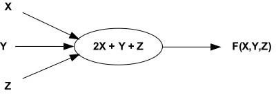
The behavior of a linear signal ﬂow graph can be described concisely by two rules. The

ﬁrst rule, shown by Figure 3.8 and described by X_i = n_j₌₁A_ijX_j, shows how values for individual nodes are computed (DeStefano, 1990).

The second rule, shown by Figure 3.9 andX_i =A_ikX_k, constraints values transmitted from a common source to be related by the value of the node which is their source (DeStefano, 1990).

Linear signal ﬂow graphs can provide a convenient graphical representation of linear

(32)

[image:32.612.253.359.64.191.2]

Figure 3.8: Addition rule for signal ﬂow graphs.

[image:32.612.253.362.229.357.2]

Figure 3.9: Transmission rule for signal ﬂow graphs.

a structural reduction is given by Figure 3.10 and its reduction, Figure 3.11.

Figure 3.10: Example linear signal ﬂow graph.

Figure 3.11: Reduction of example linear signal ﬂow graph.

This example shows how entire variables, and the nodes representing them, can be removed

by applying properties of multiplication. More complex examples of reduction, including

re-duction techniques that can simplify feedback loops, are given in DeStefano (1990).

Linear signal ﬂow graphs can be implemented as special types of data ﬂow programs,

how-ever the restriction that they contain only linear equations makes them, and methods for their

(33)

3.3.2

Path Importance

Paths on an actor graph represent channels over which information can ﬂow. In the context of

a data ﬂow actor graph, an important path may be considered one that is likely to have great

inﬂuence on an output of interest. This is to say, if information enters the head of an important

path, that information could be expected to prove very signiﬁcant to the information resulting

at the tail of that path.

A collection of paths connecting two nodes is a subgraph. In general, a subgraph is useful to

describe the relationship between two nodes when relationships between those nodes are

mul-tifaceted; often times representing a relationship using a single path is ineffective (Faloutsos,

Mccurley, and Tompkins, 2004). For an example in a social context, modiﬁed from an example

given by Faloutsos et al. (2004), imagine that your brother is married to your favorite author.

The shortest path between you and your sister in law on a social network would be that she is

your favorite author. It is, however, likely that your most important relation to her is through

her marriage to your brother. Multiple relationships like this exist in data ﬂow graphs. The

most important path between actors may not be the shortest, and many less important paths

may contribute to one most important effect. It is important to consider all paths between an

input and output of interest.

The concept of important paths are used heavily by the work of Mojtahedzadeh, Anderson,

and Richardson (2004), which discusses a method of analyzing a system dynamics model’s

structure called the “Pathway Participation Method” (PPM). The PPM starts with a single

vari-able (output) of interest, then works backward to determine the most important structure in the

model. This is accomplished by studying individual components to identify which path into

that component most inﬂuences the output. The PPM then recursively examines the

compo-nent upstream along the just identiﬁed path until the method converges on the most important

structure of the model.

Faloutsos et al. (2004) propose a method for discovery of important subgraphs connecting

two nodes. Their procedure treats the search for a subgraph as a maximum ﬂow problem. The

result is a collection of the important components comprising the potentially complex relation

(34)

3.3.3

Node Importance

The deﬁnition of node importance, as with the importance of a path, is ambiguous and domain

dependent. In literature, the interpretation of a node’s importance usually depends on the means

used to compute it.

It is easy to see how a measure for a node’s importance is useful in a variety of graph

structures. Considering the World Wide Web, one may be interested in the most important

website on the Internet. In social networks, the most important person in an organization may

be of interest. Analysis of a transportation system may be interested in the most important

bridge or intersection. In the actor graph of a data ﬂow program, it may be useful to determine

which actor is most important, the answer to which is synonymous with the most important

calculation. Although the meaning of an important node is interpreted differently in these four

examples (the Internet, social networks, transportation networks, and actor graphs), in each case

a node is considered important because it is somehow related to other nodes in a meaningful

way.

The importance of a node also depends on perspective. In a social network of a large

organization, the most important person on the whole graph is arguably the company’s leader.

Less globally, the most important person from the perspective of an individual in a company

is likely that individual’s immediate boss. A node’s absolute importance is deﬁned as the

importance of that node considering all other nodes in the graph. The relative importance of a

node can only be found speciﬁc to a subset of nodes.

Much work has been done on developing methods for discovering important nodes. Of

these methods there appear to be at least two main classes:

1. Methods that rank nodes based on graph theoretic notions (distance, node degree, etc.).

2. Methods that rank nodes by considering the graph to be a stochastic process.

3.3.3.1 Methods of Graph Theoretic Notions

Many methods from the ﬁrst class rely on measures of a node’s centrality in a graph.

(35)

transportation network, the highest degree node would represent the intersection with the most

roads entering it. In a data ﬂow actor graph, the highest degree node will represent the function

with the most input factors.

Global closeness is a method developed by Freeman (1979) to rank the centrality of a

node on a graph. Freeman deﬁnes a given node’s closeness centrality to be the sum of the

distance from that node to all other nodes on the graph. While closeness centrality is a useful

measure when distances on a graph hold important meaning, its power is limited when distances

themselves are not necessarily meaningful (Borgatti, 2005). Freeman (1979) also proposed

another measure of centrality called “betweenness”. Callg_ijthe total number of geodesic paths from nodeitojandg_ij(k)the number of those geodesic (shortest) paths passing through node k. The computation for betweenness centrality is then given by Freeman (1979) to be

i

j

g_ij(k)

g_ij ,∀i=j=k. (3.2) Essentially, betweenness centrality is a measure of how many geodesic paths pass through

nodek(Borgatti, 2005). As with global closeness, betweenness centrality is most relevant when

distance has meaning in a graph. Even so, measures of centrality in an actor graph may be

helpful in determining which nodes have the most widespread effect. If an actor on a data ﬂow

actor graph has a large inﬂuence on information passing through it, the larger that inﬂuential

node’s centrality measure, the more other nodes its inﬂuence is likely to effect.

3.3.3.2 Stochastic Process Methods

A second main class of methods for importance ranking is a class of methods which view a

given graph as a stochastic process. More speciﬁcally, assume a graph to be a representation

of a ﬁrst order Markov chain. A Markov chain is a discrete-time probabilistic model that is

useful for studying a system of states and transitions between those states. The study of a

Markov chain is facilitated by an application of the Markov assumption that the probability of

transitioning to any given state depends only on the current state of the system (Beichelt, 2006).

Under this assumption, a Markov chain can be completely described by a matrix of one-step

(36)

is in stateiat timen, it will transition to statejat timen+ 1with a probability ofp_ij. The system does not necessarily have to transition to a different state; it will remain in its current

state with probability p_ii. Being composed of transition probabilities, certain key properties must hold for the elements ofP:

0_≤p_ij ≤1,∀i,∀jand j

p_ij = 1,∀i. (3.3)

For representation as a Markov chain, the individual nodes of a graph should be considered

different states and arcs indicate transition probabilities between those states that may be

non-zero. Under this assumption, imagine a single token on the graph. If the token is at nodeiat

timen,Pfor this system is made up of some ﬁxed probabilitiesp_ijthat the token will transition to nodej. The token will only be allowed to transition between nodes if they are connected in

the graph;p_ij = 0if nodeiis not connected to nodej,1≥p_ij ≥0ifiis connected toj. If this single token is allowed to randomly transverse the graph (take a random walk), the long-term

fraction of time that this token is expected to be at any given node can then be thought of as an

estimate for that node’s importance (White and Smyth, 2003).

Further background in discrete-time Markov chains is required to fully understand the

me-chanics behind computing the long-term fraction of time a token is expected to reside at a

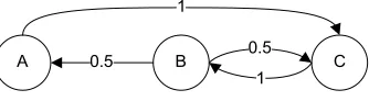
given state. Take for example the Markov chain described by Figure 3.12 which was built as

described above from the graph of Figure 3.13, assuming an equal probability of transition

along any outgoing arcs from a node. Because Node Bhas two out arcs, each arc has a0.5 probability of transition. IfNode Bhad three out arcs, each arc would be associated with a0.33 probability. The ﬁrst column and row ofPin Equation 3.4 refers toState A, the second column

and row to State B, and the third to State C. The 1 in the ﬁrst row and third column ofP in

Equation 3.4 refers to the 100% probability of transition fromState AtoState C. In this wayP

is closely related to the incident matrix of the graph from Figure 3.13.

IfPdenotes the single-step probabilities in a Markov chain,P2gives the two-step transition

probabilities, andPm is a matrix of them-step transition probabilities (Beichelt, 2006).

Ex-amples of the two-step, three-step, and hundred-step transition probabilities for the model of

(37)

P=

⎛

⎝00.5 0 00 1.5

0 1 0

⎞

[image:37.612.224.391.188.234.2]

⎠;p0 = (1,0,0)

Figure 3.12: Example Markov chain expressed as one-step transition probability matrix and initial probability vector.

Figure 3.13: Example Markov chain expressed as a graph.

What the individual matrices in Figure 3.14 describe are the probability of transition from

stateito state jin the number of steps indicated by the degree of P. The ﬁrst row of P3, for

example, shows that if starting inState 1, given three steps there is a0.5probability the system will end up back inState 1, and a0.5probability the system will end up inState 3.

The matrixP100seems to indicate that, regardless of the starting state, after100steps there is

a0.2probability of being inState 1, a0.4probability of being inState 2, and a0.4probability of being inState 3. In reality, the apparent indifference to starting state observed inP100of Figure

3.14 is due to rounding. If enough decimal places were displayed, it would be shown that,

given a start fromState 2, there is actually a slightly less than0.4probability of ending back inState 2after100steps. Even so,P100does suggest that the elements of the rows from these

m-step transition probability matrices are converging to some values asmapproaches inﬁnity, speciﬁcallyπ = (0.2,0.4,0.4). If a probability distribution vector that describes the long-term behavior regardless of the starting distribution vectorp0for the system under study exists, it is

called the stationary state probability vector and is referred to as the vectorπ(Beichelt, 2006). More formally, to be considered a system’s stationary state probability vector, the elements of

πmust satisfy a system of linear equations described by

π_j = i

π_ip_ij;∀j. (3.4)

(38)

P2 =

⎛

⎝ 00 01.5 00.5 0.5 0 0.5

⎞ ⎠

P3=

⎛

⎝00..25 05 0.5 00..255 0 0.5 0.5

⎞ ⎠

P100 =

⎛

⎝00..2 02 0..4 04 0..44 0.2 0.4 0.4

[image:38.612.246.362.76.251.2]

⎞ ⎠

Figure 3.14: Various m-step transition probability matrices.

3.4 andP0.

From this deﬁnition, the interpretation of π is synonymous with the long-term fraction of time that a randomly-walking token is expected to reside at any given node, one of the

importance metrics presented by White and Smyth (2003).

Variations on random walks for importance evaluation have been successfully applied to

a variety of applications. One successful example is the PageRank algorithm of Page, Brin,

Rajeev, and Terry (1999) used by the Google Internet search engine. The PageRank algorithm

has a strong foundation in random walks on graphs. A simplistic explanation of PageRank is

that a website is ranked highly if an individual randomly following links on a graph of the Web

is likely to spend a large percentage of his time at that given website.

Similar to the long-run proportion of time a random walker is expected to be at any given

node, measures of the token’s expected ﬁrst-passage time and commute time between nodes are

often cited measure of relative importance between nodes. The average ﬁrst-passage time of a

randomly walking token between two nodes is the expected number of steps that a

randomly-walking token, leaving the ﬁrst node, will take to reach the second (Fouss, Pirotte, Renders, and

Saerens, 2007). Expected commute time for two nodes is the expected number of steps required

for a round trip from the ﬁrst node to the second node and back to the ﬁrst. These metrics

can all be computed for a Markov chain, in a similar fashion to how the long-term residence

(39)

methods based on considering a graph to be a Markov chain work well when compared to other

standard scoring algorithms for a case study of a movie database; although they point out these

techniques are not likely to scale efﬁciently to very large systems. Even so, these methods that

view a graph as a stochastic process have the potential to be highly useful to analysis of a data

ﬂow graph, as they rely on the connection structure of a graph - not distances between nodes.

3.4

Discussion

Two hypotheses were proposed in the problem deﬁnition of Chapter 2. The ﬁrst stated

hypoth-esis, about the existence of information in a data ﬂow graph, has roots in prior work as detailed

in the review section on data ﬂow programming in Section 3.2 and the review of literature on

graph structure analysis in Section 3.3. Three speciﬁc examples on the analysis of a data ﬂow

program from that program’s structure were noted; one related to the use of model

transforma-tion to the constructransforma-tion of structurally conﬁgurable models, another related to consistency of

token production and consumption rates, and the third to deadlock, or liveliness, analysis.

More applicable to the goals of this thesis is the work of Mojtahedzadeh et al. (2004). In this

work, an analysis of a graph-based model is performed, called Pathway Participation Method

(PPM), to identify the most important paths through a simulation with respect to an output. The

PPM method, however, only considers the most important effect on individual components; it

does not account for instances where many paths in a model combine to result in large effects.

Furthermore, the PPM method focuses on identifying important model structures to aid in

model understanding, with less emphasis placed on the search for important input factors.

Taylor, Ford, and Ford (2007) proposes a method to utilizing the results from statistical

factor screening for the identiﬁcation of important model structures. After factors of high

im-portance have been identiﬁed, the model can be examined to see which model sub-structures

the most inﬂuential parameters are connected to; essentially the opposite of this thesis’s goal

of using important structures to identify important input factors. While of beneﬁt for model

A graph-based factor screening method for synchronous data flow simulation models

Rochester Institute of Technology

Recommended Citation

Contents

List of Figures

List of Tables

Acknowledgements

Chapter 1

Chapter 2

Chapter 3

Data Flow Programming

General Data Flow

Petri Nets

Synchronous Data Flow

Review of Literature on Graph Structure Analysis

Linear Signal Flow Graphs

Path Importance

Node Importance

Discussion