Evaluation of digital image compression algorithms for use on lap top computers

(1)

Rochester Institute of Technology

RIT Scholar Works

Theses

Thesis/Dissertation Collections

8-1992

Evaluation of digital image compression algorithms

for use on lap top computers

Bernard V. Brower

Follow this and additional works at:

http://scholarworks.rit.edu/theses

This Thesis is brought to you for free and open access by the Thesis/Dissertation Collections at RIT Scholar Works. It has been accepted for inclusion in Theses by an authorized administrator of RIT Scholar Works. For more information, please [email protected].

Recommended Citation

(2)

(3)

(4)

(5)

Evaluation

of

Digital

Image

Compression

Algorithms

for

Use

on

Lap Top

computers

by

Bernard V. Brower

Submitted to the Center for

Imaging

Science in partial fulfillment of the requirements for

the Master of Science degree at the Rochester Institute of

Technology

ABSTRACT

A technique for the evaluation of image compression algorithms was

developed. This technique was then applied in the evaluation of six

image compression algorithms

(ARIDPCM,

ISO/JPEG

DCT,

zonal

DCT,

proprietary wavelet, proprietary sub-band _coding and the _proprietary DCT). Of the six algorithms _evaluated, the Wavelet algorithm performed the best on average in image quality at all bit rates. The

JPEG DCT was concluded to be the most useful algorithm because of

its performance and the advantages that come with

being

an

(6)

ACKNOWLEDGEMENTS

The author would like to thank Dr. John R. Schott for his support, guidance and patience in this effort. The author would also like to express his appreciation for the technical advice given

by

his thesis committee: Dr. Roger

Easton,

Dr. Bob

Gray

and Dr Majid Rabbani.

The author would like to thank for their technical support Mr. Chris

Honsinger,

Mr.

Sterling

Mason and Mr. Bhavan Gandhi and the Eastman Kodak

Company

for

financial,

equipment, and materials support.

The author would like to acknowledge the

following

people and organizations who aided this _study

by

_submitting and _supporting proprietary image compression _algorithms;

Howard Resnikoff and John Huffman of Aware Incorporated.

Bahaa Fam from the Image

Processing

Research

Laboratory

of the MITRE Corporation.

(7)

Dedication

This thesis is dedicated to my parents, Ralph and

Monica,

whose moral and

(8)

Table of Contents

Table of Contents vi i

List of Figures xi

ListofTables xiii

1.0 Introduction 1

1.1

History

of study 1

1 .2 Digital Images 2

1.3 Motivation for Compression 2

1.3.1 Storage of Digital Images 3

1.3.2 Transmission of Digital Images 3

1 .4 Digital Image Compression 4

1 .4.1 Lossless Digital Image Compression 5

1.4.2

Lossy

Digital Image Compression 5

1.5 Evaluation of Compression Algorithms 5

1.6

Summary

6

2.0 Experimental Approach 8

2.1 Test Image Selection 8

2.2 BWC Algorithm Selection 9

2.3 Bit Rate 1 0

2.4 Algorithm Performance 1 0

2.4.1 Bit Rate

Accuracy

1 0

2.4.2 Image

Quality

Evaluation 11

2.4.2.1 Numerical Performance 1 1

2.4.2.2 Visual Performance 1 3

2.4.2.2.1 Test Image Set Selection 14

2.4.2.2.2 Evaluation Layout and Media 14

2.4.2.2.3 Evaluation Instructions 15

2.4.2.2.4

Rating

Scale 15

2.4.2.2.5

Rating

Sheet 16

2.4.2.2.6 Background Questionnaire 1 6

2.4.2.2.7 Evaluation Procedure 1 6

2.4.3

Complexity

and Speed of the Algorithm 1 7

2.4.4

Susceptibility

to Error 1 7

3.0 Compression Algorithm Description 1 8

3.1 ARIDPCM 1 8

3.1.1 Compression 1 9

3.1.1.1 Prediction and Error 19

(9)

Table of Contents

(cont.)

3.1.1.3

Coding

22

3.1.2 Decompression 22

3.2 ISO/JPEG Baseline Discrete Cosine Transform

(DCT)

24

3.2.1 Compression 24

3.2.1.1 Transform 26

3.2.1.2 Quantization 26

3.2.1.3

Coding

27

3.3 Zonal DCT 29

3.3.1.3

Coding

31

3.4

Proprietary

DCT 3 1

3.4.1 Compression 3 1

4.4.1.2 Quantization 3 2

3.4. 1.3

Coding

3 2

3.4.2 Decompression 3 3

3.5

Proprietary

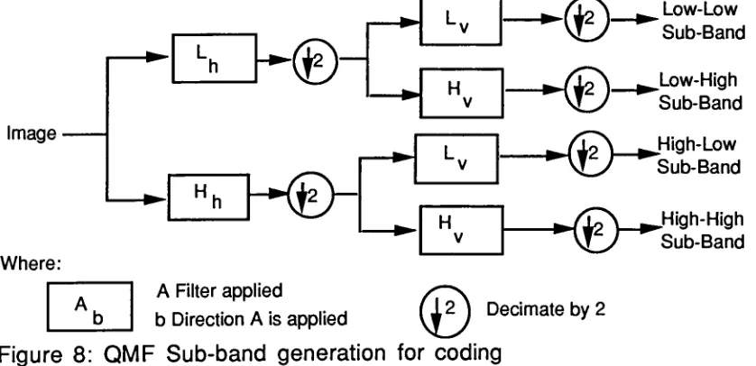
Quadrature Mirror Filter Pyramid Compression ...33

3.5.1.3

Coding

36

3.6

Proprietary

Wavelets Compression 37

3.6. 1 Compression 3 7

3.6.1.3

Coding

39

4.0 Results and Discussion 41

4.1 General Results 41

4.1.1 Bit Rate 41

4.1.2 Speedand

Complexity

42

4.1.3 Tolerance to Channel Error 42

4.1.4 Numerical Performance 43

4.1.5 Subjective Performance 45

4.2 Algorithm Results 47

(10)

Table of Contents

(cont.)

4.2.1.1 Bit Rate Control 47

4.2.1.2 Speed and

Complexity

48

4.2.1.3 Tolerance to Channel Error 48

4.2.1 .4 Objective Performance 48

4.2.1 .5 Subjective Performance 49

4.2.2 ISO/JPEG DCT 49

4.2.2.2 Speed and

Complexity

50

4.2.2.4 Objective Performance 51

4.2.2.5 Subjective Performance 5 1

4.2.3 Zonal DCT

(HVS)

52

4.2.3.2 Speed and

Complexity

52

4.2.3.5 Subjective Performance 53

4.2.4

Proprietary

DCT 5 3

4.2.4.2 Speed and

Complexity

54

4.2.5

Proprietary

QMF Pyramid Compression 55

4.2.5.2 Speed and

Complexity

55

4.2.5.5 Subjective Performance 56

4.2.6

Proprietary

Wavelets Pyramid Compression 56

4.2.6.2 Speed and

Complexity

57

4.3 Subjective Performance 5 8

4.3.1 Algorithm Performance Observations 58

4.3.2 Image

Quality

Observations 59

(11)

Table of Contents

(cont.)

References 68

Acronyms 70

Appendix A Evaluation Images A-₁

Appendix B Image Results Tables B-1

Appendix C Description of Evaluation Code C-1

Appendix D Description of SAS command Files for evaluation D-1

Appendix E Test Evaluation Packet E-1

Appendix F Example of

Rating

Sheet F-1

Appendix G Example of Exploitation Questions for the Images G-1

(12)

List of Figures

Figure _Title Page

1 Rate Distortion Curve for ARIDPCM on Test Image 4

2 Test

Transparency

Format 1 5

3

Rating

Scale 16

4 The levelsoftheARIDPCM 8-by-8 block 1 9

5 DCT Basis

Functions;

N =

8;

C = Coefficient Order 25

6 The

Zig-Zag

Format 2 8

7 Contrast

Sensitivity

Function 30

8 QMF Sub-band Generation for

Coding

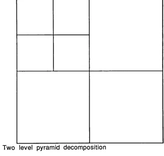
34

9 Two Level pyramid Decomposition 35

1 0 QMF Reconstruction Process 36

1 1 Daubechies Filter 3 8

1 2 Wavelet Sub-band Decomposition 38

13 Six level Pyramid Decomposition 39

1 4 Wavelet Reconstruction Process 40

15 Compression and Decompression Speed 42

16 Average RMS Error Performance vs. Bit Rate 43

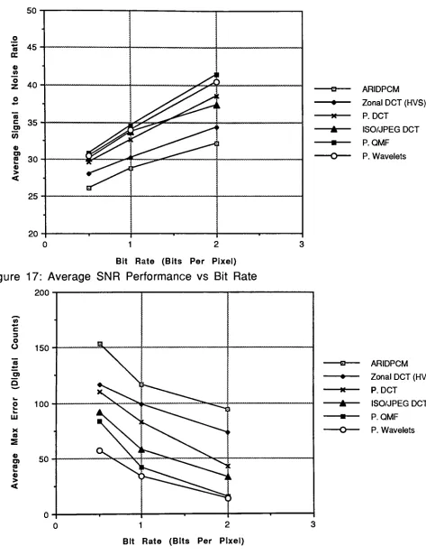
1 7 Average SNR Performance vs. Bit Rate 44

1 8 Average Maximum Error Performance vs. Bit Rate 44 1 9 Visual Image

Quality

at 2.0 bits per pixel 45 20 Visual Image

Quality

at 1.0 bits per pixel 46 21 Visual Image

Quality

at 0.5 bits per pixel 47

22 RMS Error Performance vs. Bit Rate for the ARIDPCM Algorithm 49

23 Normalization Factor Effect on Bit Rate 50

24 Average RMS Error Performance vs. Bit Rate for ISO/JPEG DCT 51 25 RMS Error Performance vs. Bit Rate for Zonal DCT 53 26 RMS Error Performance vs. Bit Rate for MITRE DCT 54 27 RMS Error Performance vs. Bit Rate for Sarnoff QMF 56 28 RMS Error Performance vs. Bit Rate for Aware Wavelets 58 29 RMS Error Performance vs. Bit Rate for Test Image 1 B-2 30 Max Error Performance vs. Bit Rate for Test Image 1 B-2 31 Signal to Noise Ratio vs. Bit Rate for Test Image 1 B-2 32 RMS Error Performance vs. Bit Rate for Test Image 2 B-4 33 Max Error Performance vs. Bit Rate for Test Image 2 B-4 34 Signal to Noise Ratio vs. Bit Rate for Test Image 2 B-4 35 RMS Error Performance vs. Bit Rate for Test Image 3 _B-6 36 Max Error Performance vs. Bit Rate for Test Image 3 _B-6 37 Signal to Noise Ratio vs. Bit Rate for Test Image 3 _B-6 3 8 RMS Error Performance vs. Bit Rate for Test Image 4 _B-8 39 Max Error Performance vs. Bit Rate for Test Image 4 B-8

(13)

List of Figures

(cont.)

Figure Title Page

41 RMS Error Performance vs. Bit Rate for Test Image 5 B-10

42 Max Error Performance vs. Bit Rate for Test Image 5 B-10

43 Signal to Noise Ratio vs. Bit Rate for Test Image 5 B-10

(14)

List of Tables

Title Page

BWC Test Images 9

Test Images Included in the

Engineering

Evaluation 1 4

ice Evaluation

Summary

4 1

Table

1 BWC T 2 Test In

3 Perforn 4 Numeri 5 Numeri 6 Numeri 7 Numeri 8 Numeri 9 Numer 10 Numeri 11 Numeri 12 Numer 13 Numer 14 Numer 15 Numer 16 Numer 17 Numer 18 Numer 19 Numer 20 Numer 21 Numer 22 Numer 23 Numer 24 Numer 25 Numeri 26 Numeri 27 Numer 28 Numeri 29 Numeri 30 Numer 31 Numer 32 Numer 33 Numeri 34 Numer 35 Numer 36 Numeri 37 Numer 38 Numer 39 Numeri ca ca ca ca ca ca ca ca ca ca ca ca ca ca ca ca ca ca ca ca ca ca ca ca ca ca ca ca ca ca ca ca ca ca ca ca Resu Resu Resu Resu Resu Resu Resu Resu Resu Resu Resu Resu Resu Resu Resu Resu Resu Resu Resu Resu Resu Resu Resu Resu Resu Resu Resu Resu Resu Resu Resu Resu Resu Resu Resu Resu Its fo Its fo Its fo Its fo Its fo Its fo Its fo Its fo Its fo Its fo Its fo Its fo Its fo Its fo Its fo Its fo Its fo Its fo Its fo Its fo Its fo Its fo Its fo Its fo Its fo Its fo Its fo Its fo Its fo Its fo Its fo Its fo Its fo Its fo Its fo Its fo

NITFS Test Image 1 at 0.5

bpp

B-3

bpp

B-3

bpp

B-3

bpp

B-5 NITFS Test Image 2 at 1.0

bpp

B-7

bpp

B-1 1

bpp

B-1 3 NITFS Test Image 6 at 1.0

bpp

B-23

bpp

B-23

bpp

B-25

bpp

B-25

(15)

List of Tables

(cont)

Table Title Page

40 Numerical Results for NITFS Test Image 13 at 0.5

bpp

B-27

bpp

B-27

bpp

B-27 43 Numerical Results for NITFS Test Image 14 at 0.5

bpp

B-29

bpp

B-29

bpp

B-29

bpp

B-31

bpp

B-31

bpp

B-31

bpp

B-3 3

bpp

B-33 51 Numerical Results for NITFS Test Image 16 at 2.0

bpp

B-33

bpp

B-35

bpp

B-35

(16)

1.0 Introduction.

It was once said that a picture is worth a thousand words. If this is taken

literally

then both sources of information should be the same size in bits

for digital computers.

Assuming

an average length of a word to be 4.5 letters and a half space on each end of a word (5.5

letters)

and _assuming an ASCII character (eight bits per _character), then 1000 words will

require 44,000 bits. This results in a

binary

image of about 210 pixels

by

210 lines which does not even equal the spatial

(approximately

640 pixels

by

460

lines)

or radiometric (8 bits per _pixel) resolution of television.

This exercise proves one of two things: either a picture is worth more

than a thousand words or images can be reduced in size with no loss of

information. In

truth,

both statements are correct. This thesis is

intended to evaluate the _capability of several digital image compression

algorithms for use on a personal computer. It also provides a consistent method _{for evaluating} compression algorithms.

1.1

History

of

Study

The National Image Transmission Format Standards

(NITFS)

is a _group of

Military

Standards that ensure

interoperability

between _secondary

imagery

users

(Army,

Navy,

Air

Force,

Coast

Guard,

Federal Bureau of

Investigation are some of the government agencies that are involved in the standards). The secondary

imagery

user is one that uses images in the

field (i.e. at diverse and often remote locations and _usually with little additional support _resources) and is most

likely

equipped with an AT-class Personal Computer (PC). This

family

of standards was developed

because different agencies within the Government could not _easily share

information in the form of images. Under the

funding

of the federal

government and the guidance of the NITFS Technical Board

(NTB)

this _study was completed to

help

the NTB select the next standard Bandwidth

Compression

(BWC)

algorithm for the NITFS. The original NITF BWC

standard was the Adaptive Recursive Interpolative Differential Pulse Code Modulation (ARIDPCM).(6) _This algorithm produced acceptable image

quality at 2.0 bits per pixel

(bpp)

with a reasonable amount of CPU time.

With the improvement of personal computers and BWC algorithms since

1984,

it was believed that there was an algorithm that could _{significantly}

(17)

1.2 Digital Images

Images will always be part of _society and

they

are ever _{evolving in} their

form. Original images started with drawings and paintings; the development of photographic film increased the _capability to record events

"exactly",

without artistic interpretation. Now digital images are

being

used everywhere from medical diagnosis to graphic arts to mass media.

Many

of the classical film-based systems

(X-rays,

hand held

cameras, . .

.) are converting to digital images because of the advantages

of digital images and of the associated equipment (e.g. speed,

flexibility,

range, . . . ). But along with the advantages of digital images come some drawbacks. One of the main problems is the _quantity of data associated with the digital images. For _example, _only one 512-by-512 24-bit color

image can be stored on a 1.44 megabyte 3.5 inch floppy. There is a need for compression of these images to maximize the _efficiency of storage and

transmission in real systems.

1.3 Motivation for Compression

Digital images have two main sources. The first type are direct digital sources which include some medical applications (e.g. CAT

Scan,

MRI and

digital

X-Rays),

digital cameras (e.g. Kodak's Hawkeye II and the Canon's

digital camera), computer-generated synthetic

images,

and remote

sensing satellites (e.g. SPOT and LANDSAT). The second source type is digitized analog data (e.g.

film,

video). These images can be monochrome,

single band (for most application of medical

images),

color (three

bands)

as in television and color photography, and multiple bands as in LANDSAT

(7

bands)

and MRI (3 Bands). Digital images come in many sizes.

Low-resolution images are most common in personal computer graphics

(

640 pixels per line and 480 lines per image with about 8 bits per pixel per band). Medium-resolution is used in _many photographic applications

(1024-by-1024,

8 bits per pixel per band). High-resolution images are

usually at least 2048

by

2048,

12 bits per pixel and are used for some

medical applications.

As digital images became popular, the increase in resolution resulted in larger files. A simple monochrome low-resolution image of 512 pixels

(18)

1.3.1 Storage of Digital Images

Storage of digital images is now _commonly used for medical records,

criminal records (both fingerprint and mug-shots), and with new digital

consumer products it will become more common to store personal

photographs

digitally

(Kodak Photo-CD). Another large database of images

is tax assessments of _{property for} the government. A small image

(512-by-512,

eight-bit _resolution), which is minimal

by

most standards, will

use about one-fifth of a double-sided

high-density

(1.44 _megabyte)

floppy

disk. A 40 megabyte hard drive will _{only hold} about 150 such

images,

which is not sufficient for storing images of all the buildings in a small

town or all the X-rays generated

by

a small hospital in a week.

By

compressing the images

8:1,

a 40 megabyte hard drive could store _up to

1,200 images.

1.3.2 Transmission of Digital Images

Transmission of digital images is

increasingly

_useful, e.g. for news/media

events. Newspaper images begin as lithographs of photographic images.

Then the lithographed image is transformed into a digital product which

can then be transmitted over a phone line. The best solution is the

transmission of the original digital images so that the local press can be

optimized for the original image. The transmission of a simple image

(512-by-512,

8-bpp)

over a common phone line at 2400 baud will take

approximately 11 minutes. With a compression rate of 2:1 this time is cut

in half and higher compression rates can decrease the transmission time

proportionally. The transmission of _{images is commonly} used in the

newspaper

industry

over phone lines and in the medical

industry

on

anything from phone lines to local area networks (e.g. ethernet ).

Another possibility is the use of radio transmission which _{is usually} of

lower quality

(noisier)

and has slower baud rates.

In these new scenarios a newspaper photographer could take the images

digitally,

review the images with the camera and find the nearest phone to

call the office to transmit the selected image.

By

_eliminating the

physical _{transportation,} photographic development and lithographic

processing the time it takes to get the picture back to the office is significantly reduced. A newspaper reporter can have the final shot of a

basketball game back to the main office before the fans have all left the

(19)

1.4 Digital Image Compression Basics

Most pictures, exhibit a large amount of data redundancy. For example, the sky in most images is quite uniform which means _{that any} given _sky pixel

is very similar to an adjacent _sky pixel. These pixels are

highly

correlated or have redundant information (similar

information)

in them.

Thus most digital images have high correlation between _neighboring

pixels. The average correlation of digital _{images is approximately} 90% for adjacent pixels.which translates to redundant information.

Compression algorithms

try

to reduce the redundant information _{in any} of

several ways. Digital image compression _{may be lossless (i.e. image is}

perfectly recoverable) or lossy. Lossless image compression will reduce

the redundant information with no loss of fidelity. In contrast,

lossy

digital image compression techniques always introduce some numerical loss of information. With a lossless image compression algorithm _only the algorithm itself has to be evaluated since the _{resulting images have}

not changed from the original. In

lossy

digital image compression the reconstructed _{image quality becomes} a major issue.

Many

of the

algorithms use the fact that the human vision system is less sensitive to certain spatial frequencies and certain noise patterns. This allows

greater compression of the digital images with no appearance of visual loss in the image. Lossless techniques are

typically

limited to

compression of about 2:1 to 3:1

depending

on the image and the

algorithm*4-5'8). The compression ratio for

lossy

techniques is limited

by

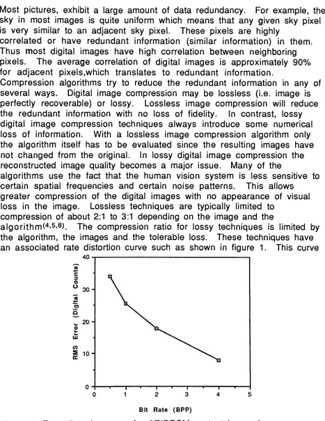
the algorithm, the images and the tolerable loss. These techniques have

an associated rate distortion curve such as shown in figure 1. This curve

40

0 1 2 3 4 5

[image:19.551.42.509.67.672.2]

Bit Rate _(BPP)

(20)

only accounts for numerical

distortion,

not visual distortion.

1.4.1 Lossless Compression

Lossless algorithms take advantage of local area correlation between

pixels and/or image statistics for compression. The most common

algorithm is Differential Pulse Code Modulation

(DPCM)

which uses a

weighted average of previous pixels (in either one-dimensional or

two)

to

predict the _gray value of the next pixel. _{The resulting difference between}

the actual and predicted pixel value is coded with a statistical coder (e.g.

Huffman encoder*4'5-8) _or _arithmetic coder*9-10)). Evaluation of lossless

algorithms is limited to speed of the _algorithm, _memory _{requirements,} and _{susceptibility} to channel error because image _quality is unchanged.

1.4.2

Lossy

Compression

Lossy

digital image compression techniques also use local correlation and

redundancy to reduce the number of _{bits necessary} to represent the image.

Ideally,

the _resulting _{image is visually identical (i.e. for} a given _viewing

condition), but can _{be visually lossy.} Most of the

lossy

algorithms can

compress the data

by

about 4:1 without significant visual loss. Increase

of the compression ratio results in more visual error. It is important to

understand how much error occurs with each algorithm and for what type

of image. Some algorithms perform better on a given type of image for a

variety of reasons:

1

)

some _may work better because

they

are tuned to a given image type;

2)

others _may work best because their innate artifacts are _relatively

undamaging to that data type.

1.5 Evaluation of Compression Algorithms

The performance of

lossy

algorithms are evaluated in four general areas.

First (and probably most

important),

is the _{image quality} at a given bit

rate. This provides one data point on a rate distortion curve shown in

figure 1. Other aspects (e.g. speed, susceptibility to channel _errors, rate

control) of the compression techniques _{may be} overlooked if the image

quality is superior for comparable bit rate. Most algorithms are compared

using this criteria alone but this is not sufficient for system design

which includes digital image compression as a component. In most

studies, the evaluation consists of comparison of rate distortion curves of

the given algorithm versus a general standard technique.*1-5-15'18) Other

(21)

compression technique in the context of the target system for which it is

being

developed. There are three main areas of compression use:

1)

storage of

data, 2)

transmission of

data,

and

3)

source system. The

storage of data is _usually internal storage either for long-term/archival storage or short-term storage. The main concern in these scenarios is the compression _speed, _{decompression} _speed, and the rate-distortion curve. The person _operating the system will not want to wait five minutes to decompress one image for display. In the transmission of the data another

obstacle is the noise in the transmission line. What are the artifacts caused

by

a bit error in the transmission line

(susceptibility

to channel errors). This is not a large concern in most scenarios because simple

error detection and correction

(EDAC)

codes can reduce the odds of a bit

error _affecting the image. The most concern is when _noisy channels are

used; the most common of these are radio

(UHF,

VHF)

communications channels. In source systems (e.g. _{hand-held digital camera) data-rate}

control is important so that real-time allocation to fixed storage space is

possible. The source system type is common in digital cameras and

remote _sensing systems where power, size and weight are a concern for the system design and packaging. Source systems algorithms will not be

specifically considered in this paper because of their

dependency

on

knowledge of associated hardware design. Another concern _{in selecting} a

compression algorithm is the

inter-operability

and public acceptance of

the algorithm (I.e. an algorithm which has wide acceptance will be more

functional to communicate with more people). The final concern in any

applications is the cost of the product. Although this will not be

specified in this report it is important to _many consumers.

1.6

Summary

One of the most _{important factors governing} the usage of digital images in

the world is digital image compression. People will always want better

quality (higher resolution)

images,

so as communication channels become

wider and storage _{memory becomes} cheaper people will want more data

(resolution). With this in mind there will always be a need for the

compression of the data. This is reflected in the commercial world

by

the

number of companies that are involved with digital image compression

(e.g.

IBM,

Eastman

Kodak, Aware, Optivision, C-Cube,

. . .). For some of

them, digital image compression products are the main source of income. This is also shown

by

the number of companies that are represented in the

American National Standards Institute

(ANSI)

and International

(22)

With the importance of compression there is a need to evaluate different

compression techniques for a given type of system. This thesis will

address one _way of _evaluating compression techniques. It will also evaluate six compression techniques on a _variety of images at multiple

(23)

2.0 Experimental Approach

With digital image compression

being

so common in the

literature,

there are _many established methods for evaluating the performance of an image compression algorithm.*3'4'5-8)

Many

_evaluations _consider

only the

compression rate and the image _quality at that given rate. Other factors may be important to properly design an

imaging

system. For example, an algorithm will not be used regardless of compression rate if the

processing time is excessive on a given computer system.

The

following

_study was developed for the purpose of _evaluating

lossy

compression algorithms for use in the Nation

Imagery

Transmission

Format Standards (NITFS). _{These military} standards define the

format,

communication protocols, compression techniques and other needs for the

interoperability

of digital image dissemination. This standard was defined for use with

Secondary

Image Dissemination Systems

(SIDS)

which are _{mostly based} on personal computers. _{The study} plan was developed to meet the needs of this standard. A wide _variety of images were selected for this _study and were compressed over a range of bit

rates

by

multiple image compression techniques. Then these

reconstructed images were evaluated with respect to numerical and visual accuracy and the algorithms were rated in speed/complexity, bit-rate accuracy and _{susceptibility} to channel error.

None of the algorithms were allowed to train on the test

images,

there

was a second set of images supplied for training.

The

following

subsections describe the _methodology and

history

of this

study. This description should allow the results to be replicated, at least in numerical performance.

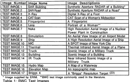
2.1 Test Image Collection

Seventeen test images were selected to represent the types of images

that might be exploited for information extraction

by

the users of NITFS. These monochrome

images,

each 512 pixels

by

512 lines

by

8 bits per

pixel, include high-resolution aerial

images,

medical

images,

digitized

maps, hand-held

images,

graphics, and images applicable to law

(24)

Image Number Image Name Image Descriptions

TEST IMAGE1 SAR Building Synthetic Aperture RADAR of a Buildinq*

TEST IMAGE2 SARRoad Synthetic Aperture RADAR of a Road*

TEST IMAGE 3 X-Ray Digital _X-Ray of a Foot

TESTIMAGE4 CAT Scan CAT Scanof aWoman's Midsection i TEST IMAGE 5 Fingerprint A Fingerprint

TEST IMAGE 6 Lena Portrait of a Woman**

TESTIMAGE7 Nuke High Resolution Aerial Image of a Nuclear Power Plant in Construction

TEST IMAGE 8 Simulation An Aerial View Image of an Airport Model TESTIMAGE9 _Ship A High Resolution Aerial Image of a_Ship

TEST IMAGE10 NYC ASPOT ImaqeofNew YorkCity

TEST IMAGE 11 Thermal Thermal Infrared Aerial Image of a Plane TEST IMAGE12 Truck Scenic Image of a _Military Truck

TESTIMAGE13 _Building Scenic Imageof a _Building

TEST IMAGE14 IR Truck Near Infrared Scenic Imageof a

Military Truck TEST IMAGE 15 Hydro Map AMapof aWaterway TEST IMAGE16 Elevation _Map Antopographic map TEST IMAGE17 Briggs 4 A "Briggs"

Resolution Target *23)

*

Image supplied _by ERIM. "BWC test image _commonly used in the literature.

Table 1 : BWC Test Images

2.2 Candidate Bandwidth Compression Algorithm Selection

The classical

lossy

image compression technique is a form of DPCM. A

compression algorithm in this class is the ARIDPCM. _{The simplicity} of

this algorithm has enabled its use on personal computers for years. But

the performance improvements of small _computers, _{their compilers,} and in the compression algorithms themselves have permitted the

consideration of hitherto complex algorithms. For example, the _relatively

recent development of the integer-based Discrete Cosine Transform

(DCT)

(as opposed to

floating-point)

has enabled the DCT to become practical on

IBM AT-class machines.

DCT is well known for producing excellent _{image quality} and is included in

the test matrix in three forms. The best known is the proposed ISO/JPEG DCT standard. The second of the DCT algorithms evaluated is the "generic"

zonal DCT algorithm. This algorithm is more complex than the ISO/JPEG algorithm, but has advantages in bit-rate control and in resistance to

channel error. The third DCT algorithm is a _proprietary algorithm submitted

by

the MITRE Corporation. This evaluation also included two proprietary forms of sub-band _coding compression

technology,

one

by

Aware Inc. and another

by

David Sarnoff Research Center. The sub-band [image:24.551.38.488.44.329.2]

(25)

2.3 Compression and Reconstruction

The test images were compressed to rates of

0.5, 1.0,

2.0 and 4.0

bpp

and then reconstructed. The three _{non-proprietary} algorithms were run

internally by

the author on a VAX-8700 and the _{images using} the three proprietary algorithms were processed

by

their respective companies. These bit rates were chosen to compensate for the

inherently

exponential

rate distortion curves over the bit rates of interest.

Sampling

in such a fashion minimizes interpolation errors for a fixed number of bit rates. An

example of a rate-distortion curve is shown in Figure 1. This study concentrated in the range of 2.0

bpp

to 0.5

bpp

because at 4.0

bpp

most algorithms were _{visually lossless.} _{The study did} not pursue higher

compression ratios because prior experience _{many images} are not useful

when compressed below 0.5

bpp

for these algorithms.

2.4 Algorithm Evaluation

The

following

sections outline the _methodology used in evaluating the test

algorithms for: bit-rate accuracy, image quality, susceptibility to channel error, speed, and complexity.

Only

software implementation techniques _using "standard" practices on serial computers were evaluated because of the cost of hardware

implementations. If hardware implementation had been considered then

additional evaluation techniques _{for complexity} would have been

necessary, such as physical _size, power consumption and absolute speed of calculations. Hardware implementations of interest would

include,

for example, small portable systems (hand held digital cameras) and remote

sensing systems.

2.4.1 Bit-Rate

Accuracy

Reliable control over the number of bits transmitted is important in

scenarios where transmission time or receiver storage is limited. To assess the performance of the algorithms in _{this area, the} algorithms are

first divided into two classes, driven and non-driven. A driven algorithm

produces a desired bit rate independent of the

image,

while a non-driven algorithm produces a bit rate that is dependent on both the image and the algorithm. The driven algorithms are then evaluated on the ease of

(26)

and the relative ease with which a non-driven algorithm can produce a

desired bit rate are reviewed.

2.4.2 Image

Quality

Evaluation

The most important part of the overall evaluation of a BWC algorithm is image quality. Bit-rate _accuracy, _speed, _complexity and tolerance to

channel errors are often compromised for higher image quality.

Image _quality loss is _generally divided into two classes, subjective and

objective. Subjective image _quality ratings rank the visual information loss of an image. _{Objective image quality} ratings yield information on the loss of the radiometric

(numerical)

information. Subjective observations

can differ from person to person

depending

on a _variety of factors such as the experience and age of the observer and _viewing conditions. Objective

ratings are unchanged from evaluation to evaluation. The problem with numerical performance is that it is not

directly

related to subjective image quality. This means that an algorithm _{may have} a larger numerical

error but appear to be better in visual image quality. This can happen if one algorithms exhibits greater error in areas or frequencies to which the

eye is _relatively insensitive.

2.4.2.1 Numerical Performance

The numerical performance values include root-mean-squared error

(RMSE),

signal-to-noise ratio

(SNR),

maximum _error, global _{image gray} level mean before and after compression, standard deviation before and

after _compression, and the _entropy of the original image and of the error images. These measurements were performed on each image at each bit

rate and for all the algorithms. It is important to note that

numerical performance values _may not be

directly

proportional

to subjective image quality.

RMSE is one of the most common objective _quality measurements used in

(27)

N

RMS Error =

\

^

=

VMSE

(1)

X(X'i-Xi)2

Where

Xj

is an original image _value,

X'j

is the reconstructed image and N is

the total number of pixels.

SNR is another common metric for evaluating BWC algorithms. SNR is

defined here as the ratio of the original image variance

(signal)

to the

mean squared error

(MSE)

of the compressed image (noise). The SNR is calculated

by implementing

Equation 2.

SNR =

10*Log10

Original Image Variance

MSE

(2)

An algorithm _may exhibit _relatively small global MSE while still

exhibiting objectionable error in isolated regions.

Generally,

a

computation of the maximum error will

flag

this effect. The Max error is

the maximum absolute value of the difference between the original and

the reconstructed image (Equation 3).

Max Error = MAX

(

ABS

(

X'

-X) )

(3)

Where X is the original image value and

X'

is the reconstructed image.

The overall statistics of the original and reconstructed images are

important if an automatic tone transfer curve

(TTC)

is used for display. A TTC remaps a given image to produce the "best" tonal _viewing conditions for a given image and monitor. A change in image statistics _may change the _resulting

TTC,

which will in turn change the appearance of the image.

In addition, a decrease in standard deviation _may also indicate increased

smoothing

by

the algorithm; conversely, an increase in standard deviation may indicate a noise increase. The mean and standard deviation of the images are calculated _{using Equations 4} and

5,

respectively.

N

iXi

Mean

(X)

=

(28)

N

X(Xj-

X)2

_

, i=1 Standard Deviation

(s)

=

\

rpj

(5)

where

Xj

is the value of the image at pixel

i,

X is the mean of that

image,

and N is the total number of pixels.

The final statistics to be calculated are the _entropy values of the original image and the error image. _{The entropy} of the original image

approximates the busyness of the original scene. _{The entropy} of the error image is intended to show the approximate bits per pixel _additionally

required to reproduce the original image without loss. _{The entropy} of an

image is calculated

from;

K

ENTROPY= _/Pi *

Log

i=1

1

P

(6)

where

Pj

_is _the _probability of _any given _gray value

(i)

in the image and K is

the number of possible _gray values (i).

2.4.2.2 Visual Performance

High-quality

images of the original and reconstructed images were

presented to a _group of people for evaluation. The evaluation images were 9 inches

by

9 inches photographic transparency. The production of these

images was optimized to produce the best images quality. Examples of

the original and reconstructed images are shown in Appendix A in smaller

and reflection print format. There were 34 evaluators _{ranging in}

experience from professional image analysts to engineers to _military

personnel. This evaluation was to determine the relative losses in visual utility due to the bandwidth compression

(BWC)

algorithms evaluated. Some areas of concern and points of interest of the images are presented

in section 5.4. This should enhance the readers'

ability to visually

(29)

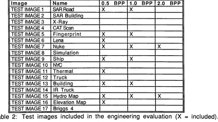
2.4.2.2.1 Test Image Set Selection

A subset of the 17 test images were chosen for visual evaluation (See Table 2). It was deemed unreasonable to evaluate all images at all bit

rates because of the amount of images to be viewed. The subset image set was chosen on the basis of image _{applicability} combined with

compressibility. For _example, Briggs targets and medical images were

eliminated; both of these image sets compressed _well, while the benefit

is questionable in comparison _{to aerial,}

hand-held,

or _{map images.} At 4.0 bits per pixel most images decompressed with the candidate BWC

algorithms produced _visually lossless results.

Therefore,

these images were eliminated from the test set. For the other

images,

preference was given to lower bit-rates. Decompressed images with negligible visual loss were eliminated from the test set.

Image Name 0.5 BPP 1.0 BPP 2.0 BPP

TEST IMAGE1 SARRoad X X

TEST IMAGE2 SAR _Building

TEST IMAGE 3 _X-Ray TEST IMAGE 4 CAT Scan

TESTIMAGE 5 Fingerprint X X

TEST IMAGE6 Lena X

TEST IMAGE7 Nuke X X X

TEST IMAGE8 Simulation

TEST IMAGE 9 Ship X X

TEST IMAGE10 NNC

TESTIMAGE 11 Thermal X

TESTIMAGE12 Truck

TEST IMAGE13 Building X X

TEST IMAGE 14 IR Truck

TESTIMAGE15 Hydro _Map X X X

TEST IMAGE16 Elevation Map X

[image:29.551.56.507.286.538.2]

TEST IMAGE 17 Briggs 4

Table 2: Test images included in the _engineering evaluation (X = included).

2.4.2.2.2 Evaluation Layout and Media

The six algorithms with the original data were rendered on positive nine-by-nine inch film transparencies. Transparencies present a wider dynamic

range and higher level of _consistency than can be rendered on prints. A light table was therefore required at each evaluation site. Figure 2

illustrates the format of a given test transparency. Each image within the

layout is 512 lines

by

512 pixels. The 1024-by-1024 images were

(30)

laser writer. These original negatives were contact printed to produce

multiple copies. _{Each copy} was checked for consistency. The upper left

image is the standard "original" against which all others were evaluated.

The remaining renditions for a given

image,

each _{corresponding} to a specific compression algorithm and a bit rate, were _randomly placed in

the _remaining three spots _among the transparencies.

Standard

Image

Algorithml

Rendition

Algorithm 2

Rendition

Algorithm

3

Rendition

Figure 2: Test

transparency

format

2.4.2.2.3 Evaluation Instructions

A set of instructions for performing the rating was supplied with each

test set. The instructions, shown in Appendix

E,

are a _step-by-step guide

through the test procedure. Because of the

diversity

of personnel and

differing

environmental conditions at each site, the instructions are _very

specific. While we assume the instructions were

followed,

the

evaluations were unsupervised. A set of instructions was sent with each

image set.

2.4.2.2.4

Rating

Scale

The evaluators were to rate each image on a _quality scale of +1 to -5 in

comparison to the original image (Standard). This scale could be

interpolated

by

the evaluator to an _arbitrary precision. Images were

evaluated in terms of exploitation loss of the compressed image as

compared to the original uncompressed image. Each algorithm was

evaluated in comparison _{only to the} original image standard; no _scoring

should have been based on comparison between two or more algorithms.

(31)

+1

-3

-5

Slight improvement compared to the standard No noticeable difference from the standard

Slight change in the imagecompared to standardbut no loss in utility Slight loss in utility compared _{to standard,} but adequate to perform exploitation

Significant _{loss in utility} compared to standard (adequate to perform exploitation but _{may seriously} affect accuracy of _{exploitation)}

Excessive utility loss compared to standard (unusable for exploitation but usable for briefings and orientation)

Excessive utility loss compared to standard (unusable for any purpose)

Figure 3:

Rating

scale

2.4.2.2.5

Rating

Sheet

A rating sheet example is shown in Appendix F. Possible exploitation

questions/tasks, based on the image at

hand,

were provided for each image. Appendix G shows sample questions for test image

7,

an aerial view of the construction site for a nuclear power plant.

2.4.2.2.6 Background Questionnaire

A personal data sheet, shown in Appendix

H,

was completed

by

each evaluator and was intended to categorize the image exploitation

experience of each evaluator if statistical _weighting would have been required.

2.4.2.2.7 Evaluation Procedure

The data were screened for outliers

by

_using standard statistical techniques. Flagged outliers would have been considered for removal according to such factors as individual experience with the given data type. No outliers were discovered.

An analysis of variance

(ANOVA)

table was used to interpret the results. The ANOVA table allows

testing

for

biases,

which might be due to the

expertise of the evaluator on an image type, the image data or the bit-rate. Each bit-rate was considered _{separately because}

they

are discrete points on the rate-distortion curve. The ANOVA _{table produces,} in this

case, a mean visual _{rating, the} variance of the _rating and a prediction of

(32)

same significance group. A single algorithm can be placed in two

different significance groups which implies that _group one is

significantly different from group two but that the algorithm is not

significantly different from either of the groups.

2.4.3 Algorithm

Complexity

and Speed

The complexity and speed of a BWC algorithm are important to small

computer users. For this _study each algorithm was evaluated on the basis

of the number and type of operations

(multiplies,

divides, look-ups,

_etc.)

performed per pixel. These numbers translate to approximate _running

time for a computer platform benchmarked for the speed of each operation

assuming a serial implementation of the algorithm.

Relative running times for each algorithm on a given machine are

presented for both compression and decompression. While the relative

algorithm performance is accurate for the configurations _presented, the

actual times will _vary

depending

on specific implementations. A general

goal of the NITFS is to compress and decompress a 512-by-512 sample

image in less than two minutes each direction.

2.4.4

Susceptibility

to Error

Channel bit-error effects are important for evaluating BWC algorithms

used in transmission. Some algorithms will suffer localized information

loss from a bit error, while others _may experience total image

destruction.*4) _This indicates certain algorithms _may have different error

detection and correction requirements. Error detection algorithms reduce

the loss of information in an image but also increase _{the overhead,} which

in turn increases the total bit rate. The effects of bit errors

during

(33)

3.0 Compression Algorithm Description

Spatial compression can be performed on images only if neighboring pixels

are correlated. In _{general, the} higher the correlation between _neighboring

pixels the more compression that can be achieved. Most

lossy

spatial

compression algorithms work in three phases: _prediction, quantization and

coding. The first is the transform or prediction or "representation" or

"model"

phase, which takes advantage of the correlation between pixels.

This phase, which is usually

lossless,

decorrelates the data

by

either

transform or prediction methods. The intent of the transform or

prediction is to minimize the redundant information in the image.

The second phase of the compression process is the quantization of the

data. Losses in image

fidelity

are

directly

attributable to this step.

However,

the amount of loss is a function of both the transform/

prediction method and the quantization _strategy employed. Examples of

common quantization strategies are Lloyd-Max quantization and Pulse

Code Modulation (PCM).*4)

The quantized values are coded in the third and last phase. The two _coding

methods discussed in this _study are a fixed-length

binary

code and a

variable-length coder. Constant-length

binary

codes with n bits per pixel

can store 2n values. These values are representative of integer values

between 0 and

2n-1,

or of values that are hard-coded in a

look-up

table.

In variable-length _coders, the length of the code is a function of the

probability of occurrence of a given data point. An entropy coder is the

most common variable-length coder. Other examples of _coding strategies

are the Mel-coder and the Lempel-Ziv*4) technique.

In sections

3.4,

3.5 and

3.6,

_only a limited discussion of the algorithms

can be presented due to their _proprietary nature. More information can be

obtained from the references given and the companies that have submitted

the algorithms.

3.1 ARIDPCM(3.6)

The ARIDPCM algorithm consist of _partitioning the original image into

8-by-8 pixel neighborhoods, generating hierarchical prediction matrices for

those neighborhoods, and then _quantizing the difference images (original

-predicted) at each level of the hierarchy. As outlined in the NITFS

(34)

mode.

Only

the driven mode will be discussed since it ensures a fixed compression rate.

3.1.1 Compression

The driven mode is a two-pass algorithm. The first pass generates the prediction _matrices, finds the difference images and then classifies each difference neighborhood in terms of its activity. The second pass

quantizes the delta pixel values (from the difference

image)

in each neighborhood _according to _{its activity} classification. As in

DPCM,

compression is achieved through _quantizing the difference image with fewer bits.

3.1.1.1 Prediction and Error

Each image is subdivided into 8-by-8 pixel neighborhoods

beginning

at the upper left corner of the image. All of the prediction are made with the original values. Each neighborhood is comprised of

levels;

one Level-1 pixel

(L1),

three Level-2 pixels

(L2),

twelve Level-3 pixels

(L3),

and forty-eight Level-4 pixels

(L4)

(see figure 4 for Level map).

EI

L3 L3 L4 L4 L4 L4 L4 L4 L4

Inn*

L3 L4 L3 L4 L3 L4 L3 L4 L3 msasm L4 L4 L4 L4 L4 L4 L4 L4 L2 mimai L4 L3 L4 L4 L4 L3 L4 L4 L4 L4 L4 L4 L4 L4 L3 L4 L3 L4 L3 L4 !L3 L4 L3 L1 L4 L4 L4 L4 L4 L4 L4 L4 L3 L4 L4 L3 L4 L4

lL1

(35)

The notation used to describe the neighborhood matrices is

Di.j

=

Uj

-pij;

difference matrix.

Li.j

= Actual _pixel _value _at Pixel _i,j.

Pi.j

= Predicted pixel value at Pixel i,j.

The sub-image blocks are referenced in the bottom right corner (i =

j

=

0),

with

i,

j increasing

from right-to-left and

bottom-to-top

respectively.

A prediction matrix is computed for each neighborhood

by

_using an

additional column to the left and an additional row to the

top

of the

neighborhood. In total, a 9-by-9 sub-image block encompassing the

neighborhood of interest is required to create its prediction matrix. If the

neighborhood of interest borders the

top

or left edge of the

image,

an

artificial 9th row and/or column is created

by

_copying the first row or

column in the neighborhood respectively, and

Ls,8

is assigned Lrj,0- The

following

linear and bilinear interpolation scheme is used to compute the prediction matrix for each neighborhood.

Level 2 pixels:

Po,4

=

(

L0,o

₊

Lo,8

)

/ 2

(7)

P4,o

= (L0,o+ L8>0)/2

(8)

P4,4

=

(

L0,o

₊

L0,8

+

1-8,0

+

L8i8

)

/ 4

(9)

Level 3 pixels:

Pij

=

(

LU-2

₊

Lu+2 )

/ 2 for i-

0,

4 _and j.

2,

6

(10)

Pij

-

(

Lj.2ij

+

Li+2ij

)

/ 2 for i.

2,

6 and j-

0,

4

(11)

Pi.j

=

(

Lj-2,j-2

+

U-2.J+2

+

Li+2,j-2+

Li+2>j+2)

/ 4 for i=

2,

₆ and j=

2,

6

(12)

Level 4 pixels:

Pij

=

(

Li.j.1

+

Li>j+i

)

/ 2 for i=

0, 2, 4,

6 and j-

1, 3, 5,

7

(13)

Pij

=

(

Lj.-ij

+

Li+i,j

)

/ 2 for i=

1, 3, 5,

7 and j=

0, 2, 4,

6

(14)

Pij

=

(

U-ij-i

₊

Li-i,j+i

+

Li+i,j-i

+

Li+1fj+i)

/ 4 for i=

1, 3, 5,

7 and j=

1, 3, 5,

7

(15)

The difference matrix or error _{map is} computed

by

set:

DiJ

=

U.j

-

Pij.

(36)

This, however,

does not include the corner point which is a Level-1 pixel.

Do,o

=

L00.

(17)

The level-1 delta pixels are assigned their original pixel values.

3.1.1.2 Quantization

Each difference neighborhood is classified in terms of its activity. A

measure of _{activity is}

"Busyness",

which is defined as the maximum

difference of the Level-4 delta pixels.

Busyness =

Max(D4)

-Min(D4)

(18)

Each difference neighborhood is classified as either an

A,

B, C,

or D

Busyness;

D

being

the busiest.

In the driven mode of _operation, the first pass computes the _activity of a

neighborhood. Thresholds for each busyness class are then computed such

that a fixed percentage of the neighborhoods falls into each classification.

This guarantees data compression at a specified fixed rate. Table 8 in

NITFS document Version 1.1 shows the percent Busyness classification for

a selected bit rate.

The quantization of the difference pixel is done with the use of

hard-coded

look-up

quantization tables that are dependent on the busyness

class, level of the pixel and the difference value of that pixel. The

Level-1 pixels are always quantized to their full image resolution (8 bits).

Standard quantization tables were derived

by

_using Level-4 deltas from

sample images. The population distribution of the Level-4 deltas was

determined and divided into N continuous regions of equal population (N =

2",

were n represents the number of bits allocated for a given level in the

BAMs). The hard-coded Bit Allocation Matrices

(BAM)

and quantization

(37)

3.1.1.3

Coding

The quantized levels are coded with a constant-length

binary

look-up

table code. The number of bits in the

BAM,

the compression _rate, and the

quantized value are used as indices to the

look-up

table.

3.1.2 Decompression

The image decompression process is the reverse process of the

compression scheme. The received data is used to reconstruct the

predicted _matrix, which in turn allows reconstruction of the image. The

notation used to describe this process is:

E[

Djj

]

= Estimated _value _of

Djj

after dequantization.

Ri,j

=

E[Dij]

+

P|j.

Rjj

= Reconstructed value at pixel i,j.

Pij

= Predicted _value _at _pixel i,j.

Ljj

= Actual _value _at pixel i,j.

The

(R0,o. Ro,8, Rs.o,

Rs.s)

pixels are equal to

(L0,o> L0,8, U.o,

L8>8)

pixels

since Level 1 pixels are transmitted in full 8-bit resolution. The

remaining image values are reconstructed

by

_{consecutively computing} the predicted values and their _{corresponding} reconstructed values.

Level-2 pixels:

The predicted values for level-2 pixels are

Po,4

=

(

Ro.o

+

Ro,8

)/2

(19)

P4,o

=

(

Ro.o

₊

Rs.o

)/2

(20)

P4.4

=

(

Ro.o

₊

Ro.s

₊

Rs.o

+

Rs.s

)/4. (21

)

The corresponding level-2 pixel values are reconstructed _using

R0,4

=

E[

D0)4

]+

Po,4

(22)

R4,o

= E[D4,o]+

P4,o

(23)

R4l4

=

E[

D4,4

]

₊

P4.4.

(38)

Level-3 pixels:

From these reconstructed values _{already derived} and _using the

reconstructed values for

(

R4.8,

Rs,4 ),

P4.8

=

(

Ro,8

₊

R8,8

)/2

P8,4

= (R8>0+ R8,8)/2

(25)

R4,8

=

E[

D4,8

]+

P0,4

(26)

R8,4

=

E[

D8i4

]+

P8>4

(27)

the

following

Level-3 predictions can be made.

=

( Ri,j-2

₊

Ri,j+2

)/2 for i=

0, 4,

8 _and j=

2,

6

(28)

=

(

Ri-2,j

+

Ri+2,j

)/2 for i=

2,

6 and j=

0, 4,

8

(29)

=

( Ri-2,j-2

₊

Ri-2,j+2

₊

Ri+2,j-2

+

Ri+2,j+2

)/4. for i=

2,

6 and j=

2,

6

(30)

The corresponding reconstructed values are then computed _using

Ri.j=

E[

DU

]

+

Pij.

(31)

Level-4 pixels:

The level-4 predicted values are made _using the above reconstructed

values.

Pij

=

( Rjj.1

+

Ri,j+1

)/2 for i=

0, 2, 4,

6 and j=

1, 3, 5,

7

(32)

Pij

=

(

Ri'ij

+

Rmj

)/2 for i=

1, 3, 5,

7 and j=

0,

2, 4,

6

(33)

Pij

=

(

Ri-ij-i

+

Ri-ij+i

+

Ri+ij-i

+

Ri+i,j+i

)/4 for i=

1,

3, 5,

7 and j=

1, 3, 5,

7

(34)

The remaining reconstructed values are computed

by

_using

Rlj

=

E[

Dy

]

+

Pij.

(35)

This completes the reconstruction process for all pixel values within an 8-by-8 neighborhood. This process is repeated until all neighborhoods are

(39)

3.2 ISO/JPEG Baseline Discrete Cosine TransformC,3,4,5,6,7,8)

The ISO/JPEG baseline DCT is a sequential 8-bit DCT with Huffman

encoding. This DCT is a one-pass algorithm comprised of a 2-D 8-by-8 DCT transform followed

by

separate Huffman encoding of the set of DC

coefficients; the AC coefficients are encoded with Huffman codes and run

lengths. The improvement _{in quality} compared to the standard Chen-Pratt

(threshold)

DCTO) is in the quantization of the DCT coefficients. The

ISO/JPEG DCT has been implemented in a

fast, integer-based,

transform

which increases the speed of the transform with minimal quantization

errors. This implementation of the DCT has made its use in a PC-based

system more amenable.

3.2.1 Compression

The correlation structure for most realistic gray-scale images is

approximately Markov in character. When the equations _governing the

Karhunen-Loeve

(KL)

transform are applied to a first-order Markov process

with high spatial _correlation, the _resulting transform _{looks very} much

like the transform of a DCT. The DCT is thus assumed to _{be nearly}

optimum for a block transform of a given size, as a _{variance-compacting}

decorrelator with respect to imagery.

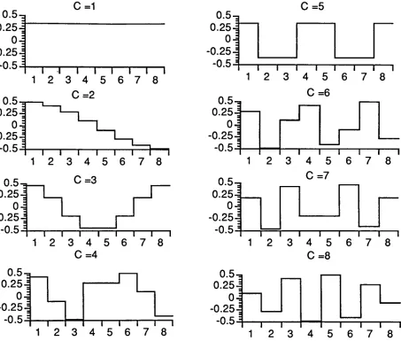
The DCT _{is significantly faster} than a spatial KL transform. Figure 5

shows the DCT basis functions for a block size of 8. The transform

coefficients _{corresponding} to each of the basis functions measures the

similarity of the pixels in the block and the _{corresponding} basis functions.

The sign of the coefficients indicates negative or positive correlation

with the basis function.

The 1-D basis function are represented in two dimensions

by

equation 36.

The 1-D functions can be applyed in the lines direction and then the

samples direction because of their separability. This can increase both

(40)

0.5-g

0.25-j 04

-0.254

-0.5-i

C=1

0.5-=

~l 1 I I I I I I

12 3 4 5 6 7 8

C=2

0.5, C=3

1 I 1 T I 1 1 1

12 3 4 5 6 7 8

C=4

0.5-=, 0.254

04

-0.25-1

-0.5^

n

i i i i i

1 2 3 4 5 6 7 8

0.5-= 0.254 0-j

-0.25-j

-0.5-:

C=5

0.5-g

0.254

04

-0.254

-0.5-S

I I I l I I I

12 3 4 5 6 7 8

C=6

0.5-a 0.254

0-1

-0.254

-0.5-^

\ 1 1 1 1 1

1 2 3 4 5 6 7 8

C=7

I I 1 1 1 1 1 1

12 3 4 5 6 7 8

C=8

O.5-3

0.254

04

-0.254

-0.5i

1_

I 1 1 I 1 1 1 1

[image:40.551.53.506.50.435.2]

1 2 3 4 5 6 7 8

(41)

3.2.1.1 Transform

The ISO/JPEG DCT process first divides the image into 8-by-8 blocks. The

8-by-8 DCT of each block is computed. The transform equation is:

(4C(u)C(v))n-1n-1 _(2j ₊ _1)up ₍₂_k ₊ _1)vp F(u,v) = A

'2K _''

1

f(J.k)cos(* _2/ P)cos(A ^T^

(36)

n j=o k=0

where

F(u,v)

is the DCT value for the point _u, v in the 8-by-8

block,

f(j,k)

is the original image value for the pixel

j,

k of the 8-by-8

block,

and

C(w)

= . for w ₌ 0

and

C(w)

=1 for w =

1,2,3,

. . . _, N-1.

For most images the _{energy is} concentrated in the low spatial frequencies

(upper left corner). The extreme upper left value is the DC value

(i.e.,

zero

frequency)

which is proportional to the mean of that block. The other

values increase in

frequency

and _{generally decrease in energy from} the

upper left to the lower right.

3.2.1.2 Quantization

The ISO/JPEG DCT quantization tables have been adapted to reflect the

sensitivity of the human visual system (HVS).*8'21) This HVS quantization

is optimized to reduce information without _sacrificing perceived image

context. The benefits of HVS quantization can be thought in two ways:

1. The same visual _quality can be obtained with less data (i.e. more

compression).

2. Improved _{image quality} can be obtained with the same _quantity of

data.

Quantization is performed

by

dividing

the transform data

by

a factor for

that

frequency

and _quantizing to a nearest integer. Compression is

increased

by

_multiplying the quantization table below (annex of the JPEG

(42)

16

(DC)

1 1 10 16 24 40 51 61

12 12 14 19 26 58 60 55

14 13 16 24 40 57 69 56

14 17 22 29 51 87 80 62

18 22 37 56 68 109 103 77

24 35 55 64 81 104 113 92

49 64 78 87 103 121 120 101

72 92 95 98 112 100 103 99

The error associated with compression occurs at this step. This is an

example, and _may not be suitable for normal _viewing conditions because of the lack of symmetry.

3.2.1.3

Coding

The DC coefficient is extracted from the 8-by-8 block and coded

separately. The DC coefficient of the adjacent block is used as a predictor

and the difference is Huffman encoded. _{The remaining 2-D array} of

quantized AC coefficients are placed in a 1-D _array

by

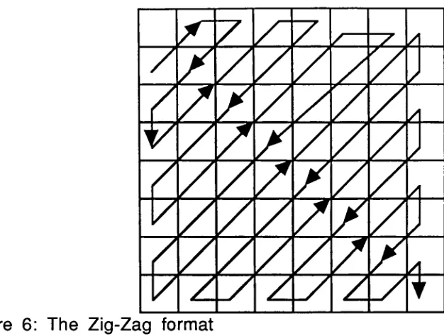
_zig-zag _ordering, shown in Figure 6. This reformats the transform coefficients into

approximately

decreasing

order of expected _energy and allows them to be run length encoded. The AC coefficients are Huffman encoded with

additions to the code for runs of zero coefficient and end-of-block

(EOB)

data. The EOB is used at the last non-zero AC coefficient. This reduces

the number of coefficients to be coded since most of the high

frequency

values tend to be zero, especially after the HVS quantization. The Huffman and quantization

(normalization)

tables can be optimized for a

(43)

[image:43.551.73.386.47.284.2]

Figure 6: The

Zig-Zag

format

3.2.2 Decompression

The ISO/JPEG DCT decompression process is a mirror image of the

compression process. The decompression process consists of four stages:

1.

decoding

the Huffman code

2. recreate the 2-D block

3. dequantization

4. inverse DCT.

The transform from discrete cosine domain to image domain is executed

using Equation 37:

(4C(u)C(v)) n-1 n-1

(2j

+ _1)up (2k + _1)vp

,v f(j,k) = [

4

I F(u,v)cos(^ ' >os(j ^Ji)

(37)

n u=o v=0

2n

where

F(u,v)

is the DCT value for the point _u, v in the 8-by-8 block

f(j,k)

is the reconstructed image value for the pixel

j,

k of the 8-by-8

block,

and

C(w)

=

-?=-for w = 0 _and

C(w)

= 1 for w = 1,2,3 N-1.

V

2

Again,

equation 37 is the definition of the

floating

point inverse DCT