Simple framework for real time forecast in a data limited situation: the Zika virus (ZIKV) outbreaks in Brazil from 2015 to 2016 as an example

RESEARCH

Simple framework for real-time forecast

in a data-limited situation: the Zika virus

(ZIKV) outbreaks in Brazil from 2015 to 2016

as an example

Shi Zhao

_{, Salihu S. Musa}

_{, Hao Fu}

_{, Daihai He}

_{and Jing Qin}

Abstract

Background: In 2015–2016, Zika virus (ZIKV) caused serious epidemics in Brazil. The key epidemiological parameters and spatial heterogeneity of ZIKV epidemics in different states in Brazil remain unclear. Early prediction of the final epidemic (or outbreak) size for ZIKV outbreaks is crucial for public health decision-making and mitigation planning. We investigated the spatial heterogeneity in the epidemiological features of ZIKV across eight different Brazilian states by using simple non-linear growth models.

Results: We fitted three different models to the weekly reported ZIKV cases in eight different states and obtained an R2 _{larger than 0.995. The estimated average values of basic reproduction numbers from different states varied from} 2.07 to 3.41, with a mean of 2.77. The estimated turning points of the epidemics also varied across different states. The estimation of turning points nevertheless is stable and real-time. The forecast of the final epidemic size (attack rate) is reasonably accurate, shortly after the turning point. The knowledge of the epidemic turning point is crucial for accurate real-time projection of the outbreak.

Conclusions: Our simple models fitted the epidemic reasonably well and thus revealed the spatial heterogeneity in the epidemiological features across Brazilian states. The knowledge of the epidemic turning point is crucial for real-time projection of the outbreak size. Our real-real-time estimation framework is able to yield a reliable prediction of the final epidemic size.

Keywords: Zika virus, Brazil, Modeling analysis, Reproduction number, Epidemic size, Spatial heterogeneity

© The Author(s) 2019. This article is distributed under the terms of the Creative Commons Attribution 4.0 International License (http://creat iveco mmons .org/licen ses/by/4.0/), which permits unrestricted use, distribution, and reproduction in any medium, provided you give appropriate credit to the original author(s) and the source, provide a link to the Creative Commons license, and indicate if changes were made. The Creative Commons Public Domain Dedication waiver (http://creat iveco mmons .org/ publi cdoma in/zero/1.0/) applies to the data made available in this article, unless otherwise stated.

Background

Zika virus (ZIKV) was first identified in the Zika For-est of Uganda in 1947 [1]. Later it was found to spread in the human populations in Nigeria [2, 3]. ZIKV is an arbovirus in the family of Flaviviridae and is transmitted through the bites of mosquito vectors (usually of Aedes aegypti mosquitoes) [4–7]. By 2007, ZIKV had escaped Africa to the Yap island in Micronesia, and it infected an estimated 75% of the local population [8]. In 2013, ZIKV

reached French Polynesia and caused an infection attack rate of 49% [9, 10]. By 2015 it had invaded Brazil [10–12] and then quickly the many regions in South America [4, 13, 14]. Since 2015, other ZIKV transmission routes have also been found (materno-fetal, sexual transmission and via blood transfusion) [15–17], but these paths are uncommon and inefficient [12]. Up to the end of 2018, ZIKV infections had been reported in 86 countries (or regions) mainly in Oceania and the Americas [17]. In recent years, available scientific evidence and analysis strongly suggest that ZIKV could cause Guillain-Barré syndrome (GBS) [17–21]. ZIKV infection in pregnant women is also reported to be associated with, among other medical complications, microcephaly in their

Open Access

*Correspondence: [email protected]; [email protected]

1 _{School of Nursing, Hong Kong Polytechnic University, Hong Kong, China} 2 _{Department of Applied Mathematics, Hong Kong Polytechnic}

University, Hong Kong, China

infants and sometimes even fetal deaths [17, 22–24]. Due to the lack of effective vaccines or medication, the World Health Organization (WHO) declared ZIKV as a public health emergency of international concern as of February 2016 [17].

In Brazil, samples of eight patients (with rash) tested at the Bahia State laboratory were positive for ZIKV by RT-PCR in epidemiological week (EW) 17 of 2015 [11, 25]. In EW 19 of 2015, Brazil authorities reported positive results for ZIKV by RT-PCR in samples taken from the States of Rio Grande and Bahia. This was the first report of locally-acquired ZIKV infection in Brazil [25]. The first wave of ZIKV hit northeastern Brazil in the first quarter of 2015 and started fading out since September, and was severely underreported since the mandatory ZIKV case notification only started in February 2016 [26]. The sec-ond wave of ZIKV swept Brazil between October 2015 and July 2016 [4, 27], followed by an increasing number of microcephaly infants across the whole country [28– 30], as well as GBS cases [13]. This second wave in Brazil ended around July 2016, and even earlier for some of the states [25].

Modelling is widely used to study primary epidemic features and estimate the epidemiological parameters in the infectious disease outbreaks [10, 12, 14, 15, 31–37]. During an outbreak, the crucial epidemiological param-eters include the reproduction number [32, 34, 38–40], final epidemic size [41, 42] and the turning time point [43–47]. The three parameters reflect the levels of infec-tivity, severity and the inflection time point of an epi-demic, respectively. Knowledge of these epidemiological parameters summarize the temporal pattern of an epi-demic and is helpful to understand the features of an outbreak. The real-time prediction of the epidemic final size is a procedure in which the estimates are valuable if achieved early. Moreover, the real-time estimation of the potential severity of an ongoing epidemic could be cru-cial for disease control and prevention policy-making [46, 48–52].

In this study, we were inspired by previous work [44, 46, 53] and adopted simple non-linear phenomenologi-cal models to study the epidemics in a data-limited sit-uation. When a relatively new disease hits an under (or less) developed population, much public health related information is unknown during the outbreak, and only reported case time series are available. However, a quick estimate of the key epidemiological parameters and forecast on the trend is crucial for mitigation planning. We propose a framework for such a situation and use the ZIKV case time series in eight Brazilian states as an example. We study the power of simple models for real-time estimation in a data-limited situation. We forecast the final epidemic size in real-time. We reveal the spatial

heterogeneity of epidemiological parameter estimates of the ZIKV epidemics across Brazil which should be useful in mitigation planning (or resource allocation).

Methods Data

We obtained weekly reported ZIKV cases (both con-firmed and suspected or suspected only) in eight Brazilian states between January 2015 to July 2016 from published literature [4]. These states include Acre, Bahia, Pernam-buco, Espirito Santo, Parana, Rio Grande, Goiania City and Mato Grosso. According to the case definition by the WHO [54], a confirmed case must be first defined as a suspected case, and thus we follow previous work [10, 44] to use either the sum of confirmed and suspected (if they are available) or the suspected cases for analysis. Although Brazil started national wide mandatory ZIKV case notifi-cation on February 2016 [4, 26], many states with large-scale outbreak started local notification (reporting) on or after October 2015. The second large epidemic wave of ZIKV infections started in October 2015 [4, 27]. In this work, we use the ZIKV epidemic data on or after October 2015 for all eight states in Brazil for modelling.

We obtained the population data at the end of 2015 from the Brazilian Institute of Geography and Statistics [55].

Mathematical models

We aimed to investigate the temporal patterns and transmission potential of ZIKV in eight Brazilian states over roughly the same period of time in 2015–2016. We adopted three different non-linear growth models to pin-point the wave of ZIKV infections in each state. The three models are the three-parameter logistic growth model [56], the Gompertz growth model [57] and the Richards model [58], which are widely used to study S-shaped cumulative growth processes, e.g. epidemic curves [43, 44, 46, 47, 53, 59].

In this study, we denote the real (or theoretical) cumu-lative number of ZIKV cases of time (or day) t by C(t), and thus also C(t) represents the instantaneous epidemic size at time t. The three-parameter logistic growth model reads

The Gompertz growth model reads

The Richards model reads

(1) C(t)= K

1₊e−γ (t_{−τ )}.

(2) C(t)=Ke−e−γ (t−τ ).

(3) C₍t₎₌ K

In Eqns (1–3), K is the maximum cumulative case number or the final epidemic size over the single wave of an outbreak, γ is the intrinsic per capita growth rate of the infected population, and τ is the unique inflection time point. For the Richards model in Eqn (3), term α is the exponent of deviation of the cumulative S-shaped ZIKV epidemic curve for C(t). Especially, when α= 1, the Richards model Eqn (3) becomes the logistic model in Eqn (1). Different from the logistic model in Eqn (1), the Richards model is no longer symmetrical about the point of inflection (τ) when α≠ 1. More similarities and differ-ence among the three growth models are summarized in Additional file 1: Text S1. Unlike the standard “suscepti-ble-infectious-recovered” (SIR) compartmental models commonly used to study the transmission of diseases [12, 14, 36], these growth models consider the cumulative cases with saturation in the growth rate as the signs of progress of epidemics. The extrinsic growth rate does not steadily decline but rather increases to a maximum (i.e. a saturated level) before steadily declining to zero.

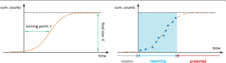
The turning point or inflection point, τ, is defined as the time point when the sign change in the rate of cases accumulation occurs, i.e. changes from increas-ing to decreasincreas-ing or vice versa. Hence, τ is the moment at which the daily (or weekly) incidence trajectory begins to decline, which means the extrinsic growth rate reaches its maximum. The turning point indicates the beginning of an epidemic phase changing from the acceleration to deceleration.

The model parameters K, γ and τ are of epidemiological importance. These parameters can be estimated by fit-ting the growth models to the epidemic data of the ZIKV outbreak. We adopted the standard non-linear least squares (NLS) approach for model fitting and param-eter estimation. Thus, the real cumulative case number at time t, C(t), is assumed to follow a normal distribution

with a mean of the reported cumulative number of cases and an unknown but constant variance [43, 44, 46, 47]. A P-value of < 0.05 is regarded as statistically significant, and the 95% confidence intervals (CI) for all unknown parameters are estimated.

The epidemic data in each state are fitted by all three growth models in Eqns (1–3) (see Fig. 1 for an illustra-tion). We adopted the R2 _{to measure the goodness-of-fit}

of each model. Since the models have different numbers of unknown parameters, the Akaike information crite-rion (AIC) was used to evaluate model performance in terms of the trade-off between the goodness-of-fit and the model complexity. For each state, the model with the lowest AIC value was chosen for further evaluation on its potentials for the real-time estimation.

Reproduction number

The reproduction number, R, is the average number of secondary infectious cases produced by one infectious case during a disease outbreak [40, 45, 60]. When a pop-ulation is totally (i.e. 100%) susceptible, R becomes the basic reproduction number, R0 [39, 61]. When a disease reaches a place (or region) for the first time, the estimated

R can therefore be treated as R0. Following previous stud-ies [38, 40, 60, 62], the reproduction number (R) is given in Eqn (4).

Here, γ is the intrinsic per capita growth rate from the growth model in Eqns (1–3), and κ is the serial inter-val of the ZIKV infection. The serial interinter-val (i.e. gen-eration interval) is the average time interval from onset of one individual to the onset of another individual infected by him/her [44], or the time between succes-sive cases in a chain of transmission [4, 38, 40, 62, 63].

(4)

R₌ 1

M(−γ ) =

1

∫∞0 e−γ κh(κ)dκ .

The function h(∙) represents the probability distribution of the serial interval, κ. Hence, the function M(∙) is the Laplace transform of h(∙), specifically, M(∙) is known to statisticians as the moment generating function (MGF) of a probability distribution.

According to previous work [4], we set h(κ) to be a gamma distribution with a mean of 20.0  days and standard deviation (SD) of 7.4  days, the SDs of the mean and SD of κ are 2.3 and 1.3  days, respectively. Therefore, R can be estimated with the values of γ from models (1–3).

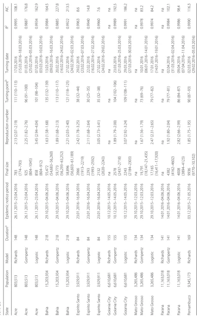
Projection of the epidemic and real‑time estimation

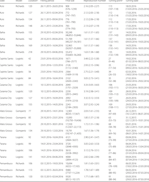
In each state, we chose the model attaining the low-est AIC and simulated it into the future to low-estimate the final size (K) of the outbreak. To evaluate the real-time forecast power, we repeated the fitting procedure start-ing from the full epidemic wave to a sequence of waves with the end week discarded. We denoted the start, the end and the turning pint of the outbreak by 0, T and τ, such that 0 < τ < T. In the fitting part, we used the all data from time 0 to T to fit the models and estimate param-eters. For the real-time estimation, we used the data from time 0 to T1, where 0 < T1 < T, so that the model was fit-ted with an incomplete dataset. With initially T1=T, we decreased T1 gradually from time T backwards until the model fitting diverged. We compared the real-time esti-mated final size (K) and the K estimate based on the com-plete dataset, and stopped the real-time estimation when the yielded confidence interval was too wide (e.g. includ-ing zero) to be useful at the end of epidemic period, i.e. T. We checked the parameter estimates and compared with the results from the full-data modelling to evaluate the analysis sensitivities as the measurement of the real-time estimating potential. The (real-time) estimates with the lowest three T1s were compared to the estimation based on the full dataset.

The knowledge of the turning point (τ) is crucial for real-time projection [44–46], but this information is usu-ally not precisely available. Alternatively, for Zika disease, one may gain knowledge of τ from the mosquito vec-tors’ activities. Since the mosquito abundance in Brazil decreases around May each year [64], we attempted to project the final size (K) with τ fixed at three dates prior to May, namely the first days of February, March and April 2016. Similarly, for the real-time projection, we used the data from time 0 to T1, where 0 < T1 < T, to train the model. The growth model was fitted with the dataset from 0 to T1, and used to project K in real-time. We com-pared the real-time projection of K with the estimates based on full data to measure the forecast power (perfor-mance) of the model.

Results

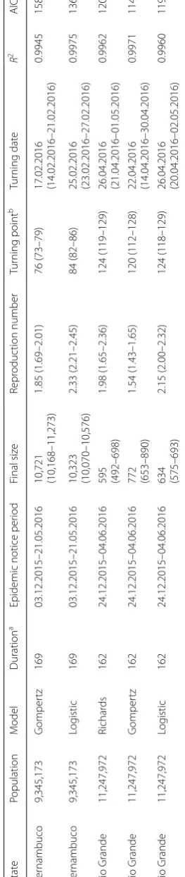
We fitted the three different models in Eqns (1–3) to the time series data of ZIKV incidences number from eight states in Brazil from October 2015 to May 2016. Figure 2 shows that the selected models can provide a good fit to the observations. All selected models achieved a level of

R2 _{larger than 0.995. For each state, we selected the fitting}

results with the lowest value of AIC as the most suitable model (Table 1, Fig. 2). In particular, the Richards model is selected for Acre, Bahia, and Pernambuco; Gompertz model is selected for Mato Grosso and Rio Grande; and the logistic model is selected for Espirito Santo, Goi-ania City and Parana. The reproduction number, R, esti-mates vary from 1.54 to 3.07 for the eight different states (Table 1). We estimate R= 1.54 (95% CI: 1.43–1.65) in Rio

Grande, and R= 3.07 (95% CI: 2.92–3.24) in Goiania City.

The estimated dates of the turning points also vary from January to April of 2016, with 4 out of 8 states in March 2016. For the same state, the final size estimates from dif-ferent models are roughly consistent, with the 95% CIs largely overlapping. The estimated final (epidemic) sizes,

K, are also summarized in Table 1. We estimate the larg-est final outbreak size of 55,472 (95% CI: 54,683–56,260) in Bahia for the outbreak since October 2015, after the one epidemic wave in early 2015 [4, 10].

after the end of disease notification (reporting) period. The epidemic size, K, is the final outbreak size until the end of the epidemic. Moreover, for all states we find that the epidemic sizes estimated 6–35 days after the turning points are indifferent from their final estimations, which means the 95% CIs are largely overlapping (Table 2). This finding indicates that the final outbreak size (K) can be estimated around the epidemic peaking stage by the pro-jections from the simple growth models. By fixing τ to be the first days of February, March and April of 2016, the

K projection converges as more data is including in the model training (Fig. 4). When the assumed turning point becomes closer to the real turning point, the projection of K will gain more accuracy and converges faster even during the early stage of the epidemics (i.e. before the occurrence of the real turning point).

Discussion

We used simple non-linear growth models to study the temporal patterns of ZIKV epidemics in eight Brazil-ian states. We showed that three simple growth models can be adapted to model the ZIKV outbreak, with the best R2 _{reaching 0.995. The estimated dates of the}

turn-ing points varied from January to April of 2016 for the eight states. The difference in the turning points indicates

Table

1

Summar

y table of the model fitting and estimation r

esults

. T

he models r

esults summar

iz

ed her

e ar

e also estimat

ed b

y using the full epidemic dataset dur

ing the whole

epidemic per iod . T he models with the lo w est AICs (for the same stat es) ar e consider ed as main results , which mat ches the results in Fig 2 . T he numbers in par entheses ar e the

95% CIs Stat

e Population M odel Duration a

Epidemic notice per

a T

he

“dur

ation

” is the epidemic r

epor

ting dur

ation (in da

ys) sinc

e the star

ting time (da

te; da

y.mon

th.y

ear) of the r

epor

ted outbr

eak

, which is the diff

er

enc

e of the end and star

t da

tes of the

“epidemic r

epor

ting per

iod

”

b T

he

“tur

ning poin

t”

is the estima

ted time per

iod (in da

ys) fr

om the star

ting time (da

te; da

y.mon

th.y

ear) of the outbr

eak t

o the estima

ted oc

cur

renc

e of the tur

ning poin

t

Abbr

eviations

: AIC, A

kaike inf

or

ma

tion cr

iter

ion; na, not applicable; this oc

curs when the fitting pr

og

ress fails t

o c

on

ver

ge f

or a f

ew model fr

amew

or

ks; CI, c

onfidenc e in ter val Table 1 (c on tinued) Stat e Population M odel Duration a

Epidemic notice per

Table 2 Summary table of the real-time estimation results from the selected models. The model with the lowest AIC (for the same states) is selected for analysis. The models results using the full epidemic dataset during the whole epidemic period match the models

with the lowest AICs in Table 1. The numbers in parentheses are the 95% CIs

State Model Durationa _{Fitting period Final size Reproduction number Turning point}b _{Turning date}

Acre Richards 120 26.11.2015–26.03.2016 908

(576–1239) 2.16 (2.05–2.27) 113(107–118) 18.03.2016(13.03.2016–23.03.2016)

Acre Richards 127 26.11.2015–02.04.2016 772

(747–797) 2.12 (2.05–2.18) 112(110–114) 17.03.2016(15.03.2016–19.03.2016)

Acre Richards 134 26.11.2015–09.04.2016 776

(761–790) 2.12 (2.06–2.18) 112(110–114) 17.03.2016(15.03.2016–19.03.2016)

Acre Richards 148 26.11.2015–23.04.2016 783

(774–793) 2.13 (2.07–2.19) 111(110–113) 17.03.2016(15.03.2016–18.03.2016) Bahia Richards 155 29.10.2015–02.04.2016 50,249

(46,852–53,646) 1.61 (1.57–1.65) 137(131–143) 14.03.2016(09.03.2016–20.03.2016) Bahia Richards 162 29.10.2015–09.04.2016 51,709

(49,237–54,181) 1.61 (1.57–1.66) 137(132–141) 14.03.2016(09.03.2016–19.03.2016) Bahia Richards 169 29.10.2015–16.04.2016 52,963

(50,927–55,000) 1.61 (1.57–1.66) 136(132–141) 14.03.2016(09.03.2016–18.03.2016) Bahia Richards 218 29.10.2015–04.06.2016 55,472

(54,683–56,260) 1.63 (1.58–1.68) 135(132–139) 14.03.2016(09.03.2016–16.03.2016) Espirito Santo Logistic 42 23.01.2016–05.03.2016 1671

(766–2577) 3.48 (2.22–5.30) 27(9–46) 19.02.2016(01.02.2016–08.03.2016) Espirito Santo Logistic 49 23.01.2016–12.03.2016 2126

(1112–3140) 2.93 (2.15–3.96) 35(17–54) 27.02.2016(09.02.2016–16.03.2016) Espirito Santo Logistic 56 23.01.2016–19.03.2016 2364

(1609–3119) 2.75 (2.21–3.40) 39(26–53) 02.03.2016(18.02.2016–15.03.2016) Espirito Santo Logistic 84 23.01.2016–16.04.2016 2132

(2020–2243) 3.05 (2.73–3.41) 35(32–38) 27.02.2016(24.02.2016–29.02.2016) Goiania City Logistic 113 10.12.2015–02.04.2016 2040

(1751–2329) 3.33 (3.05–3.63) 106(102–111) 25.03.2016(21.03.2016–30.03.2016) Goiania City Logistic 120 10.12.2015–09.04.2016 2230

(2015–2445) 3.19 (2.98–3.41) 109(105–112) 28.03.2016(25.03.2016–31.03.2016) Goiania City Logistic 127 10.12.2015–16.04.2016 2092

(1974–2210) 3.32 (3.12–3.53) 107(105–109) 26.03.2016(24.03.2016–28.03.2016) Goiania City Logistic 155 10.12.2015–14.05.2016 2243

(2184–2303) 3.07 (2.92–3.24) 109(108–111) 29.03.2016(27.03.2016–30.03.2016) Mato Grosso Gompertz 77 29.10.2015–14.01.2016 12,901

(8235–17,567) 2.03 (1.61–2.55) 58(47–69) 26.12.2015(16.12.2015–06.01.2016) Mato Grosso Gompertz 85 29.10.2015–23.01.2016 15,093

(10,750–19,436) 1.85 (1.57–2.18) 63(53–73) 31.12.2015(22.12.2015–10.01.2016) Mato Grosso Gompertz 92 29.10.2015–30.01.2016 17,550

(12,927–22,172) 1.72 (1.51–1.96) 68(58–78) 05.01.2016(26.12.2015–15.01.2016) Mato Grosso Gompertz 134 29.10.2015–12.03.2016 19,791

(18,147–21,435) 1.67 (1.56–1.79) 73(69–76) 10.01.2016(06.01.2016–14.01.2016) Parana Logistic 92 14.01.2016–16.04.2016 4121

(2604–5637) 2.90 (2.41–3.47) 86(73–99) 09.04.2016(27.03.2016–22.04.2016) Parana Logistic 99 14.01.2016–23.04.2016 3720

(3048–4393) 3.05 (2.63–3.53) 82(75–89) 06.04.2016(30.03.2016–13.04.2016) Parana Logistic 106 14.01.2016–30.04.2016 3610

(3228–3992) 3.12 (2.76–3.51) 81(77–86) 05.04.2016(31.03.2016–09.04.2016) Parana Logistic 141 14.01.2016–04.06.2016 4008

(3894–4123) 2.82 (2.66–2.99) 86(84–87) 09.04.2016(07.04.2016–11.04.2016) Pernambuco Richards 106 03.12.2015–19.03.2016 10,694

(4222–17,165) 1.81 (1.63–2.01) 94(78–109) 06.03.2016(19.02.2016–22.03.2016) Pernambuco Richards 113 03.12.2015–26.03.2016 9480

(7737–11,224) 1.78 (1.67–1.89) 91(88–95) 04.03.2016(29.02.2016–07.03.2016) Pernambuco Richards 120 03.12.2015–02.04.2016 9320

the timely efficiency of the local ZIKV notification, we checked if the turning point appeared in the latter half of the whole reporting period. This can be simply quan-tified by calculating the ratio of the “turning point” over “duration” in Table 1, and compared with 0.5. Most of the

states had a turning point in the latter half of the outbreak reporting period except for the state of Espirito Santo. Espirito Santo had a turning point (τ) in the former half of the epidemic period (T) significantly, i.e. τ < T/2, which is different from other states, thus an outlier.

a _{The “duration” is the fitting duration (in days) since the starting time (date; day.month.year) for fitting, which is the difference of the end and start dates of the “fitting} period”

b _{The “turning point” is the estimated time period (in days) from the starting time (date; day.month.year) of the outbreak to the estimated occurrence of the turning} point

Table 2 (continued)

State Model Durationa _{Fitting period Final size Reproduction number Turning point}b _{Turning date}

Pernambuco Richards 169 03.12.2015–21.05.2016 9936

(9770–10,102) 1.85 (1.75–1.95) 90(87–93) 02.03.2016(29.02.2016–05.03.2016) Rio Grande Gompertz 148 24.12.2015–21.05.2016 771

(563–979) 1.54 (1.39–1.71) 120(107–134) 22.04.2016(09.04.2016–06.05.2016) Rio Grande Gompertz 155 24.12.2015–28.05.2016 765

(613–917) 1.54 (1.42–1.68) 120(110–130) 22.04.2016(12.04.2016–02.05.2016) Rio Grande Gompertz 162 24.12.2015–04.06.2016 772

(653–890) 1.54 (1.43–1.65) 120(112–128) 22.04.2016(14.04.2016–30.04.2016)

The disease infectivity is measured by the reproduction number, R, during an outbreak (Table 1). The estimated

R-values are significantly less than 2 (with 95% CIs lower than 2) in the four states of Bahia, Mato Grosso, Pernam-buco and the Rio Grande. The Rs are significantly larger than 2 in the four states of Acre, Espirito Santo, Goiania City and Parana. In states of Bahia, Mato Grosso and Per-nambuco, there were ZIKV cases confirmed since early 2015 [4]. Thus, the lower R-values are likely to be due to the depletion of susceptible population during the ear-lier outbreaks. In the state of Rio Grande, one possible explanation for the lowest R= 1.54 (95% CI: 1.43–1.65) is the relatively lower air temperature than most of the other places in Brazil. The average temperature starts to drop below 20 °C from March every year, during which the mosquito vector abundance is almost zero [65]. For the four states of Acre, Espirito Santo, Goiania City and

Parana, ZIKV was not reported before October 2015 [4], and thus the R-values can also be treated as the esti-mates of the basic reproduction number, R0. Hence, we speculate that the R0 of ZIKV ranges from 2.07 to 3.41 by directly finding the range of the 95% CIs of R-values in states of Acre, Espirito Santo, Goiania City and Parana. The average value of R0 was 2.77. This average value and range of R0 is consistent with previous ZIKV studies for Brazil [4, 12, 14].

estimation. Moreover, for all states, the epidemic sizes estimated 6–35  days after the turning points are virtu-ally indifferent from their final estimations (i.e. estimates of K by using the full dataset). These findings reveal the real-time estimating potentials for the simple growth models proposed in this study. The final epidemic size (K) can be predicted at or after the peaking time of the epi-demic. The early prediction of the final outbreak size (K) was found to depend on the timing of the turning point (τ), as shown in Fig. 3. Although projecting the tempo-ral trends of an outbreak from the early-stage incomplete dataset could be sometimes misleading, we note that the predictions are reasonably accurate when the fitting dataset covers the turning point, which is in-line with the findings in [46, 66]. With data coming in from an ongoing outbreak, the performance of models used in this work will be continuously improved, thus real-time estimates of key epidemiological parameters may be available before the epidemic fully ends.

Since the prediction should be before the occurrence of an event, we note that the turning points forecast is difficult to be achieved with the simple models, which was also reported by previous Zika and dengue model-ling literature [44, 45]. Nevertheless, we highlight the importance of a successful turning point forecast in the prediction of other epidemiological parameters. Our findings suggest that the projection on the epidemic final size (K) converges after using the data with time duration slightly over the turning point. In other words, once the knowledge of the turning point is equipped, the real-time estimation can be largely improved and con-verges quickly. To estimate the turning point (τ) we may not only rely on surveillance case data but also take into account of practical knowledge and factors that affect the disease transmission. For instance, the Zika fever in this work is a disease whose transmission depends largely on the activity of mosquitoes, which has strong seasonality. Local mosquito abundance drops to a sufficiently low level from May each year [64], which could largely reduce the ZIKV spread. Hence, τ is probably before May 2016. By fixing τ on the first day of February, March and April 2016, the K projection converges as more data is included in the training of the model (Fig. 4). When the assumed turning point approaches the real turning point, the pro-jection of K will approach the estimate based on full data, and converge faster even during the early stage of the epi-demics, i.e. before the arrival of the real turning point.

Besides the three models adopted in this study, there are other well-known non-linear growth models that have not been adopted. These unselected models include the four-parameter logistic, five-parameter logistic, Weibull and Sigmoid Emax models. One of the facts of the S-shape epidemic curve is that the growth starts from

level zero. The Weibull and Sigmoid Emax models are more likely to yield inferior fitting performance with zero lower asymptote (or bound). Besides, the Sigmoid Emax model does not contain an intrinsic growth term. Thus, these two models are less popular in studying epidemic curves than the three models in Eqns (1–3). For the four-parameter logistic model, it is equivalent to the three-parameter version in Eqn (1) when the lower asymptote becomes zero. Although the five-parameter logistic model adds asymmetry factor (to control the asymmetry) based on the four-parameter version [67], it still contains the non-zero lower asymptote problem [68]. In addition, the five-parameter logistic model also could be over-sensitive for the early-stage prediction [46]. These short-comings make it less practical than the Richards model in studying the epidemic curve. Therefore, we only adopt the three growth models in Eqns (1–3).

This work has some limitations. The analyses are highly reliant on the quality of the epidemic data, reporting delay and the change of reporting criteria. Since the local ZIKV surveillance are more reliable after the end of 2015 [26], we modeled the single-wave outbreaks on or after October 2015 and avoid including the dataset during early 2015. Due to the interference with the other Fla-vivirus (e.g. dengue virus, yellow fever virus, West Nile virus, etc.) [69], the serological diagnosis of ZIKV infec-tion is less effective than the RT-PCR diagnosis. How-ever, the time window for positive RT-PCR viremia is relatively short, roughly three to seven days, thus a sus-pected ZIKV should not be regarded as a negative case, which requires IgM tests for further confirmation [69]. Therefore, to avoid excluding the part of positive ZIKV cases in the suspected group, we considered the summa-tion of suspected and confirmed cases as the incidence count for analysis. If the reporting delays, dates of onset, or the reporting rate are known, more realistic and com-prehensive analysis can be performed that includes more accurate epidemic data and information. In this idealistic situation, although our simple non-linear models would be less attractive, they still could be used as the baseline framework for more advanced analysis, and to estimate the turning points.

Conclusions

real-time projection of the final size is likely to be more accurate, even during the early stage of epidemics. Our modelling framework may be extended to study other infectious diseases epidemics, and easily implemented for a practical purpose.

Additional file

Additional file 1: Text S1. The difference between the three growth models.

Abbreviations

ZIKV: Zika virus; CI: confidence interval; EW: epidemiological week; MGF: moment generating function; SD: standard deviation; AIC: Akaike information criterion; NLS: non-linear least squares; GBS: Guillain-Barré syndrome.

Acknowledgements

Not applicable.

Authors’ contributions

SZ conceived and carried out the study, and drafted the first manuscript. SZ and DH discussed the results. SZ, SSM, HF, DH and JQ revised the manuscript. All authors read and approved the final manuscript.

Funding

The work described in this paper was partly supported by a grant from The Hong Kong Polytechnic University (Project no.: 1-ZE8J). The funding agencies had no role in the design and conduct of the study; collection, management, analysis, or interpretation of the data; preparation, review, or approval of the manuscript; or decision to submit the manuscript for publication.

Availability of data and materials

All data used for analysis are freely available in the supplementary materials of Ferguson et al. [4].

Ethics approval and consent to participate

Since no personal data were collected, ethical approval or individual consent was not required.

Consent for publication

Not applicable.

Competing interests

The authors declare that they have no competing interests.

Author details

1 _{School of Nursing, Hong Kong Polytechnic University, Hong Kong, China.} 2 _{Department of Applied Mathematics, Hong Kong Polytechnic University,}

Hong Kong, China. 3 _{Department of Crop Science and Technology, College}

of Agriculture, South China Agricultural University, Guangzhou, China.

Received: 5 March 2019 Accepted: 6 July 2019

References

1. Dick G, Kitchen S, Haddow A. Zika virus (I). Isolations and serological specificity. Trans R Soc Trop Med Hyg. 1952;46:509–20.

2. Moore D, Causey O, Carey D, Reddy S, Cooke A, Akinkugbe F, et al. Arthropod-borne viral infections of man in Nigeria, 1964–1970. Ann Trop Med Parasitol. 1975;69:49–64.

3. Wikan N, Smith DR. Zika virus: history of a newly emerging arbovirus. Lancet Infect Dis. 2016;16:e119–26.

4. Ferguson NM, Cucunubá ZM, Dorigatti I, Nedjati-Gilani GL, Donnelly CA, Basáñez M-G, et al. Countering the Zika epidemic in Latin America. Sci-ence. 2016;353:353–4.

5. Mlakar J, Korva M, Tul N, Popović M, Poljšak-Prijatelj M, Mraz J, et al. Zika virus associated with microcephaly. N Engl J Med. 2016;374:951–8. 6. Monaghan AJ, Morin CW, Steinhoff DF, Wilhelmi O, Hayden M, Quattrochi

DA, et al. On the seasonal occurrence and abundance of the Zika virus vector mosquito Aedes aegypti in the contiguous United States. PLoS Curr. 2016. https ://doi.org/10.1371/curre nts.outbr eaks.50dfc 7f467 98675 fc63e 7d7da 563da 76.

7. Petersen LR, Jamieson DJ, Powers AM, Honein MA. Zika virus. N Engl J Med. 2016;374:1552–63.

8. Duffy MR, Chen T-H, Hancock WT, Powers AM, Kool JL, Lanciotti RS, et al. Zika virus outbreak on Yap Island, federated states of Micronesia. N Engl J Med. 2009;360:2536–43.

9. Aubry M, Teissier A, Huart M, Merceron S, Vanhomwegen J, Roche C, et al. Zika virus seroprevalence, French Polynesia, 2014–2015. Emerg Infect Dis. 2017;23:669.

10. He D, Gao D, Lou Y, Zhao S, Ruan S. A comparison study of Zika virus outbreaks in French Polynesia, Colombia and the State of Bahia in Brazil. Sci Rep. 2017;7:273.

11. Campos GS, Bandeira AC, Sardi SI. Zika virus outbreak, Bahia, Brazil. Emerg Infect Dis. 2015;21:1885.

12. Gao D, Lou Y, He D, Porco TC, Kuang Y, Chowell G, et al. Prevention and control of Zika as a mosquito-borne and sexually transmitted disease: a mathematical modeling analysis. Sci Rep. 2016;6:28070.

13. Ikejezie J, Shapiro CN, Kim J, Chiu M, Almiron M, Ugarte C, et al. Zika virus transmission—region of the Americas, May 15, 2015–December 15, 2016. MMWR Morb Mortal Wkly Rep. 2017;66:329.

14. Zhang Q, Sun K, Chinazzi M, Pastore y Piontti A, Dean NE, Rojas DP, et al. Spread of Zika virus in the Americas. Proc Natl Acad Sci USA. 2017;114:E4334–43.

15. Towers S, Brauer F, Castillo-Chavez C, Falconar AK, Mubayi A, Romero-Vivas CM. Estimate of the reproduction number of the 2015 Zika virus outbreak in Barranquilla, Colombia, and estimation of the relative role of sexual transmission. Epidemics. 2016;17:50–5.

16. Atkinson B, Hearn P, Afrough B, Lumley S, Carter D, Aarons EJ, et al. Detec-tion of Zika virus in semen. Emerg Infect Dis. 2016;22:940.

17. WHO. Zika virus. Geneva: World Health Organization; 2019. https ://www. who.int/news-room/fact-sheet s/detai l/zika-virus . Accessed 1 Apr 2019. 18. Cao-Lormeau V-M, Blake A, Mons S, Lastère S, Roche C, Vanhomwegen J,

et al. Guillain-Barré syndrome outbreak associated with Zika virus infec-tion in French Polynesia: a case–control study. Lancet. 2016;387:1531–9. 19. de Paula Freitas B, de Oliveira Dias JR, Prazeres J, Sacramento GA, Ko AI,

Maia M, et al. Ocular findings in infants with microcephaly associated with presumed Zika virus congenital infection in Salvador, Brazil. JAMA Ophthalmol. 2016;134:529–35.

20. Plourde AR, Bloch EM. A literature review of Zika virus. Emerg Infect Dis. 2016;22:1185.

21. dos Santos T, Rodriguez A, Almiron M, Sanhueza A, Ramon P, de Oliveira WK, et al. Zika virus and the Guillain-Barré syndrome—case series from seven countries. N Engl J Med. 2016;375:1598–601.

22. Cauchemez S, Besnard M, Bompard P, Dub T, Guillemette-Artur P, Eyrolle-Guignot D, et al. Association between Zika virus and micro-cephaly in French Polynesia, 2013–15: a retrospective study. Lancet. 2016;387:2125–32.

23. Brasil P, Pereira JP Jr, Moreira ME, Ribeiro Nogueira RM, Damasceno L, Wakimoto M, et al. Zika virus infection in pregnant women in Rio de Janeiro. N Engl J Med. 2016;375:2321–34.

24. de Oliveira WK, Carmo EH, Henriques CM, Coelho G, Vazquez E, Cortez-Escalante J, et al. Zika virus infection and associated neurologic disorders in Brazil. N Engl J Med. 2017;376:1591–3.

25. Pan American Health Organization (PAHO), World Health Organization (WHO). Zika—Epidemiological report Brazil; 2017. https ://www.paho.org/ hq/dmdoc ument s/2017/2017-phe-zika-situa tion-repor t-bra.pdf. 2019. 26. The Reuters, The News press entitled “Exclusive: Brazil says Zika virus

outbreak worse than believed”, 2016. http://www.reute rs.com/artic le/ us-healt h-zika-brazi l-exclu sive-idUSK CN0VA 331. 2019.

28. de Oliveira WK. Increase in reported prevalence of microcephaly in infants born to women living in areas with confirmed Zika virus transmis-sion during the first trimester of pregnancy—Brazil, 2015. MMWR Morb Mortal Wkly Rep. 2016;65:242–7.

29. van der Linden V. Description of 13 infants born during October 2015– January 2016 with congenital Zika virus infection without microcephaly at birth—Brazil. MMWR Morb Mortal Wkly Rep. 2016;65:1343–8. 30. de Oliveira WK, de França GVA, Carmo EH, Duncan BB, de Souza

Kuchen-becker R, Schmidt MI. Infection-related microcephaly after the 2015 and 2016 Zika virus outbreaks in Brazil: a surveillance-based analysis. Lancet. 2017;390:861–70.

31. Hollingsworth TD, Pulliam JR, Funk S, Truscott JE, Isham V, Lloyd AL. Seven challenges for modelling indirect transmission: vector-borne diseases, macroparasites and neglected tropical diseases. Epidemics. 2015;10:16–20.

32. Earn DJ, Brauer F, van den Driessche P, Wu J. Mathematical epidemiology. Berlin: Springer; 2008.

33. Brauer F, Castillo-Chavez C. Mathematical models in population biology and epidemiology, vol. 40. Berlin: Springer; 2012.

34. Keeling MJ, Rohani P. Modeling infectious diseases in humans and ani-mals. Princeton: Princeton University Press; 2011.

35. Riley S, Fraser C, Donnelly CA, Ghani AC, Abu-Raddad LJ, Hedley AJ, et al. Transmission dynamics of the etiological agent of SARS in Hong Kong: impact of public health interventions. Science. 2003;300:1961–6. 36. Zhao S, Stone L, Gao D, He D. Modelling the large-scale yellow fever

outbreak in Luanda, Angola, and the impact of vaccination. PLoS Negl Trop Dis. 2018;12:e0006158.

37. Lin Q, Chiu AP, Zhao S, He D. Modeling the spread of Middle East respira-tory syndrome coronavirus in Saudi Arabia. Stat Methods Med Res. 2018;27:1968–78.

38. Fraser C. Estimating individual and household reproduction numbers in an emerging epidemic. PLoS ONE. 2007;2:e758.

39. Van den Driessche P, Watmough J. Reproduction numbers and sub-threshold endemic equilibria for compartmental models of disease transmission. Math Biosci. 2002;180:29–48.

40. Wallinga J, Lipsitch M. How generation intervals shape the relation-ship between growth rates and reproductive numbers. Proc Biol Sci. 2006;274:599–604.

41. Arino J, Brauer F, Van Den Driessche P, Watmough J, Wu J. A final size rela-tion for epidemic models. Math Biosci Eng. 2007;4:159.

42. Ma J, Earn DJ. Generality of the final size formula for an epidemic of a newly invading infectious disease. Bull Math Biol. 2006;68:679–702. 43. Hsieh Y-H. Richards model: a simple procedure for real-time prediction of

outbreak severity. In: Ma Z, Zhou Y, Wu J, editors. Modeling and dynamics of infectious diseases. Singapore: World Scientific; 2009. p. 216–36. 44. Hsieh Y-H. Temporal patterns and geographic heterogeneity of Zika

virus (ZIKV) outbreaks in French Polynesia and Central America. PeerJ. 2017;5:e3015.

45. Hsieh Y-H, Ma S. Intervention measures, turning point, and reproduction number for dengue, Singapore, 2005. Am J Trop Med Hyg. 2009;80:66–71. 46. Sebrango-Rodríguez CR, Martínez-Bello DA, Sánchez-Valdés L,

Thila-karathne PJ, Del Fava E, Van Der Stuyft P, et al. Real-time parameter estimation of Zika outbreaks using model averaging. Epidemiol Infect. 2017;145:2313–23.

47. Zhou G, Yan G. Severe acute respiratory syndrome epidemic in Asia. Emerg Infect Dis. 2003;9:1608–10.

48. Funk S, Camacho A, Kucharski AJ, Eggo RM, Edmunds WJ. Real-time forecasting of infectious disease dynamics with a stochastic semi-mecha-nistic model. Epidemics. 2018;22:56–61.

49. Tizzoni M, Bajardi P, Poletto C, Ramasco JJ, Balcan D, Gonçalves B, et al. Real-time numerical forecast of global epidemic spreading: case study of 2009 A/H1N1pdm. BMC Med. 2012;10:165.

50. Yang W, Cowling BJ, Lau EH, Shaman J. Forecasting influenza epidemics in Hong Kong. PLoS Comput Biol. 2015;11:e1004383.

51. Hsieh Y-H, Cheng Y-S. Real-time forecast of multiphase outbreak. Emerg Infect Dis. 2006;12:122.

52. Nishiura H, Chowell G, Safan M, Castillo-Chavez C. Pros and cons of estimating the reproduction number from early epidemic growth rate of influenza A (H1N1) 2009. Theor Biol Med Model. 2010;7:1.

53. Liao JJ, Liu R. Re-parameterization of five-parameter logistic function. J Chemom. 2009;23:248–53.

54. WHO. The interim case definition of Zika virus disease. Geneva: World Health Organization. 2019; https ://www.who.int/csr/disea se/zika/case-defin ition /en/. 2019.

55. Brazilian Institute of Geography and Statistics. The Resident population figures sent to the Brazilian Court of Audit from 2001 to 2015; 2019. ftp://ftp.ibge.gov.br/Estim ativa s_de_Popul acao/Estim ativa s_2015/serie _2001_2015_TCU.pdf. Accessed 1 Apr 2019.

56. Verhulst P. La loi d’accroissement de la population. Nouv Mem Acad Roy Soc Belle-lettr Bruxelles. 1845;18:1–38.

57. Gompertz B. XXIV. On the nature of the function expressive of the law of human mortality, and on a new mode of determining the value of life contingencies. In a letter to Francis Baily, Esq. FRS &c. Philos Trans R Soc Lond. 1825;115:513–83.

58. Richards F. A flexible growth function for empirical use. J Exp Bot. 1959;10:290–301.

59. Tsoularis A, Wallace J. Analysis of logistic growth models. Math Biosci. 2002;179:21–55.

60. Ma J, Dushoff J, Bolker BM, Earn DJ. Estimating initial epidemic growth rates. Bull Math Biol. 2014;76:245–60.

61. Fraser C, Donnelly CA, Cauchemez S, Hanage WP, Van Kerkhove MD, Hol-lingsworth TD, et al. Pandemic potential of a strain of influenza A (H1N1): early findings. Science. 2009;324:1557–61.

62. Wallinga J, Teunis P. Different epidemic curves for severe acute respiratory syndrome reveal similar impacts of control measures. Am J Epidemiol. 2004;160:509–16.

63. Fine PE. The interval between successive cases of an infectious disease. Am J Epidemiol. 2003;158:1039–47.

64. Paes de Andrade P, Aragão FJL, Colli W, Dellagostin OA, Finardi-Filho F, Hirata MH, et al. Use of transgenic Aedes aegypti in Brazil: risk perception and assessment. Bull World Health Organ. 2016;94:766–71.

65. Beck-Johnson LM, Nelson WA, Paaijmans KP, Read AF, Thomas MB, Bjørnstad ON. The effect of temperature on Anopheles mosquito popula-tion dynamics and the potential for malaria transmission. PLoS ONE. 2013;8:e79276.

66. Hsieh Y-H, Lee J-Y, Chang H-L. SARS epidemiology modeling. Emerg Infect Dis. 2004;10:1165.

67. Gottschalk PG, Dunn JR. The five-parameter logistic: a characteriza-tion and comparison with the four-parameter logistic. Anal Biochem. 2005;343:54–65.

68. Rozema E. Epidemic models for SARS and measles. College Math J. 2007;38:246–59.

69. WHO. Laboratory testing for Zika virus infection: interim guidance. Geneva: World Health Organization; 2019. https ://www.who.int/csr/resou rces/publi catio ns/zika/labor atory -testi ng/en/. Accessed 1 Apr 2019.

Publisher’s Note