Modeling and synthesis of the HD photo compression algorithm

(1)

Rochester Institute of Technology

RIT Scholar Works

Theses

Thesis/Dissertation Collections

8-1-2008

Modeling and synthesis of the HD photo

compression algorithm

Seth Groder

Follow this and additional works at:

http://scholarworks.rit.edu/theses

This Thesis is brought to you for free and open access by the Thesis/Dissertation Collections at RIT Scholar Works. It has been accepted for inclusion

in Theses by an authorized administrator of RIT Scholar Works. For more information, please contact

[email protected]

.

Recommended Citation

(2)

Modeling and Synthesis of the HD Photo Compression Algorithm

by

Seth Groder

A Thesis Submitted

in

Partial Fulfillment of the

Requirements for the Degree of

MASTERS OF SCIENCE

in

Computer Engineering

Approved by:

Principal Advisor

________________________________________________

Dr. Kenneth Hsu, RIT Department of Computer Engineering

Committee Member

_____________________________________________

Dr. Muhammad Shaaban, RIT Department of Computer Engineering

Committee Member

_____________________________________________

Mr. Francis Tse, Xerox Corporation

Department of Computer Engineering

College of Engineering

Rochester Institute of Technology

Rochester, New York

(3)

RELEASE PERMISSION FORM

Rochester Institute of Technology

Modeling and Synthesis of the HD Photo Compression Algorithm

I, Seth

Groder, hereby grant permission to the Wallace Library and the Department of Computer

Engineering at the Rochester Institute of Technology to reproduce my thesis in whole or in part.

Any reproduction in these accounts will not be for commercial use or profit.

____________________________________________

Seth Groder

(4)

i

Abstract

The primary goal of this thesis is to implement the HD Photo encoding algorithm using Verilog

HDL in hardware. The HD Photo algorithm is relatively new and offers several advantages over

other digital still continuous tone image compression algorithms and is currently under review by

the JPEG committee to become the next JPEG standard, JPEG XR.

HD Photo was chosen to become the next JPEG standard because it has a computationally light

domain change transform, achieves high compression ratios, and offers several other

improvements like its ability to supports a wide variety of pixel formats. HD Photo’s

compression algorithm has similar image path to that of the baseline JPEG but differs in a few

key areas. Instead of a discrete cosine transform HD Photo leverages a lapped biorthogonal

transform. HD Photo also has adaptive coefficient prediction and scanning stages to help furnish

high compression ratios at lower implementation costs.

In this thesis, the HD Photo compression algorithm is implemented in Verilog HDL, and three

key stages are further synthesized with Altera’s Quartus II design suite with a target device of a

Stratix III FPGA. Several images are used for testing for quality and speed comparisons between

HD Photo and the current JPEG standard using the HD Photo plug-in for Adobe’s Photoshop

CS3. The compression ratio when compared to the current baseline JPEG standard is about 2x so

the same quality image can be stored in half the space. Performance metrics are derived from the

Quartus II synthesis results. These are approximately 108,866 / 270,400 ALUTs (40%), a 10 ns

(5)

ii

Acknowledgements

The author would like to acknowledge all of the direction, guidance, and assistance he has

received from his thesis committee, Dr Ken Hsu, Dr. Muhammad Shaaban, and Mr. Francis Tse,

whom without which this thesis would not have come together. The author would also like to

express his gratitude and appreciation for the support he has received from his friends and family

(6)

iii

Bitstream Structure ... 12

1.3.5

Supported Features... 13

2

Design... 14

2.1

Constraints ... 14

2.2

Image Setup ... 15

2.3

Color Transform... 15

2.4

Lapped Biorthogonal Transform... 16

2.4.1

Photo Core Transform... 19

2.4.2

Photo Overlap Transform ... 23

(7)

iv

2.6

Adaptive Coefficient Prediction ... 27

2.7

Adaptive Coefficient Scanning ... 29

2.8

Adaptive Entropy Encoding ... 31

2.9

Adaptive Coefficient Normalization ... 33

3

Implementation ... 34

3.1

Lapped Biorthogonal Transform... 34

3.1.1

General Transform Information... 34

3.1.2

Photo Core Transform... 35

3.1.3

Photo Overlap Transform ... 38

3.1.4

16x16 Lapped Biorthogonal Transform... 40

3.2

Quantization ... 43

3.2.1

Quant Map ... 43

3.2.2

4x4 Quantizer... 44

3.3

Adaptive Coefficient Prediction ... 45

3.4

Adaptive Coefficient Scanning ... 47

3.5

Adaptive Entropy Encoding ... 48

3.5.1

DC Encoder... 48

3.5.2

LP Encoder... 49

3.5.3

HP Encoder ... 50

4

Verification ... 52

4.1

Verilog Testbench... 52

4.2

Software Models... 54

5

Results ... 55

5.1

Layout Analysis ... 55

5.2

Performance Analysis ... 55

5.3

Power Analysis... 57

5.4

Compression Analysis ... 58

6

Conclusion and Future Work... 60

6.1

Project Benefits ... 60

(8)

v

6.3

Possible Enhancements ... 62

References ... 64

Appendix A. Images... 66

thumbnail.bmp... 66

tree.tiff ... 66

lenna.tiff... 67

shea.bmp... 68

Appendix B. VHDL Code... 69

lbt_16x16.v ... 69

predict_16x16.v ... 85

scanner_16x16.v... 95

Appendix C. Perl Script ... 100

bmp_to_hex.pl ... 100

Appendix D. Quartus II Synthesis Reports ... 101

LBT Fitting:... 101

LBT Timing: ... 101

LBT Power: ... 101

Prediction Fitting:... 102

Prediction Timing: ... 102

Prediction Power: ... 103

Scanning Fitting:... 103

Scanning Timing: ... 103

(9)

vi

List of Figures

Figure 1.1. JPEG and HD Photo Compression Steps [17]... 7

Figure 1.2. Spatial Layout of Macroblock Aligned Image [13,18] ... 11

Figure 1.3. Process of Developing Frequency Hierarchy ... 12

Figure 1.4. HD Photo Bitstream Structure [13,15] ... 13

Figure 2.1. PCT and POT Operation Boundaries [14]... 17

Figure 2.2. Various LBT Implementation Techniques ... 18

Figure 2.3. Pseudo-code for 2x2 Hadamard Transform [13]... 20

Figure 2.4. Pseudo-code for 2x2 Odd Transform [13]... 21

Figure 2.5. Pseudo-code for 2x2 Odd-Odd Transform [13] ... 22

Figure 2.6. Pseudo-code for 4x4 PCT [13] ... 23

Figure 2.7. Pseudo-code for 2-Point Rotation Transform [13]... 24

Figure 2.8. Pseudo-code for 2-Point Scaling Transform [13]... 24

Figure 2.9. Pseudo-code for 4-Point POT [13] ... 25

Figure 2.10. Pseudo-code for 4x4 POT [13]... 26

Figure 2.11. DC Prediction Layout [15] ... 28

Figure 2.12. LP Coefficient Prediction [15] ... 28

Figure 2.13. HP Left Prediction Scheme [14,15]... 29

Figure 2.14. Initial Scan Patterns (a) LP and HP Horizontal (b) HP Vertical [15] ... 30

Figure 2.15. Example of Adaptive Coefficient Scanning [15] ... 31

Figure 2.16. Example 3½D - 2½D Coded Stream [15] ... 31

Figure 2.17. VLC Coding Tables used by HD Photo [13,14,15]... 32

Figure 2.18. Coefficient Normalization Process [13,15] ... 33

Figure 3.1. Structural Overview of 2x2 Hadamard Transform... 35

Figure 3.2. Structural Overview of 2x2 Odd Transform ... 36

Figure 3.3. Structural Overview of 2x2 Odd-Odd Transform ... 36

Figure 3.4. Structural Overview of 4x4 PCT... 37

Figure 3.5. Structural Overview of 2-Point Rotation... 38

Figure 3.6. Structural Overview of 2-Point Scaling ... 38

Figure 3.7. Structural Overview of 4-Point POT... 39

Figure 3.8. Structural Overview of 4x4 POT... 40

Figure 3.9.Structural Overview of LBT... 42

Figure 3.10. Structural Overview of Quant Map ... 44

Figure 3.11. Structural Overview of 4x4 Quantizer ... 45

Figure 3.12. Structural Overview of Adaptive Coefficient Prediction ... 46

Figure 3.13. Structural Overview of Adaptive Coefficient Scanner... 47

Figure 3.14. Structural Overview of DC Encoder ... 49

Figure 3.15. Structural Overview of Run-Length Encoder with Flexbit Support ... 50

Figure 3.16. Structural Overview of HP Encoder... 51

Figure 4.1. Testbench Simulation Environment ... 53

Figure 5.1. Chart of Compression Time vs. Amount of Pixels in the Image... 57

(10)

vii

List of Tables

Table 1.1. Complete List of Supported Pixel Formats [13]... 9

Table 1.2. Illustration of Combination of Rotate and Flips [15] ... 13

Table 5.1. Layout Results of Design Modules... 55

Table 5.2. Performance Analysis of Design Modules ... 56

Table 5.3. Sample Image Completion Times... 57

Table 5.4. Power Analysis of Design Modules... 58

(11)

viii

Glossary

ASIC:

Application Specific Integrated Circuit – An integrated circuit that was

developed for a specific purpose that could not be achieved within an

off-the-shelf part.

Bit stream:

Term used to describe a series of bits that are produced as a result of the

encoding process.

BGR:

Blue Green Red – A pixel format describing the order of three color planes.

Block:

A 4x4 matrix of coefficient data co-located across all color channels

BMP:

File extension used to denote a bitmap file format.

CBP:

Coded Block Pattern – Encoded series of bits that detail on which portion of the

image contains meaningful data.

Codec:

A combination of both an encoder and decoder

DCT:

Discrete Cosine Transform – 8x8 block transform utilized by the baseline JPEG

standard

DWT:

Discrete Wavelet Transform – Wavelet transform utilized by the JPEG 2000

standard

FPGA:

Field Programmable Gate Array – Chip which usually contains numerous LUT’s

and memory.

HDL:

Hardware Description Language – Description of a computer language that is

commonly used to design and test analog, digital, and mixed-signal circuits.

HDP:

HD Photo – Image codec and file format standard developed by Microsoft. Also

may be used as the file extension.

HDR:

High Dynamic Range – Term used to describe pixel formats that can represent a

significantly amount of colors by using more bits per pixel.

HEX:

File extension used for files containing a series of hexadecimal number values.

ISO:

International Organization for Standardization – Non-governmental organization

that sets international standards for a wide range of applications.

(12)

ix

produced by the group.

LBT:

Lapped Biorthogonal Transform – Main 2 stage reversible transform leveraged

in the HD Photo compression algorithm to change domains.

LUT:

Lookup Table – A data structure that replaces a runtime operation with a simpler

indexing operation.

Macroblock:

A 4x4 matrix of blocks, which subsequently makes a 16x16 matrix of coefficient

data co-located across all color channels

MFP:

Multifunction Printer – Device usually capable of more than just printing,

including such features as scanning, copying, and faxing.

PCT:

Photo Core Transform – 4x4 block transform utilized within the two stages of

the LBT

POT:

Photo Overlap Transform – 4x4 block transform that may occur within the LBT

across block boundaries to reduce blocking artifacts within the compressed

image.

QP:

Quantization Parameter – Describes a single or set of values used in the

quantization stage of the algorithm

RGB:

Red Green Blue – A pixel format describing the order of three color planes.

ROI:

Region of Interest – Refers to the ability to access specific pixels from within a

compressed bitstream.

VLC:

Variable Length Code – Term used to describe an encoding pattern that replaces

fixed length elements with elements that vary in bit depth with the intention of

reducing the total bits.

YUV:

Color space using three channels, one

luma

, y, and two

chroma

, u & v.

YUV420:

YUV colorspace where a sample of the

luma

channel is a 4x4 matrix of pixel

data and the

chroma

channels are sub sampled with only 2x2 matrices of pixel

data.

YUV422:

YUV colorspace where a sample of the

luma

channel is a 4x4 matrix of pixel

data and the

chroma

channels are sub sampled with only 4x2 matrices of pixel

data.

(13)

1

Introduction

As technology improves and the demand for image quality increases the topic of efficient image

compression is as relevant as ever. Many image compression algorithms are ill equipped to

handle new high dynamic range (HDR) and wide gamut formats because their algorithms were

developed with a generic three color channel eight bits of pixel data per channel model. New

color formats may use 16 or even 32 bits per color channel and in some cases there are more than

three color channels. This new image compression paradigm provides motivation to create a

versatile compression algorithm that is capable of accommodating the majority of the color

format spectrum while still remaining computationally efficient and portable.

The JPEG committee has been responsible for overseeing and developing new digital image

compression algorithms for almost two decades. The committee was formed in 1986 and had its

original lossy JPEG standard that is still widely used today, ISO 10918-1

,

was under

development in 1990 accepted in 1994 [4,8,18]. Since then there have been modified versions

that standard that have allowed lossless encoding and 12-bits of data per color channel. In an

effort to improve compression ratios add niceties such as ROI and progressive decoding a new

standard was developed and released in the year 2000 called JPEG 2000, ISO 15444-1:2000 [8].

Currently Microsoft’s HD Photo is in the review process of becoming the newest JPEG standard

and is tentatively referred to as JPEG XR.

HD Photo offers many of the enhancements to an image compression algorithm that the JPEG

committee is looking for. Some of the advantages include its ability to support a wide variety

(14)

2

daunting task to implement in hardware. Because of hardware’s rigid nature it is possible to

constrain the design to implement only the necessary components of the algorithm while still

delivering a solution that is faster than software.

The Quartus II design suite was developed by Altera. It is a comprehensive tool that is used to

simulate, synthesize, and analyze HDL code target Altera’s various FPGA products. This tool

was used to verify the correctness of the data stream, as well as synthesize the components of the

design to obtain timing, power, and gate count information.

The first chapter covers general encoding practices and how they compare and are applied within

the HD Photo algorithm. Chapter two discusses how the various parts implemented for the

encoder are designed and work. The third chapter elaborates on how each component was

designed and implemented for a hardware solution. Chapter four summarizes how the design

was verified for functionality and operation. The fifth chapter presents the results achieved by

this design and the encoding algorithm itself. Finally the sixth chapter provides some closing

remarks about this thesis and where its future lies.

Images used for testing and simulations are in Appendix A. The Verilog Code for the three

synthesized modules of the encoder can be found in Appendix B. The Perl script used to convert

the BMP into a HEX file is located in Appendix C. Finally the synthesis reports generated by

(15)

3

1

Theory

1.1

Common Image Compression Techniques

There are several techniques used to reduce the overall storage imprint of an image. For most

applications lossy compression is suitable but some need to be lossless. Lossless codecs need to

perfectly reconstruct the original sample, constraining the areas in which to achieve a bit savings.

On the other hand lossy image codecs take advantage of the fact that some visual data is

irrelevant or unperceivable and maybe removed from the image without degrading the quality.

Some of the techniques used in common image compression standards include a domain

transference, quantization, and encoding.

1.1.1

Domain Transference

Finding a suitable domain in which to operate can greatly increase the ability to reduce the

sample size. For instance taking pixel coefficients into a domain that can exploit the samples’

luminance and chrominance is advantageous because the human eye is more sensitive to

luminance. By doing so the chrominance channels of the image may be sub-sampled reducing

the pixel data on these channels by half or more.

Transferring pixel coefficient data into the frequency domain is another useful technique because

(16)

4

image compression the data that falls into the invisible or barely visible spatial frequencies may

be discarded or with negligible effects on the quality of the sample.

1.1.2

Quantization

Quantization is a technique that can only be taken advantage of by lossy codecs. Essentially it

removes some of the least significant bits of the pixel coefficient data by dividing them by some

factor in an attempt to remap the displayable color space. Using a smaller color space allows

each pixel to be represented by fewer bits, but the quantization factor used can have a great

impact on the sample quality. For if the quantization parameters are too high, a significant

amount of pixel data may be discarded such that the integrity of the sample quality cannot be

maintained.

1.1.3

Encoding

There are numerous different types of encoding algorithms that exist today, but in terms of image

compression there are a handful of techniques to reduce the bitstream that can be leveraged by

both lossy and lossless codecs. Simplistically there is redundant data within an image that can be

coded to reduce the bitstream. A popular encoding algorithm, Huffman Encoding, uses variable

length codes assigning shorter codes and longer codes for those events predetermined based on

their possibility of the event occurring. By assigning shorter codes to the high probability events

(17)

5

events requiring a longer code than their original fixed length. Another popular technique is run

length encoding when dealing with sparse data sets. Knowing that there are predominately trivial

zeros within a stream of data allows for symbols to be created that contain information on

non-zero data and the string of non-zeros adjacent. These generated symbols are smaller in quantity than

the original amount of data coefficients and are another avenue to achieve a lesser bitstream.

1.2

Current Digital Still Image Codecs

1.2.1

JPEG

The baseline implementation of the JPEG standard uses three color channels, 8-bits of data per

channel, and is lossy. There exist other versions of JPEG that are capable of supporting lossless

encoding and up to 12-bits of data per color channel [18]. The baseline implementation has

become ubiquitous within the digital continuous tone still image field. JPEG sees use in a wide

variety of applications including but not limited to digital cameras, printing devices, and over the

internet. JPEG is so popular because it offers a scalable compression ratio that has a reasonable

tradeoff between compressed image size and image quality. Under normal circumstances a

compression ratio of 10:1 can be used with minimal image degradation.

The despite the widespread support of JPEG there are several limitations. Newer pixel formats,

especially HDR and wide gamut formats, have too many bits per pixel to be compressed using

(18)

6

more of the original data is lost and artifacts within the image can increase. The compressed

image bitstream is created in such a manner that ROI decoding is unavailable, meaning the

compressed image file cannot produce its own thumbnail or be progressively decoded.

1.2.2

JPEG 2000

In an effort to achieve higher compression ratios and support for random bitstream access the

JPEG 2000 standard was developed as a replacement. JPEG 2000 overhauled the compression

algorithm by substituting JPEG’s Discrete Cosine Transform (DCT) with a Discrete Wavelet

Transform (DWT) and adding support for tiling. Tiling decouples regions of image so they may

be independently decoded. Independent data groupings provide the ability to randomly access

data within the bitstream. The DWT and enhanced entropy encoding enable higher compression

ratios over the original JPEG standard, but it comes at a price. The compression algorithm is

quite mathematically intensive, requires the use of floating point arithmetic, and has a greater

memory footprint. These drawbacks make JPEG 2000 rather costly to implement and it never

gained widespread support from web browsers and embedded applications like digital cameras.

JPEG 2000 never fully replaced the original JPEG standard as intended. It survives on in niche

(19)

7

1.3

HD Photo

The first and foremost objective of HD Photo was to provide an expansive end-to end codec that

can provide excellent compression ratios while still maintaining superior image quality. As seen

in Figure 1.1 at a high level HD Photo is quite similar to the JPEG standard but there is quite a

bit that occurs underneath that separate these two codecs.

Figure 1.1. JPEG and HD Photo Compression Steps [17]

The JPEG process is fairly rigid with a set transform, scanning pattern, and encoding scheme.

The only real mechanism that can alter the compression ratios is adjusting the quantization

factor. HD photo on the other hand has three settings for the transformation stage that can be

tailored for performance, quality, or somewhere in between. The quantization stage can use

different quantization parameters (QP) based on spatial locality, frequency band, and color

channel. Coefficient prediction and scanning is used to reorder the data stream to obtain a more

desirable input into the encoding stage. These two stages adapt on the fly based on current data

(20)

8

keeps a statistical measure for which variable length coding (VLC) table is used and switches to

a different code if it is probable to provide a reduction in the average code per element size.

1.3.1

Supported Pixel Formats

As mentioned previously part of what makes HD Photo such an attractive candidate to become a

standard is its offering of an extensive variety of supported pixel and data formats. Acceptable

data can differ in numerical format, number of color channels, organization of color channels,

and even bit depth.

HD Photo has support for unsigned integer, signed integer, fixed point and floating point data.

These number formats can also vary on bit depth as well up to 32 bits per data element.

However when using any data format above 26 bits lossless image compression is no longer an

option due to clipping that will occur somewhere within the algorithm.

The proposed standard also can handle up to eight channels of data along with an optional alpha

channel used for transparency making a total of nine possible channels. While most instances

will only use three or four channels the added functionality provides value for the future of codec

to support unrealized formats that may take advantage of them.

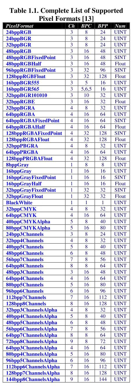
A complete list of currently accepted formats can be seen in Table 1.1 describing the entire list of

different configurations. To synopsize there is support for RGB, Gray, CMYK, black & white,

(21)

[image:21.612.318.545.61.728.2]

9

Table 1.1. Complete List of Supported

Pixel Formats [13]

PixelFormat

Ch

BPC

BPP

Num

24bppRGB

3

8

24

UINT

24bppBGR

3

8

24

UINT

32bppBGR

3

8

24

UINT

48bppRGB

3

16

48

UINT

48bppRGBFixedPoint

3

16

48

SINT

48bppRGBHalf

3

16

48

Float

96bppRGBFixedPoint

3

32

96

SINT

128bppRGBFloat

3

32

128

Float

16bppBGR555

3

5

16

UINT

16bppBGR565

3

5,6,5

16

UINT

32bppBGR101010

3

10

32

UINT

32bppRGBE

3

16

32

Float

32bppBGRA

4

8

32

UINT

64bppRGBA

4

16

64

UINT

64bppRGBAFixedPoint

4

16

64

SINT

64bppRGBAHalf

4

16

64

Float

128bppRGBAFixedPoint

4

32

128

SINT

128bppRGBAFloat

4

32

128

Float

32bppPBGRA

4

8

32

UINT

64bppPRGBA

4

16

64

UINT

128bppPRGBAFloat

4

32

128

Float

8bppGray

1

8

UINT

16bppGray

1

16

UINT

16bppGrayFixedPoint

1

16

SINT

16bppGrayHalf

1

16

Float

32bppGrayFixedPoint

1

32

SINT

32bppGrayFloat

1

32

Float

BlackWhite

1

UINT

32bppCMYK

4

8

32

UINT

64bppCMYK

4

16

64

UINT

40bppCMYKAlpha

5

8

40

UINT

80bppCMYKAlpha

5

16

80

UINT

24bpp3Channels

3

8

24

UINT

32bpp4Channels

4

8

32

UINT

40bpp5Channels

5

8

40

UINT

48bpp6Channels

6

8

48

UINT

56bpp7Channels

7

8

56

UINT

64bpp8Channels

8

64

UINT

48bpp3Channels

3

16

48

UINT

64bpp4Channels

4

16

64

UINT

80bpp5Channels

5

16

80

UINT

96bpp6Channels

6

16

96

UINT

112bpp7Channels

7

16

112

UINT

128bpp8Channels

8

16

128

UINT

32bpp3ChannelsAlpha

4

8

32

UINT

40bpp4ChannelsAlpha

5

8

40

UINT

48bpp5ChannelsAlpha

6

8

48

UINT

56bpp6ChannelsAlpha

7

8

56

UINT

64bpp7ChannelsAlpha

8

64

UINT

72bpp8ChannelsAlpha

9

8

72

UINT

64bpp3ChannelsAlpha

4

16

64

UINT

80bpp4ChannelsAlpha

5

16

80

UINT

96bpp5ChannelsAlpha

6

16

96

UINT

112bpp6ChannelsAlpha

7

16

112

UINT

128bpp7ChannelsAlpha

8

16

128

UINT

(22)

10

1.3.2

Data Hierarchy

Within the HD Photo codec pixel data is grouped into various levels of granularity that are

leveraged throughout. The smallest piece of data is a single pixel coefficient. These coefficients

are then grouped into 4x4 matrix of adjacent values and are referred to as a blocks. Blocks are in

turn regrouped into a 4x4 matrix called a macroblock. The next largest groupings are tiles which

are arbitrary sets of the subdivided image. Tiles can vary in width and height but all tiles in the

same row must have the same height and likewise all tiles in the same column must have the

same width. The largest grouping is the image itself which is extended to fall on macroblock

boundaries. The extension is performed in order to reduce the design logic that would be needed

to handle incomplete macroblocks. An illustration of the spatial hierarchy can viewed in Figure

(23)

[image:23.612.194.417.71.327.2]

11

Figure 1.2. Spatial Layout of Macroblock Aligned Image [13,18]

1.3.3

Frequency Hierarchy

Within the spatial layout the data is orthogonally represented in the frequency domain as well.

As a result of the transform stage the coefficients are grouped into three groups, DC, lowpass

(LP), and highpass (HP). A flow of this process is illustrated in Figure 1.3 and depicts how in

two separate stages one macroblock contains one DC, 15 LP, and 240 HP coefficients. Even

though it might appear that these pixels are then grouped separately, they are in fact still within

(24)

12

Figure 1.3. Process of Developing Frequency Hierarchy

The first stage of the LBT produces one DC coefficient in the top left corner of each block and

the other 15 AC coefficients in the block become the HP band. The second stage of the LBT

operates on the 16 DC coefficients in the macroblock created in the first stage and are operated

on as a block of their own. The DC of the DC coefficients becomes the DC band, 15 AC of DC

coefficients become the LP band, and the rest remain HP coefficients.

1.3.4

Bitstream Structure

A HDP file is arranged so that the beginning set of bytes is dedicated to metadata describing the

rest of the file. This information is followed by an index table that marks where each tile is

located in the bitstream. However each tile may be laid out according to its spatial or frequency

hierarchy, the choice between the two has no real impact on image quality or compression

ability. The only difference is that the frequency hierarchy separates out the data produced as a

result of coefficient normalization that generally has limited information relevant to the quality

(25)

13

Figure 1.4. HD Photo Bitstream Structure [13,15]

1.3.5

Supported Features

One of the benefits of HD Photo is that it can provide both lossy and lossless image compression

using the same algorithm. This is achieved by using a quantization factor of one, which

inherently does not alter the transform data. Other benefits include the use of tiling like that of

JPEG 2000, that enable progressive and ROI decoding. Similarly because of how the

compressed bitstream is structured the encoded image contains its own thumbnail image. HD

Photo also offers support for lossless transcoding operations like flips and rotations on the

compressed image through reordering the macroblocks. A list of the eight supported operations

can be found in Table 1.2.

Table 1.2. Illustration of Combination of Rotate and Flips [15]

Original

Flip

horizontal

Flip

vertical

Flip

horizontal

& vertical

Rotate

90

o

CW

Rotate

90

o

CW

& flip

horizontal

Rotate

90

o

CW

& flip

vertical

(26)

14

2

Design

2.1

Constraints

It is important to note that in an embedded system the image input source is fixed so the

incoming data format is predetermined. For this implementation the pixel format is presumed to

use Blue Green Red (BGR), 8-bit, unsigned integer data. The image size is limited to 11” x 14”

at 600 DPI which is approximately a maximum of 56 megapixels. Reducing the amount of

ambiguity in the design allows for a tighter coupled solution that can improve performance,

shrink the number of logic elements, decrease the amount of test cases, and minimize possible

errors introduced by an elaborate design.

Data streams into the compression algorithm as a series of pixels in raster scan order. The scan

order progresses left to right then top to bottom forming the macroblock aligned image.

Internally all pixel formats are converted so that each image is concurrently represented by a set

of up to 16 color channels, its spatial layout, and its frequency layout. Storing the image like this

provides improved computational flexibility with minimal overhead since the image data size

remains unchanged.

With respect to the color channel representation of the image the first channel is known as the

luma or luminance channel and the rest are chroma or chrominance channels. The number of

chroma channels may vary depending on the color format that is used. In this implementation

(27)

15

responsible for luminance and resembles the monochrome representation of the image. The

chroma channels, U and V, are accountable for the colors in the image. The optional alpha

channel was not applied to add a dimension of transparency to the image.

Each color channel has its own spatial hierarchy and usually has the same resolution but there are

some exceptions. The human eye is more sensitive to the luminance so it is possible to down

sample the chroma channels in lossy modes and reduce the memory footprint while still

maintaining a quality image. For a 4x4 2-D block of pixels on the Y channel, the corresponding

chroma channels may be fully sampled, YUV444, half sampled in the horizontal direction,

YUV422, or half sampled in both the horizontal and vertical direction, YUV420. The YUV444

color space is used in order to keep the data flow and transform components identical for all of

the channels reducing the complexity of the design but requires more logic.

2.2

Image Setup

To simulate an image path data from a BMP bitmap image file must be converted so that it

usable by the rest of the encoder. The data coefficients are read using a Perl script and rewritten

as a series of hex values. The hex values and then able to be read by the testbench at runtime.

(28)

16

The color transform module takes stream of pixel values in BGR sequencing and creates a

macroblock aligned image across the YUV444 color space. As the hex data arrives it must be

immediately converted using Equations 2.1-3. [15]

Color Conversion:

Eqn. 2.1

Eqn. 2.2

Eqn. 2.3

2.4

Lapped Biorthogonal Transform

There are two essential operators used within the LBT, the Photo Core Transform (PCT) and

Photo Overlap Transform (POT). The PCT is comparable to the DCT from the original JPEG

standard in that it exploits spatial locality and has similar drawbacks. However instead of using

an 8x8 matrix of data HD Photo uses a 4x4 matrix. Block transforms are ill-suited for taking

advantage of redundancy across block boundaries resulting in possible blocking artifacts in the

compressed image. The POT was designed to help mitigate this drawback by operating on data

(29)

17

optional. The POT has three different configurations, on for both, off for both, or on for only the

first stage. The quality and performance requirements can dictate how the POT needs to

supported, possibly reducing the size and complexity. For this design the POT will be on for

both stages to achieve the best image quality.

Figure 2.1. PCT and POT Operation Boundaries [14]

One of the main implementation issues of the compression algorithm is the tradeoff between

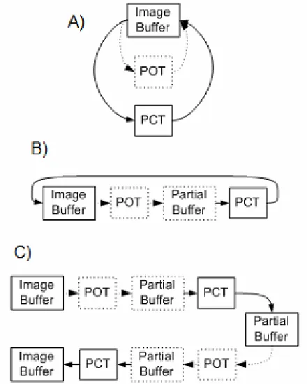
maintaining a small memory footprint and a fully pipelined design. Images can be of significant

size and increasing the image buffers within design can be proportionally related to the size and

throughput of the design. Figure 2.2 presents three different approaches for implementing the

(30)

[image:30.612.196.416.71.346.2]

18

Figure 2.2. Various LBT Implementation Techniques

Figure 2.2A demonstrates how one image buffer can drive and store data to and from the

appropriate transform(s). This approach uses the least amount of memory, but requires either

each transform to complete one at a time or a fairly sophisticated image buffer to continually

load and store sets of data. Figure 2.2B uses an intermediary partial image buffer that allows the

coefficients to enter the PCT directly from the POT. The advantage to using the partial buffer is

an improved pipeline architecture that does not require the space of a second full image buffer.

If no POT is applied at either stage then the two implementations are identical. This design

however implements an approach that resembles Figure 2.2C which is a fully pipelined and will

yield the highest throughput and largest memory footprint. Like Figure 2.2B, partial buffers are

used in between the transform gaps. Once all the data is loaded into the first transform the

(31)

19

2.4.1

Photo Core Transform

The PCT itself is comprised of several smaller transforms because a separable 2-D transform can

be implemented by performing 1-D transforms on the rows of data in conjunction with a 1-D

transforms on the columns of data.

2.4.1.1

2x2 Hadamard Transform

The Hadamard transform is a 2-point operator that can mathematically be described by equation

2.4. The 2x2 Hadamard transform is developed by taking the Kronecker product of the 2-point

Hadamard with itself as seen in equation 2.5 [13].

Eqn. 2.4

Eqn. 2.5

The math is then reduced to a series of trivial lifting steps described in pseudo-code in Figure

(32)

20

2x2T_h (a,b,c,d, R) {

int t1, t2

a += d

b –= c

t1 = ((a – b + R) >> 1)

t2 = c

c = t1 – d

d = t1 – t2

a –= d

b += c

[image:32.612.231.381.68.235.2]

}

Figure 2.3. Pseudo-code for 2x2 Hadamard Transform [13]

2.4.1.2

2x2 Odd Transform

The odd transform was developed by taking the Kronecker product of a 2-point rotation operator

described in equation 2.6 and the 2-point Hadamard operator [13].

Eqn. 2.6

The transform can be reduced to a set of equations including four that are non-trivial as described

by the pseudo-code found in

(33)

21

T_odd (a,b,c,d) {

b –= c;

a += d;

c += ((b + 1) >> 1);

d = ((a + 1) >> 1) – d;

b –= ((3*a + 4) >> 3);

a += ((3*b + 4) >> 3);

d –= ((3*c + 4) >> 3);

c += ((3*d + 4) >> 3);

d += (b >> 1);

c –= ((a + 1) >> 1);

b –= d;

[image:33.612.220.394.67.295.2]

a += c;

}

Figure 2.4. Pseudo-code for 2x2 Odd Transform [13]

2.4.1.3

2x2 Odd-Odd Transform

The odd-odd transform was developed by taking the Kronecker product of a 2-point rotation

operator with itself. The transform can be reduced to a set of equations including three that are

(34)

22

T_odd_odd (a,b,c,d) {

int t1, t2;

b = –b;

c = –c;

d += a;

c –= b;

a –= (t1 = d >> 1);

b += (t2 = c >> 1);

a += ((b * 3 + 4) >> 3);

b –= ((a * 3 + 3) >> 2);

a += ((b * 3 + 3) >> 3);

[image:34.612.213.401.66.337.2]

b –= t2;

a += t1;

c += b;

d –= a;

}

Figure 2.5. Pseudo-code for 2x2 Odd-Odd Transform [13]

2.4.1.4

4x4 Photo Core Transform

The PCT itself is a series of Hadamard, odd, and odd-odd transforms. The order and data flow

can be found in the pseudo code of Figure 2.6. In total each PCT contains 15 non-trivial

operations. The set of transforms used can logically be broken up to occur in two separate stages

(35)

23

4x4PCT (Coeff[0], …, Coeff[15]) {

// First stage

2x2T_h(Coeff[0], Coeff[3], Coeff[12], Coeff[15], 0)

2x2T_h(Coeff[5], Coeff[6], Coeff[9], Coeff[10] , 0)

// Second stage

2x2T_h(Coeff[0], Coeff[1], Coeff[4], Coeff[5], 1)

T_odd(Coeff[2], Coeff[3], Coeff[6], Coeff[7])

T_odd(Coeff[8], Coeff[12], Coeff[9], Coeff[13])

T_odd_odd(Coeff[10], Coeff[11], Coeff[14], Coeff[15])

// Permute the coefficients

FwdPermute(Coeff[0], Coeff[1], …, Coeff[15])

}

Figure 2.6. Pseudo-code for 4x4 PCT [13]

2.4.2

Photo Overlap Transform

The POT uses some of the same transforms as the PCT but includes another two. These two are

the 2-point rotation and the 2-point scaling operations. Since the POT operates across

macroblock boundaries edge cases are created that require the use of a 4-point transform along

with a 4x4 transform.

2.4.2.1

2-Point Rotation

The rotate transform can be found in equation 2.6 and is demonstrated in pseudo-code with three

(36)

24

fwdRotate (a,b) {

a += ((b * 3 + 8) >> 4);

b –= ((a * 3 + 4) >> 3);

a += ((b * 3 + 8) >> 4);

[image:36.612.232.380.69.145.2]

}

Figure 2.7. Pseudo-code for 2-Point Rotation Transform [13]

2.4.2.2

2-Point Scaling

The scaling function is a result of the matrix that can be found in equation 2.7 [13]. It can be

remapped as the pseudo-code with three non-trivial functions found in Figure 2.8.

Eqn. 2.7

fwdScale (a,b) {

b += a;

a –= ((b + 1) >> 1);

b –= ((a * 3 + 4) >> 3);

a –= ((b * 3 + 8) >> 4);

b –= ((a * 3 + 0) >> 3);

a += ((b + 1) >> 1);

b –= a;

}

[image:36.612.234.376.349.617.2]

(37)

25

2.4.2.3

4-Point Overlap Transform

At both stages there is a ring of coefficients two thick that the 4x4 POT cannot be applied to.

The 2x2 matrix of coefficients formed at each corner are passed through while the rest of the

border is grouped into 2x4 blocks and fed through two of the 4-point POT. The pseudo-code

describing the 4-point POT containing nine non-trivial operations can be found in Figure 2.9.

4PreFilter (a,b,c,d) {

a –= ((d * 3 + 16) >> 5);

b –= ((c * 3 + 16) >> 5);

d –= ((a * 3 + 8) >> 4);

c –= ((b * 3 + 8) >> 4);

a += d – ((d * 3 + 16) >> 5);

b += c – ((c * 3 + 16) >> 5);

d –= ((a + 1) >> 1);

c –= ((b + 1) >> 1);

fwdRotate(c, d);

d += ((a + 1) >> 1);

c += ((b + 1) >> 1);

a –= d;

b –= c;

[image:37.612.218.397.269.528.2]

}

Figure 2.9. Pseudo-code for 4-Point POT [13]

2.4.2.4

4x4 Photo Overlap Transform

The POT like the PCT is a series of smaller transforms with 27 non-trivial operations. Logically

the flow of transforms can be separated into four different pipelined stages. The pseudo code

(38)

26

4x4PreFilter (a,b,...,p) {

2x2T_h(a, d, m, p, 0);

2x2T_h (b, c, n, o, 0);

2x2T_h (e, h, i, l, 0);

2x2T_h (f, g, j, k, 0);

fwdScale (a, p);

fwdScale (b, l);

fwdScale (e, o);

fwdScale (f, k);

fwdRotate (n, m);

fwdRotate (j, i);

fwdRotate (h, d);

fwdRotate (g, c);

T_odd_odd (k, l, o, p);

2x2T_h (a, m, d, p, 0);

2x2T_h (b, n, c, o, 0);

2x2T_h (e, i, h, l, 0);

2x2T_h (f, j, g, k, 0);

[image:38.612.228.384.64.402.2]

}

Figure 2.10. Pseudo-code for 4x4 POT [13]

2.5

Quantization

Quantization is one of the key stages in terms of compressing the image. The QP can be varied

over the three orthogonal representations of the image. Each color plane may have the same QP,

the luma and chroma channels may have separate QP, or each channel may have an individual

QP. In the spatial domain every tile may have the same QP, each tile may have a unique QP, or

there can be 16 different QP for macroblocks within a tile. In the frequency domain each band

may use the same QP, the LP and HP can use separate QP from the DC band, the DC and LP can

(39)

27

harmonic quant values which are applied to divide down the image coefficients reducing their bit

sizes. In lossless encoding a quant value of one is used.

If lossless compression is required then quantization may be left out of the design all together.

However for this design a set of registers are implemented to track the QP values and settings,

and parallel dividers are used for each color channel.

2.6

Adaptive Coefficient Prediction

The coefficient prediction stage is designed to remove inter-block redundancy in the quantized

transform coefficients while minimizing the storage requirements. The prediction scheme

however is only used when the inter-block correlation has a strong and dominant orientation

[15]. DC and LP prediction occurs across macroblock boundaries, but HP prediction happens

within a macroblock. Prediction uses adjacent pixel coefficients with the same QP to determine

if there is a dominant prediction direction that determines which if any coefficients should be

updated. The DC band uses its top, left, and top left DC neighbors as illustrated in Figure 2.11,

where D represents the top-left coefficient (diagonal), T is the top, L is left, and X is the

(40)

28

X

T

L

D

X

T L D

X T L D

luminance

[image:40.612.248.366.474.596.2]

chrominance

Figure 2.11. DC Prediction Layout [15]

The LP band determines its prediction direction based off of the DC prediction direction. And

the HP band uses the LP coefficients to determine its prediction direction. Predicted values are

derived from the same band coefficients that are adjacent row above or column to the left of the

current macroblock or block in the HP band’s case. Eventually the predicted values are added to

the current macroblock coefficients based on the direction predictor. The LP coefficients either

use three coefficients from the top row of a macroblock or three coefficients from the leftmost

column as highlighted in Figure 2.12.

Figure 2.12. LP Coefficient Prediction [15]

The HP predicted values used are similar to the LP prediction scheme in the top row or left

column is used to predict. A visual depiction of left prediction can be found in Figure 2.13, but

(41)

[image:41.612.157.455.97.405.2]

29

Figure 2.13. HP Left Prediction Scheme [14,15]

Because the HP direction is based off of the LP coefficient and the LP direction is determined by

the DC direction there are dependencies between the three bands so they must occur in a specific

order. This design predicts for one block at a time so each DC and six of the LP coefficient

values must be stored for prediction of future blocks as data flows through the pipeline. Since

HP prediction does not cross macroblock boundaries 36 coefficients need to be stored but can be

dumped at the next macroblock.

(42)

30

Scanning is the process of converting the 2-D matrix of coefficients into a 1-D array so that it

may be encoded. The DC coefficients are ordered in raster scan order while the LP and HP

coefficients must be ordered in some manner. In JPEG traditionally known as zigzag scanning,

HD Photo uses two different scan orders depending on the prediction direction and a statistical

[image:42.612.226.385.236.319.2]

average can modify those orders. The initial orders are displayed in Figure 2.14.

Figure 2.14. Initial Scan Patterns (a) LP and HP Horizontal (b) HP Vertical [15]

As values are scanned a tally of the non-zero coefficients are kept in order to predict future

clusters of zero coefficients. By adjusting the scan order to a more favorable bit stream the

overall number of bits in the compressed image can be decreased by an average of 3%. The scan

order can be determined independent from neighboring macroblocks and therefore directly

pipelined with the prediction stage as blocks of coefficients become available. An example of an

adjustment to the scan order is illustrated in Figure 2.15. Figure 2.15a shows that box 5 has

more non-zero coefficients than box 8, so in Figure 2.15b the two boxes are switched in the

(43)

31

Figure 2.15. Example of Adaptive Coefficient Scanning [15]

2.8

Adaptive Entropy Encoding

The HD Photo compression algorithm uses a 3½D - 2½D coding approach that in contrast to 2D

or 3D coding tracks the number of zeros trailing a non-zero coefficient in the bit stream. The

first non-zero coefficient must signal both the run of zeros preceding and trailing in the bit

stream for this encoding to work. An example stream with five symbols is found in Figure 2.16.

Figure 2.16. Example 3½D - 2½D Coded Stream [15]

For all of the symbols the trailing run can be zero, non-zero, or the last coefficient and the level

can be one or greater. Therefore to encode the basic 2 ½D symbol the language is limited to a

(44)

32

language required to encode these symbols is twice as large meaning a code of 12. The

coefficient levels and signs are encoded according to their frequency band and use the VLC

tables to translate the resulting bitstream. There are seven adaptable predefined VLC tables used

to translate the bitstream as shown in Figure 2.17.

Figure 2.17. VLC Coding Tables used by HD Photo [13,14,15]

Each table is designed for a closed language with a different number of symbols per table. Some

tables describe more than one translation code per language. A set of weighted estimations are

monitored so the encoding algorithms can switch to a more desirable code within a table at run

time. The use of small predefined VLC tables helps maintain a small memory footprint and the

estimation algorithm is computationally light. Since encoding is macroblock independent

(45)

33

2.9

Adaptive Coefficient Normalization

In order to produce better suited coefficients for the 3½D - 2½D encoding procedure only the 12

MSB of each LP coefficient and eight MSB for the HP coefficients are used to determine the

level. The four LSB of the LP and eight LSB of the HP are left unaltered and grouped into what

are referred to as flexbits including a sign indication. The nature of the LP and HP bands makes

this data of limited importance and may be discarded in lossy compression if so desired. A

simple picture of how this process takes place is captured in Figure 2.18

(46)

34

3

Implementation

3.1

Lapped Biorthogonal Transform

3.1.1

General Transform Information

Within all the transforms the non-trivial steps are multiplies in the form of

_n

2

3

with some

rounding correction. Luckily all of these non-trivial operations can be reduced to a simpler set of

additions and shifting without the use of a multiplier or divider. This can be done by dividing

the calculation into smaller pieces and then pipelining the results together. First to obtain a

multiply by three, feed an adder the same number on both input ports, with one input left shifted

by one bit. The left shift has the same effect as a multiply of two without the added LUTs or

dedicated DSP blocks inside the FPGA. The rounding correction is usually half the value of the

denominator, and is added on so that when division occurs the result is not always rounded

down. Lastly and most importantly since all the divisions are 2

n,

they can be achieved through a

right shift. There is only some small Boolean check to make sure the sign of the value remains

intact. Because this solution is implemented on a FPGA that uses LUTs instead of normal gates

it tends to be more efficient to use the default macros included in the Quartus II MegaWizard for

(47)

35

3.1.2

Photo Core Transform

3.1.2.1

2x2 Hadamard Transform

The implementation of the Hadamard transform can be seen in Figure 3.1 and contains only

trivial operations of which are divided into six pipelined stages. In total there are eight instances

[image:47.612.107.508.322.531.2]

of addition / subtraction.

Figure 3.1. Structural Overview of 2x2 Hadamard Transform

(48)

36

The implementation of the Odd transform can be seen in Figure 3.2 and contains only trivial

operations of which are divided into 16 pipelined stages. In total there are 24 instances of

addition / subtraction.

Figure 3.2. Structural Overview of 2x2 Odd Transform

3.1.2.3

2x2 Odd-Odd Transform

The implementation of the Odd-Odd transform can be seen in Figure 3.3 and contains only trivial

addition / subtraction.

(49)

37

3.1.2.4

4x4 Photo Core Transform

The implementation of the PCT transform can be seen in Figure 3.4 and contains only trivial

addition / subtraction. In order to produce results concurrently extra registers needed to be added

into the pipeline before the second set of transforms.

Hadamard

A_in

B_in

C_in

D_in

E_in

F_in

G_in

H_in

I_in

J_in

K_in

L_in

M_in

N_in

O_in

P_in

Hadamard

Odd

Odd Odd

REG 12x

REG 12x REG 12x REG 12x

REG 2x

A_out

B_out

C_out

D_out

E_out

F_out

G_out

H_out

I_out

J_out

K_out

L_out

M_out

N_out

O_out

[image:49.612.123.493.270.671.2]

P_out

(50)

38

3.1.3

Photo Overlap Transform

3.1.3.1

2-Point Rotation

The implementation of the rotation transform can be seen in Figure 3.5 and contains only trivial

operations of which are divided into 12 pipelined stages. In total there are nine instances of

Figure 3.5. Structural Overview of 2-Point Rotation

3.1.3.2

2-Point Scaling

The implementation of the scaling transform can be seen in Figure 3.6 and contains only trivial

(51)

39

3.1.3.3

4-Point Overlap Transform

The implementation of the 4-point POT transform can be seen in Figure 3.7 and contains only

trivial operations of which are divided into 31 pipelined stages and 17 buffer registers at the

output to align with the 4x4 POT. In total there are 39 instances of addition / subtraction.

[image:51.612.73.524.259.492.2]

A_in B_in C_in D_in REG REG REG REG REG REG REG REG REG REG REG REG REG REG REG REG REG

+

>>

4 REG REG REG REG

+

<<1 REG REG REG REG REG REG REG

+

>>

5 REG REG REG REG

+

REG

>>

5

>>

5 <<1

–

REG REG

–

<<1 REG REG REG REG REG REG REG REG

+

>>

1 REG

+

<<1

+

REG REG REG REG

+

16'h10

+

–

+

16'h8

>>

4

+

<<1 REG

–

+

16'h10

>>

5

+

<<1

+

–

+

16'h1

>>

1 REG

–

REG REG REG REG REG REG REG REG

+

16'h8

>>

4 REG REG REG REG

+

<<1 REG REG REG

+

16'h4

>>

3 REG REG REG REG

+

<<1 REG REG REG

–

+

16'h8

>>

4 REG REG REG REG

+

<<1 REG REG REG

+

>>

1

+

16'h1

>>

1 REG REG

+

REG REG

–

REG x 17 REG x 17 REG x 17 REG x 17 A_out B_out C_out D_out

Figure 3.7. Structural Overview of 4-Point POT

3.1.3.4

4x4 Photo Overlap Transform

The implementation of the 4x4 POT can be seen in Figure 3.8 and contains only trivial

addition / subtraction. The design is grouped into four stages in which buffers needed to be

(52)

40

Hadamard A_in

B_in

C_in D_in

E_in

F_in

G_in H_in

I_in

J_in

K_in L_in M_in

N_in

O_in P_in

Hadamard

A_out

M_out

B_out

N_out D_out

P_out

C_out

O_out

E_out

I_out

F_out

J_out H_out

L_out

G_out

K_out

Odd Odd

Hadamard

Hadamard REG 18x

REG 18x

REG 18x REG 18x REG 18x Scale

Scale

Rotate

Rotate REG 8x

REG 8x

REG 8x REG 8x

REG 8x

[image:52.612.87.527.87.401.2]

REG 8x REG 8x

Figure 3.8. Structural Overview of 4x4 POT

3.1.4

16x16 Lapped Biorthogonal Transform

The implementation of the LBT can be seen in Figure 3.9 and contains only trivial operations of

which are divided into 111 pipelined stages. In total there are 640 instances of addition /

subtraction. In order to fully exploit the parallelism that exists within the design two 4-point

POT are used in parallel with one 4x4 POT and a pass through buffer for the corner coefficients.

In order to start producing complete blocks of coefficients at a time without buffering

(53)

41

a single pass though it were a 5x5 block. The data that pertains to other blocks will be

recalculated later when it is the turn for that block to undergo the POT. The results from the first

stage POT transforms are input into 16 orthogonal 16-bit 6,608 column by 4 row RAM structures

one for each position in the macroblock so data can be entered and retrieved in parallel while

making sure that all calculated data is preserved until it is no longer needed. Once enough of the

POT values have been calculated the first stage PCT is signaled it can start. As data comes out of

the PCT transform there are 15 HP coefficients per block generated that are stored into 15

orthogonal 16-bit 6,608 column by 4 row RAM structures and wait for the DC and LP values to

finish being calculated. The DC/LP coefficients are fed into a separate set of 16-bit 413 column

by 4 row RAM structures that are used to supply the second stage POT with data. Following a

similar process at a different granularity level the second stage POT and PCT produce the DC

and LP coefficients which are then realigned with their corresponding block of HP coefficients

(54)

[image:54.612.137.477.69.673.2]

42

(55)

43

3.2

Quantization

The quantization stage is fairly straightforward and is composed of two components, a 4x4

quantizer and a quant map. Together the two components store the quantization settings

including all of the different QP associated with the setting and a ten clock divider to apply the

quant values.

3.2.1

Quant Map

The quant map takes in the user specified QP and stores them according to the quantization

settings selected by the user. As requests for specific blocks come in the QP are sent out to the

(56)

[image:56.612.109.504.70.359.2]

44

Figure 3.10. Structural Overview of Quant Map

3.2.2

4x4 Quantizer

The 4x4 quantizer is signaled by the LBT that the data stream is ready, at which point the control

logic starts to iterate over the block data, requesting specific QP. When the QP are retrieved from

the map they are converted into their quant values and then applied using a 10 clock cycle

(57)

[image:57.612.134.474.76.417.2]

45

Figure 3.11. Structural Overview of 4x4 Quantizer

3.3

Adaptive Coefficient Prediction

An overview of how the adaptive prediction stage was designed can be found in Figure 3.12.

The macroblock flows in block by block in raster scan order. The zeroth block contains the DC

values so they are used along with the stored DC top-left, top, and left neighbors to determine the

DC and LP predict direction. Knowing the DC direction its value can immediately be predicted

and wait until it is needed at the output. The LP prediction direction might be left so the LP

(58)

46

in. At this point the LP Direction can dictate how to predict the LP values and the HP predict

direction can be calculated. The HP values must be buffered up until the fifteenth and final block

arrives at which point the HP values can be predicted. At the output some control logic realigns

the frequency bands and sends the valid data out block by block.

y_0

y_4

y_8

y_1

u_1

u_8

u_12

u_2

u_3

v_0

v_1

u_4

y_2

y_12

u_0

y_3

y_out

u_out

v_out

v_8

v_12

v_2

v_3

v_4

data_in_valid

mblock_height

mblock_width

Control

Logic

y_in

u_in

v_in

DC Predict

Direction

LP Buffer

HP Buffer

DC Predict

DC

Storage

LP Predict

LP Storage

HP Predict

Direction

Control

Logic

[image:58.612.85.527.217.676.2]

hp_vertical_scan

data_out_valid

(59)

Modeling and synthesis of the HD photo compression algorithm

Rochester Institute of Technology

in Theses by an authorized administrator of RIT Scholar Works. For more information, please contact

Committee Member

I, Seth

Abstract

HD Photo was chosen to become the next JPEG standard because it has a computationally light

transform. HD Photo also has adaptive coefficient prediction and scanning stages to help furnish

HD Photo and the current JPEG standard using the HD Photo plug-in for Adobe’s Photoshop

The author would like to acknowledge all of the direction, guidance, and assistance he has

Table of Contents

Bitstream Structure ... 12

General Transform Information... 34

Layout Analysis ... 55

Appendix C. Perl Script ... 100

Figure 1.3. Process of Developing Frequency Hierarchy ... 12

Figure 2.6. Pseudo-code for 4x4 PCT [13] ... 23

Figure 2.13. HP Left Prediction Scheme [14,15]... 29

Figure 3.3. Structural Overview of 2x2 Odd-Odd Transform ... 36

Figure 3.11. Structural Overview of 4x4 Quantizer ... 45

Figure 5.1. Chart of Compression Time vs. Amount of Pixels in the Image... 57

Glossary

encoding process.

image contains meaningful data.

and memory.

High Dynamic Range – Term used to describe pixel formats that can represent a

produced by the group.

data co-located across all color channels

across block boundaries to reduce blocking artifacts within the compressed

compressed bitstream.

, y, and two

channel is a 4x4 matrix of pixel

handle new high dynamic range (HDR) and wide gamut formats because their algorithms were

format spectrum while still remaining computationally efficient and portable.

was under

Currently Microsoft’s HD Photo is in the review process of becoming the newest JPEG standard

constrain the design to implement only the necessary components of the algorithm while still

design to obtain timing, power, and gate count information.

was verified for functionality and operation. The fifth chapter presents the results achieved by

the BMP into a HEX file is located in Appendix C. Finally the synthesis reports generated by

On the other hand lossy image codecs take advantage of the fact that some visual data is

sample size. For instance taking pixel coefficients into a domain that can exploit the samples’

image compression the data that falls into the invisible or barely visible spatial frequencies may

each pixel to be represented by fewer bits, but the quantization factor used can have a great

compression there are a handful of techniques to reduce the bitstream that can be leveraged by

events requiring a longer code than their original fixed length. Another popular technique is run

Current Digital Still Image Codecs

become ubiquitous within the digital continuous tone still image field. JPEG sees use in a wide

The despite the widespread support of JPEG there are several limitations. Newer pixel formats,

compressed image file cannot produce its own thumbnail or be progressively decoded.

be independently decoded. Independent data groupings provide the ability to randomly access

gained widespread support from web browsers and embedded applications like digital cameras.

in Figure 1.1 at a high level HD Photo is quite similar to the JPEG standard but there is quite a

factor. HD photo on the other hand has three settings for the transformation stage that can be

keeps a statistical measure for which variable length coding (VLC) table is used and switches to

data can differ in numerical format, number of color channels, organization of color channels,

option due to clipping that will occur somewhere within the algorithm.

A complete list of currently accepted formats can be seen in Table 1.1 describing the entire list of

48bppRGBHalf

8bppGray

56bpp7Channels

56bpp6ChannelsAlpha

leveraged throughout. The smallest piece of data is a single pixel coefficient. These coefficients

same width. The largest grouping is the image itself which is extended to fall on macroblock

As a result of the transform stage the coefficients are grouped into three groups, DC, lowpass

Figure 1.3. Process of Developing Frequency Hierarchy

coefficients become the LP band, and the rest remain HP coefficients.

hierarchy, the choice between the two has no real impact on image quality or compression

using the same algorithm. This is achieved by using a quantization factor of one, which

compressed image through reordering the macroblocks. A list of the eight supported operations

incoming data format is predetermined. For this implementation the pixel format is presumed to

errors introduced by an elaborate design.

provides improved computational flexibility with minimal overhead since the image data size

responsible for luminance and resembles the monochrome representation of the image. The

sample the chroma channels in lossy modes and reduce the memory footprint while still

the channels reducing the complexity of the design but requires more logic.

The color transform module takes stream of pixel values in BGR sequencing and creates a

Photo Overlap Transform (POT). The PCT is comparable to the DCT from the original JPEG

optional. The POT has three different configurations, on for both, off for both, or on for only the

One of the main implementation issues of the compression algorithm is the tradeoff between