Detecting Common Longevity Trends by a Multiple Population Approach

City, University of London Institutional Repository

Citation

:

Detecting Common Longevity Trends by a Multiple Population Approach. North American Actuarial Journal, 18(1), pp. 139-149. doi: 10.1080/10920277.2013.875884

This is the accepted version of the paper.

This version of the publication may differ from the final published

version.

Permanent repository link:

Link to published version

:

Copyright and reuse:

City Research Online aims to make research

outputs of City, University of London available to a wider audience.

Copyright and Moral Rights remain with the author(s) and/or copyright

holders. URLs from City Research Online may be freely distributed and

linked to.

City Research Online: http://openaccess.city.ac.uk/ [email protected]

Detecting longevity common trends by a multiple population approach

Valeria D’Amato1, Steven Haberman2,Gabriella Piscopo3, Maria Russolillo1, Lorenzo Trapani4

1 _{Department of Economics and Statistics, University of Salerno, via Ponte Don Melillo, Campus}

Universitario, 84084 Fisciano (Salerno), Italy

e-mail: [email protected], [email protected]

2 _{Faculty of Actuarial Science and Insurance, Cass Business School, City University, Bunhill Row}

London, UK, e-mail: [email protected],

3 _{Department of Economics, University of Genoa, Via Vivaldi, 16126 Genoa, Italy - e-mail:}

[email protected]

4 _{Faculty of Finance, Cass Business School, City University, Bunhill Row London, UK, e-mail:}

[email protected]

Abstract. Recently the interest in the development of country and age-based longevity risk models (Njienga and Sherris. 2011) has been growing. The investigation of long-run equilibrium relationships could provide valuable information about the factors driving changes in mortality, in particular across ages and across countries.

In order to investigate cross-country longevity common trends, tools to quantify, compare and model the strength of dependence become essential. On one hand it is necessary to take into account either the dependence for adjacent age groups, or the dependence structure across time in a single population setting: a sort of intra-dependence structure (D’Amato et al. 2012b). On the other hand, the dependence across multiple populations, which we describe as inter-dependence, can be explored for capturing common long run relationships between countries. In particular, the objective of our work is to produce longevity projections by taking into account the presence of various forms of cross-sectional and temporal dependencies in the error processes of multiple populations, considering mortality data from different countries. The algorithm that we propose combines model-based predictions in the Lee Carter framework (1992) with a bootstrap procedure for dependent data, and so both the historical parametric structure and the intra-group error correlation structure are preserved. We modify the model presented by D’Amato et al. (2012b), which applies a sieve bootstrap to the residuals of the Lee Carter model. According to this scheme, they are able to reproduce in the sampling the dependence structure of the data under consideration. In this paper, the algorithm we build is performed on a pool of populations by using ides from panel data; we refer to this new algorithm as the Multiple Lee Carter Panel Sieve (MLCPS). By considering a group of associated populations that have similar socioeconomic conditions, we are interested in estimating the relationships between them, and identifying the common features in the group. The empirical results show that the MLCPS approach works well in the presence of dependence.

Keywords: Serial and Cross-sectional Correlation, Factor Models, Vector

AutoRegression, Sieve Bootstrap, Lee Carter model

1. Introduction

In the actuarial literature and practice, the interest in the development of country and age-based longevity risk models is increasing (Njienga and Sherris. 2011). Attention is focused on investigating long-run equilibrium relationships and collecting valuable information about the factors driving the changes in mortality, in particular across ages and countries. The importance of considering a synoptic approach has been highlighted by Li and Lee (2005). They show improvement of the mortality projections for individual countries by taking into account the

patterns in a larger group. Thus, Tuljapurkar et al (2000)identify a ‘universal pattern’ of mortality

model, Russolillo et al. (2011)provide an aggregate estimate for a set of countries. The underlying idea is to produce projected life tables for the set of countries under consideration.

Lazar and Denuit (2009) extract and forecast the common stochastic trends shared by the time series of log-death rates, where the common factors can be modelled as a multivariate random walk with drift. To hedge against the basis risk, Li and Hardy (2011) connect the longevity improvements of two different populations by the Augmented Common Factor Model in the Lee Carter setting. They show that using two independent Lee-Carter models is likely to result in an increasing divergence in life expectancy in the long run. This is counter to a global convergence in mortality

levels, as documented in White (2002), Wilson (2001), and United Nations (1998).

In order to investigate cross-country longevity common trends, we adopt a multiple population

approach. For the purposes under consideration, the dependence structure has to be taken into

account, to avoid an underestimation of the actual mortality risk. Indeed, the pressing need of the correct representation of the longevity phenomenon is also more relevant in light of the new regulatory guidelines prescribed by Solvency II. In order to produce accurate longevity projections, it is essential to include the so-called dependency risk, which is a significant source of risk as

explained in D’Amato et al. (2011). On one hand it is necessary to take into account either the

dependence for adjacent age groups, or the dependence structure across time for a single population: which is a type of intra-dependence. On the other hand, the dependence across the multiple populations under consideration has to be explored: here we describe this as inter-dependence.

The existence of dependence in mortality data involves the interactions between age and time. In

particular, the mortality experience of countries in the industrialized world over the course of the twentieth century would suggest a substantial age-time interaction: two dominant trends have

affected different age groups at different times. Booth et al. (2002)show that the interaction exists,

in the application of the Lee-Carter (henceforth LC) model to Australian data. Furthermore, they

acknowledge that the main methodological problem in the LC model is the assumption of invariance in the age component. To overcome the problem they propose an extension of the

original nature of the model. According to other authors, like Stevens (2011), the assumption that

bx component in LC is time-independent is violated. In fact, empirical evidence shows that this

assumption is violated. In particular, Stevens proposes a different variant to the traditional Lee Carter model, as a time-dependent-age factor. Others have introduced switching regimes (Hainut, 2012) or multiple factor models for mortality using an affine model for all ages simultaneously (Gaille et al. 2011). In particular, a multiple Lee Carter model is developed to capture the stochastic trends in mortality improvements at different ages and across time as well as a multivariate dependence structure across ages.

In this paper, we consider a different approach to the issue of cross-sectional and time dependence. We retain the parametric structure of the LC model, but we extend the basic framework to include some cross dependence in the error term. As far as time dependence is concerned, we allow for all idiosyncratic components (both in the common stochastic trend and in the error term) to follow a linear process, thus considering a highly flexible specification for the serial dependence structure of our data. We also relax the assumption of normality, which is typical of early studies on mortality (Lee and Carter, 1991) and on factor models (see e.g. the textbook by Anderson, 1984). Whilst the technical details are in Section 4, we point out that our model nests the standard LC framework, thereby having the same properties and also being more general.

method) may be flawed in small samples; moreover, limiting distributions of estimated parameters depend upon several nuisance parameters whose estimation can be fraught with difficulties. Thus, the bootstrap can be, in this context, a valid alternative. By virtue of our assumption on the time dependence structure, we apply a sieve bootstrap algorithm (Bulhmann, 1997) to the Vector AutoRegression (VAR henceforth) model containing the estimated common factors (both stationary and nonstationary). However, in our context we cannot apply a standard sieve bootstrap algorithm, since, when resampling the estimated common factors, a generated regressors problem arises. Trapani (2012) develops the full blown theory to apply sieve bootstrap to the context of nonstationary panel factor series, developing selection rules for the order of the VAR and showing the superior performance of sieve bootstrap compared to first-order asymptotics. Our paper is therefore the first application of the bootstrap theory for nonstationary panel factor series.

Based on this methodology, we produce longevity projections by taking into account the presence of various forms of cross-sectional and temporal dependencies in the error processes in related to a multiple population dataset, composed of mortality data from different countries. The benefit of the

aforementioned framework is twofold. It “replicates” the mortality of the small population by

mixing appropriately the mortality data from neighbouring countries, as suggested in Olivieri (2011). Some recent contributions reveal the importance of this aspect. Thus, Cairns et al (2011) represent the joint development over time of mortality rates in a pair of related populations. Jarner and Kryger (2009) introduce a proposal for robust forecasting based on the existence of a larger reference population.

Furthermore, our approach is intended to avoid a problem leading to inconsistent estimates due to misleading inference and even inconsistent estimators.

The remainder of the paper is organised as follows. Section 2 introduces the LC model. In section 3, we present the setting of multiple population on which we develop the algorithm. Section 4 is devoted to the Multiple Lee Carter Panel Sieve that we propose. Section 5 shows the numerical applications. Finally, section 6 concludes.

2. Demographic scenario: the Lee Carter model

Lee and Carter (1992) suggested a log-bilinear form for the force of mortality:

)

exp( _{x x t xt}

xt k u

m    

 

xt t x x xt

xt m k u

y ln( )  

 

describing the log of a time series of age-specific death rates m_xt as the sum of an age-specific

parameter independent of time _xand a component given by the product of a time-varying

parameter k_t, reflecting the general level of mortality and the parameter _x, representing how

rapidly or slowly mortality at each age varies when the general level of mortality changes.

We refer to Lee and Carter (1992) for a fuller discussion of the model.

In this research we analyse mortality datasets related to five populations experiencing common

longevity improvements, in order to compare the survival evolution in different countries in the

light of cross-country common trends. Working with different populations, the dependence structure analyzed in previous works for a single dataset (D’Amato et al. 2012a) becomes very complex and has to be taken into account under a multidimensional approach. In fact, the cross sectional dependence for adjacent age groups, across countries and serial/time dependence have to

be considered. In this case, the classical VAR sieve bootstrap framework appears infeasible and

cannot be applied to our three-dimensional dataset, because the number of cross-sectional units is too large. Thus, we present an original contribution to overcome the problem of analyzing dependence in the case of multiple populations.

Our research starts from the idea that the common trends between countries are captured by the

parameters k_t of the Lee Carter model. For this reason, we fit separately the Lee Carter on some

mortality dataset of M different populations, composed by the same ages xa a, 1, ,aN and

years tb b, 1, ,b T , where a represents the first age and b the first time, respectively. Once

we have obtained the kt’s for each country, we arrange the M time series of kt in a matrix,

generating a panel data in which the single units are represented by the different populations and are collected in rows. As it is clear, the approach is completely different from the previous one: in the case of one population, each single unit is represented by a different age; the variable observed is

the central mortality death rate and the observations are NT , consisting of time series of length T,

on N _{parallel units-ages. Instead, in the case of multiple populations, each single unit is}

represented by a different population; the variable observed is the parameter kt of that particular

population, which is able to explain the mortality trend; thus the observation are MT, consisting of

M _{time series of length} T, one for each population. On this reduced dataset, it is possible to

implement the VAR _{sieve scheme.}

4. Algorithm: Multiple Lee Carter Panel Sieve

This section discusses the methodology to generate the bootstrap sample. Consider (2), and define

, 1

k t t

t k e

k  _ 

where ekt is a stationary process. Detailed assumptions on the form of serial dependence in kt and uxt

are in Trapani (2012).

Prior to explaining the actual bootstrap algorithm, there in (2) it is necessary to estimate kt and its

loading βx. The estimation theory is in Bai (2004), and here we summarize the main points. Let

Y=[y₁,...,yN], where we define yx=[yxt,...,yxT}]′ for x=1,...,N; thus, Y is an T×N matrix, and (2) can

be written as

,

u KB

where K=[k₁′,...,kT′]′, B=[β₁K,..., βNK], and u is defined analogously to Y. The estimation of K is

based on the applying the Principal Components estimator (PC henceforth) to the T×T matrix YY′.

In particular, after extracting the eigenvalues and eigenvectors of YY′, sort the

eigenvalue/eigenvector couple based on the magnitude of the eigenvalue in descending order. Then kt is estimated by the first eigenvector of YY′ multiplied by T. Of course, as is well known this

technique does not estimate kt, which can only be identified up to its sign. Having determined the

estimated kt, say kˆ , the t βxs are estimated applying OLS to (4), i.e.

. ˆ 1 ˆ

' ˆ ˆ ˆ

1 1

1

1







 





    

     

 

 T

t lt t T

t lt t T

t t t K

x k y

T y k k

k



Hence, we can apply the bootstrap algorithm; this is described in Trapani (2012), and reported here for convenience. The algorithm is a classical sieve bootstrap, with the only difference that it is applied to generated regressors.

In particular, the algorithm is based on fitting two autoregressions. We assume that the DGPs of the

common factors kt and of the error term ult in (3) can be approximated as

 

. ,

, 1

,

, 1

,

u q lt qu

j

j lt j q l lt

K q t qK

j

j t j q t

e u u

e k A k

 

  







 

 



(5)

As Trapani (2012) points out, the choice of the truncation lags qK and qu plays a pivotal role in

ensuring the consistency of the bootstrap procedure. Based on Trapani (2012), we propose qK and

qu →∞ with

. ln , min

, ln , min

    

  

   

  

    

  

   

  

T T N O

qu

T T N O

qK

(6)

Hence the bootstrapping algorithm is as follows:

Step 1. (PC estimation)

(1.2) Generate the residuals uˆ_xt  y_xt ˆ_xK'kˆ_t and define _xt 





Step 2. (estimation)

(2.1) Estimate Aq,j and γq,jx by applying OLS to (5) – after replacing uxt and Δkt with their

estimated counterparts.

(2.2) Compute the residuals



 

 

  qK

j

j t j q t

k q

t k A k

e

1 ,

, ˆ ˆ ˆ

ˆ and



 

  qu

j

j xt x j q xt

q

xt u u

e

1 ,

, ˆ ˆ ˆ

ˆ  , and

define ˆ ,





k q t q

xt e e

e  , and center the residuals around their mean, defining them ext,q.

Step 3. (bootstrap) for b=1,...,ℶ iterations

(3.1) (resampling)

(3.1.a) Draw (with replacement) T values from

 

t q xt

e

1

, _ to obtain the bootstrap

sample

 





(3.2) (generation of the bootstrap sample)

(3.2.a) Generate recursively the pseudo sample _xt,b 





k b t qK

j

b j t j q b

t A k e

k _,

1

, ,

,  ˆ  





 

and   _xtbu

qu

j

b j xt x j q b

xt u e

u _,

1

, ,

, 



 

 , using as initialisation



 



(3.2.b) Generate kt,b as





 

 t

j b j b

b

t k k

k

1 , ,

0

, , with initialisation k0,b=k₀.

(3.2.c) Generate the pseudo sample

 

output of the bootstrap algorithm (for every iteration b) is the pseudo-sample yxt,b. As far as

implementation details are concerned (e.g., the number of bootstrap replications ℶ), these are

discussed in Section 5.3.

5. Numerical Application

In the present section, we provide an assessment of longevity risk and trends of the historical

longevity data across ages for several countries expected to have experienced common longevity

improvements, on the basis of similar socio-economic features. In particular, the analysis considers

the following countries: United Kingdom (henceforth UK), France, Italy, Spain, Belgium. The study is performed for each country on total population (composed by male and female) ranging

from 1950 to 2006, for ages from 0 up to 110 years, considered by single calendar year and by

single year of age, where the class of age above 100 years is collected in an open age group 100+. The numerical application is performed according to three phases:

1) Fitting the LC model,

3) Projecting mortality.

5.1 Fitting the LC model

In the first phase of the numerical applications, we fit the Lee Carter model on the datasets of the five selected countries and then we identify the structure of the residuals through the traditional

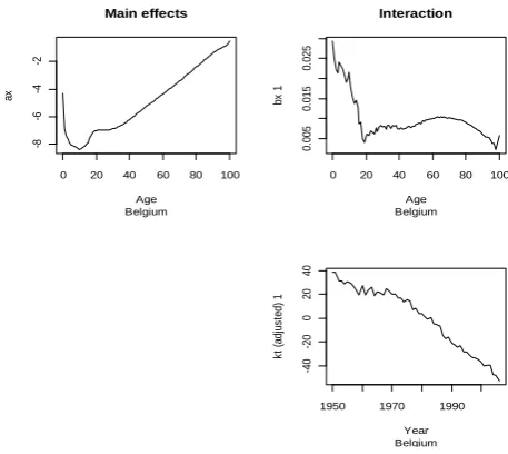
measures. In Figure 1, we show the estimates of the model parameters obtained by the fitting of the

LC model for the five considered countries:

0 20 40 60 80 100

-8

-6

-4

-2

Main effects

UK Age

ax

0 20 40 60 80 100

0

.0

0

5

0

.0

1

5

UK Age

b

x

1

Interaction

UK Year

k

t

(a

d

ju

s

te

d

)

1

1950 1970 1990

-4

0

-2

0

0

20

40

0 20 40 60 80 100

-8

-6

-4

-2

Main effects

France Age

ax

0 20 40 60 80 100

0

.0

0

5

0

.0

1

5

0

.0

2

5

France Age

b

x

1

Interaction

France Year

k

t

(a

d

ju

s

te

d

)

1

1950 1970 1990

-6

0

-2

0

0

20

40

0 20 40 60 80 100

-8

-6

-4

-2

Main effects

Italy Age

ax

0 20 40 60 80 100

0

.0

0

5

0

.0

1

5

0

.0

2

5

Italy Age

b

x

1

Interaction

Italy Year

k

t

(a

d

ju

s

te

d

)

1

1950 1970 1990

-6

0

-2

0

20

0 20 40 60 80 100

-8

-6

-4

-2

Main effects

Spain Age

ax

0 20 40 60 80 100

0

.0

0

0

0

.0

1

5

0

.0

3

0

Spain Age

b

x

1

Interaction

Spain Year

k

t

(a

d

ju

s

te

d

)

1

1950 1970 1990

-6

0

-2

0

20

0 20 40 60 80 100

-8

-6

-4

-2

Main effects

Belgium Age

ax

0 20 40 60 80 100

0.

00

5

0.

01

5

0.

02

5

Belgium Age

bx

1

Interaction

Belgium Year

kt

(

ad

ju

st

ed

)

1

1950 1970 1990

-4

0

-2

0

0

20

40

Figure 1- ax, bx, kt adjusted, basic Lee Carter model – UK, France, Italy, Spain, Belgium, total population, age: from 0 to 110

Observing Figure 1, we note that the fitting of the parameter _x is quite similar for each country:

the average of the mortality rate calculated during the years for a given age does not show significant differences across countries. Moreover, we can notice on the basis of the fitting of the

parameter kt that all countries have experienced a decreasing mortality trend during the years, with

a small difference in the rate of reduction. For example, Italy shows a lower rate of mortality reduction until 1980 and afterwards its acceleration. Instead, greater differences are recognized in

the fitting of the parameter x, which represents how different ages react to the reduction in

mortality. It presents a greater variability between age 30 to 100 in the Spanish dataset and between age 0 to 20 in the Belgian dataset. This feature has impact on the percentage of the variation explained in fitting the model, that is respectively: 93.3% for UK, 93.7% for France, 94.7% for Italy, 92% for Spain and 88.6% for Belgium. Furthermore, for each country, we compute the error measures on mortality rates. In Table 1 are shown the error measure findings with various indexes of the fitting accuracy averaged across years (ME=mean error, MSE=mean squared error, MPE=mean percentage error and MAPE=mean absolute percentage error), and also whose integrated across ages (IE=integrated error, ISE=integrated squared error, IPE=integrated percentage error and IAPE=integrated absolute percentage error):

Averages across ages:

ME MSE MPE MAPE

UK -0.00001 0.00005 0.00527 0.05513

France 0.00005 0.00009 0.00741 0.05645

Italy 0.00008 0.00008 0.0111 0 0.07269

Spain -0.00010 0.00008 0.00994 0.09113

Belgium -0.00021 0.00038 0.00926 0.07280

Averages across years:

IE ISE IPE IAPE

UK -0.00034 0.00395 0.52529 5.41629

France 0.00601 0.00612 0.73746 5.52106

Italy 0.00833 0.00573 1.11463 7.16246

Spain -0.00944 0.00693 0.99988 8.97029

Belgium -0.01393 0.02343 0.90969 6.92477

5.2 Measuring Dependence Structures

In the second stage of the numerical application, we measure either the dependence within each

single population, either the dependence between different populations: respectively the

intra-dependence and the inter-dependence. In that respect by focusing on the intra-dependence, we

include graphical analysis on autocorrelation functions by age and time, formal statistical tests as the Ljung-Box test based on the autocorrelation plot and Pearson test of independence. Regarding

the inter-dependence, we investigate the long-run relationships between countries by VAR scheme.

Thus, as regard the intra-dependence, broadly speaking the empirical evidences confirm a

dependence structure for each country. Going more deep into details, we make use of the correlogram, a graphical tool to examine the strength of association between observations, in order to investigate the correlation in the residuals. In the Appendix, we show the correlogram for each country, constructed by considering the correlation between ages for each year of the dataset. Throughout the correlograms, we can notice the persistence of correlation for UK, Italy and Spain almost always during the years. In other words, calculating the correlation means there is a dependence structure between ages in the same year and this appears for each year separately

considered: given t, we observe correlation between the residuals of age x0,1, 2, ,p, where p

is the maximum lag considered. In a different way, for France and Belgium the dependence outcome seems to be not so quite marked.

Furthermore in the Appendix, we show the correlogram by considering the correlation between years for each age. In this case, for each age, we are dealing with a time series generated from a stochastic process and verify the autocorrelation during the time. In other word, by considering the

dependence for a fixed t, we verify a temporal dependence for each age during the years. It is

possible to note that Italy and Spain prove a strong dependence structure for almost all ages, in particular for younger ones, which tends to decrease for adult ages. The case of UK shows a low correlation for younger ages, different from Italy, while it increases from 24-25 years up to 70

years. Also for France the correlation is stronger for the central ages instead of the extremes (lower

or higher ages). Belgium seems to have less marked dependence structure.

The graphical analysis is supported also by the results of Liung-Box test, implemented for each age and for each country separately.

On the basis of the calculations performed for each countries we can conclude that most for any age and for each country, the null hypothesis of independence is rejected. If we look at the p-value, i.e. the probability to make an error if we reject the null hypothesis when this is true, the value is very small for every age. In other words, we can confirm the randomness of the residuals, already observed in the graphical analysis.

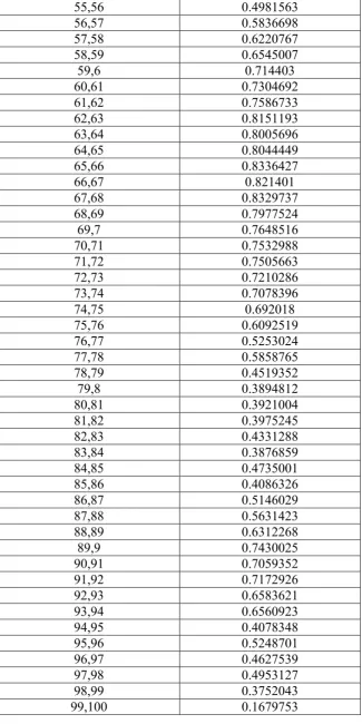
Finally, we compute the Pearson’s correlation coefficient, which assumes normality in the residuals distribution, and it confirms a strong positive dependence for almost all countries, except Spain and Belgium which present few negative values for some ages. For instance, table 2 illustrates the case of Italy.

Pearson’s correlation coefficient

x=age Value

0,1 0.9249975

1,2 0.9593225

2,3 0.9616913

3,4 0.91959

5,6 0.8806236

6,7 0.7955352

7,8 0.7433184

8,9 0.6569047

9,10 0.6516526

11,12 0.6837091

12,13 0.6134128

13,14 0.7446103

14,15 0.6364435

15,16 0.5834051

16,17 0.161985

17,18 0.6298621

18,19 0.3826222

19,20 0.6161803

20,21 0.537574

21,22 0.7511346

22,23 0.6995258

23,24 0.7612173

24,25 0.82023

25,26 0.8967373

26,27 0.9136936

27,28 0.8928995

28,29 0.8973545

29,3 0.9353529

30,31 0.9362392

31,32 0.9336044

32,33 0.940451

33,34 0.9311992

34,35 0.9343669

35,36 0.9261032

36,37 0.8973486

37,38 0.880285

38,39 0.8352225

39,40 0.8086334

40,41 0.853257

41,42 0.6992298

42,43 0.6305726

43,44 0.6976953

44,45 0.6622836

45,46 0.5847089

46,47 0.5756761

47,48 0.564031

48,49 0.4790489

49,50 0.5914199

50,51 0.4351083

51,52 0.5762156

52,53 0.608357

53,54 0.6347328

55,56 0.4981563

56,57 0.5836698

57,58 0.6220767

58,59 0.6545007

59,6 0.714403

60,61 0.7304692

61,62 0.7586733

62,63 0.8151193

63,64 0.8005696

64,65 0.8044449

65,66 0.8336427

66,67 0.821401

67,68 0.8329737

68,69 0.7977524

69,7 0.7648516

70,71 0.7532988

71,72 0.7505663

72,73 0.7210286

73,74 0.7078396

74,75 0.692018

75,76 0.6092519

76,77 0.5253024

77,78 0.5858765

78,79 0.4519352

79,8 0.3894812

80,81 0.3921004

81,82 0.3975245

82,83 0.4331288

83,84 0.3876859

84,85 0.4735001

85,86 0.4086326

86,87 0.5146029

87,88 0.5631423

88,89 0.6312268

89,9 0.7430025

90,91 0.7059352

91,92 0.7172926

92,93 0.6583621

93,94 0.6560923

94,95 0.4078348

95,96 0.5248701

96,97 0.4627539

97,98 0.4953127

98,99 0.3752043

99,100 0.1679753

Table 3 - Pearson Coefficient, Italy

At this last stage, after having assessed the dependence structures, we apply the Multiple Lee Carter Panel Sieve algorithm, described in Section 4, considering the datasets of UK, France, Italy, Spain and Belgium. Figure 2 plots estimates of k_t simultaneously, for the total population of the five

countries considered. As shown, k_t declines roughly linearly from 1950 to 2006, especially for

France and Italy.

Figure 2-, kt trends– UK, France, Italy, Spain, Belgium, Total population, years: from 1950 to 2006

We fit the VAR on the k_t of each country and calculate the residuals. Figures 3-7 display, for each

country, a diagram of fit, a residual plot, the auto-correlation and partial auto-correlation function of the residuals. For each country, we can observe that the autocorrelation and partial autocorrelation functions are consistent with the hypothesis of stationary series.

-40

-20

0

20

Diagram of fit and residuals for bel

0 10 20 30 40 50

-1

0

1

2

0 2 4 6 8 10 12

-0.

2

0.6

Lag ACF Re sidua ls

2 4 6 8 10 12

-0.

3

0.1

Lag PACF Re sidua ls

Figure 4- Diagram of fit, residuals, ACF and PACF of residuals for Belgium

Figure 6- Diagram of fit, residuals, ACF and PACF of residuals for France

Figure 7- Diagram of fit, residuals, ACF and PACF of residuals for Italy

Finally, we simulate for each period the k_t medium, by implementing a bootstrap on the basis of

the algorithm indicated in Section 4. Then, we project them by using ARIMA models and calculate

confidence intervals. Figures 8 displays the mean of the simulated k_t and the projections with

Figure 8- mean kt for UK, Belgium, Spain, France and Italy

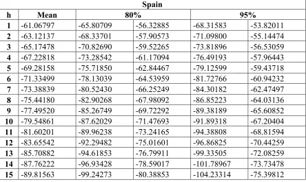
Table 3-7 illustrate the mean of projection of kt for h1, ,15 periods ahead, calculated running a

number of simulations equal to 1000. Moreover, the 80% and 95% confidence intervals values are shown in the same tables for each countries.

Table 3- Confidence Intervals for kt, 80% and 95%, UK

UK

h Mean 80% 95%

1 -50.87365 -55.18137 -46.56592 -57.46174 -44.28555

2 -55.19162 -59.84698 -50.53625 -62.31138 -48.07185

3 -55.13368 -60.82036 -49.44701 -63.83070 -46.43666

4 -57.65851 -63.82319 -51.49382 -67.08658 -48.23044

5 -58.65893 -65.47290 -51.84496 -69.08000 -48.23786

6 -60.55909 -67.85024 -53.26794 -71.70995 -49.40823

7 -61.92820 -69.73011 -54.12630 -73.86019 -49.99622

8 -63.61075 -71.85655 -55.36495 -76.22161 -50.99989

9 -65.10830 -73.79504 -56.42157 -78.39352 -51.82309

10 -66.71505 -75.81023 -57.61987 -80.62492 -52.80517

11 -68.25734 -77.74970 -58.76498 -82.77465 -53.74003

12 -69.83767 -79.70766 -59.96769 -84.93252 -54.74283

13 -71.39556 -81.63129 -61.15983 -87.04976 -55.74136

14 -72.96669 -83.55438 -62.37901 -89.15916 -56.77422

Table 4- Confidence Intervals for kt, 80% and 95%, Belgium

Table 5- Confidence Intervals for kt, 80% and 95%, Spain

Belgium

h Mean 80% 95%

1 -50.16977 -54.76127 -45.57827 -57.19186 -43.14768

2 -51.71650 -56.83237 -46.60064 -59.54054 -43.89247

3 -53.26324 -58.85450 -47.67197 -61.81434 -44.71213

4 -54.80997 -60.83927 -48.78067 -64.03098 -45.58895

5 -56.35670 -62.79430 -49.91911 -66.20215 -46.51125

6 -57.90343 -64.72493 -51.08194 -68.33601 -47.47086

7 -59.45017 -66.63508 -52.26525 -70.43854 -48.46179

8 -60.99690 -68.52772 -53.46608 -72.51429 -49.47951

9 -62.54363 -70.40514 -54.68212 -74.56678 -50.52049

10 -64.09037 -72.26921 -55.91152 -76.59883 -51.58190

11 -65.63710 -74.12142 -57.15277 -78.61275 -52.66145

12 -67.18383 -75.96301 -58.40466 -80.61042 -53.75724

13 -68.73056 -77.79501 -59.66612 -82.59343 -54.86770

14 -70.27730 -79.61830 -60.93630 -84.56313 -55.99147

15 -71.82403 -81.43363 -62.21443 -86.52065 -57.12741

Spain

h Mean 80% 95%

1 -61.06797 -65.80709 -56.32885 -68.31583 -53.82011

2 -63.12137 -68.33701 -57.90573 -71.09800 -55.14474

3 -65.17478 -70.82690 -59.52265 -73.81896 -56.53059

4 -67.22818 -73.28542 -61.17094 -76.49193 -57.96443

5 -69.28158 -75.71850 -62.84467 -79.12599 -59.43718

6 -71.33499 -78.13039 -64.53959 -81.72766 -60.94232

7 -73.38839 -80.52430 -66.25249 -84.30182 -62.47497

8 -75.44180 -82.90268 -67.98092 -86.85223 -64.03136

9 -77.49520 -85.26749 -69.72292 -89.38189 -65.60852

10 -79.54861 -87.62029 -71.47693 -91.89318 -67.20404

11 -81.60201 -89.96238 -73.24165 -94.38808 -68.81594

12 -83.65542 -92.29482 -75.01601 -96.86825 -70.44259

13 -85.70882 -94.61853 -76.79911 -99.33505 -72.08259

14 -87.76222 -96.93428 -78.59017 -101.78967 -73.73478

15 -89.81563 -99.24273 -80.38853 -104.23314 -75.39812

Table 6- Confidence Intervals for kt, 80% and 95%, France

Table 7- Confidence Intervals for kt, 80% and 95%, Italy

h Mean 80% 95%

1 -54.40954 -59.09458 -49.72451 -61.57469 -47.24440

2 -57.53012 -62.21537 -52.84486 -64.69560 -50.36463

3 -60.27504 -65.02405 -55.52603 -67.53802 -53.01205

4 -62.75654 -67.67673 -57.83634 -70.28133 -55.23175

5 -65.05331 -70.24118 -59.86544 -72.98747 -57.11915

6 -67.22054 -72.74407 -61.69700 -75.66805 -58.77302

7 -69.29692 -75.19643 -63.39741 -78.31944 -60.27440

8 -71.30960 -77.60455 -65.01465 -80.93690 -61.68231

9 -73.27761 -79.97363 -66.58159 -83.51829 -63.03693

10 -75.21429 -82.30852 -68.12006 -86.06397 -64.36461

11 -77.12900 -84.61372 -69.64429 -88.57589 -65.68212

12 -79.02831 -86.89325 -71.16336 -91.05670 -66.99991

13 -80.91681 -89.15061 -72.68301 -93.50932 -68.32430

14 -82.79774 -91.38874 -74.20673 -95.93655 -69.65893

15 -84.67335 -93.61013 -75.73658 -98.34097 -71.00573

Italy

h Mean 80% 95%

1 -73.52702 -79.08849 -67.96555 -82.03255 -65.02148

2 -75.76981 -81.99289 -69.54672 -85.28720 -66.25242

3 -78.01260 -84.83342 -71.19178 -88.44415 -67.58105

4 -80.25539 -87.62563 -72.88515 -91.52720 -68.98358

5 -82.49818 -90.37963 -74.61673 -94.55182 -70.44454

6 -84.74097 -93.10243 -76.37950 -97.52872 -71.95321

7 -86.98376 -95.79914 -78.16838 -100.46572 -73.50180

8 -89.22655 -98.47359 -79.97951 -103.36867 -75.08442

9 -91.46934 -101.12877 -81.80991 -106.24216 -76.69651

10 -93.71213 -103.76705 -83.65721 -109.08980 -78.33445

11 -95.95492 -106.39035 -85.51948 -111.91453 -79.99530

12 -98.19771 -109.00025 -87.39516 -114.71878 -81.67663

13 -100.44050 -111.59809 -89.28290 -117.50456 -83.37643

14 -102.68329 -114.18497 -91.18160 -120.27359 -85.09298

6 Concluding Remarks

Several models have been developed for representing future mortality trends. In particular, the extrapolative methods allow for obtaining the most reliable approach in terms of forecast accuracy. Among the class of models under consideration, we base our work round the Lee-Carter one,

because its desirable features (Tuljapurkar et al. 2000). Therefore, in this paper we try to develop a

more accurate algorithm in terms of prediction intervals. To do this, an improved predictor should take into account not only the dependence across age and time (D’Amato et al. 2012b), but also the dependence structure across different populations characterized by similar feature, so that potentially affected by common factors.

We present an algorithm that preserve the parametric structure in Lee Carter setting, as well as improve the goodness of the predictor in its genetic construction, because it is in the context of the appropriate tools for bootstrap simulation of dependent data. Other interesting research questions are worth exploring. Whilst the presence of cross sectional dependence is considered in our framework, the standard LC model can be extended to accommodate for the presence of several common stochastic trends (as opposed to only one) and to include the presence of stationary common factors in the error term. The latter extension, in particular, could prove useful in order to take into account the presence of strong cross sectional dependence across units (i.e. across countries and age groups). This is a very important topic, since the bootstrap algorithm proposed here, per se, is a “one cross sectional unit at a time” algorithm, which ensures consistency only in presence of weak cross dependence. Trapani (2013) discusses some extensions of the bootstrap theory to the case of multiple, stationary and nonstationary common trends. The application of such theory to the context of the LC model is currently under investigation by the authors.

Next issues related to the topic will focus on the proof of accuracy of the proposed method.

References

Anderson, T. W., 1984, An Introduction to Multivariate Statistical Analysis, 2nd Edition, New

York: Wiley

Bai, J., 2004, Estimating cross-section common stochastic trends in nonstationary panel data,

Journal of Econometrics, 122, 137-183

Booth, H., Maindonald J., Smith, L., 2002, Age-time interactions in mortality projections: applying Lee-Carter to Australia. Working Papers in Demography n. 85

Bühlmann, P., 1997, Sieve bootstrap for time series, Bernoulli, 3, 123-148

Cairns, A.J.G., D. Blake, K. Dowd, G.D. Coughlan, M. Khalaf-Allah, 2011, Bayesian Stochastic

Mortality Modelling for Two Populations. ASTIN Bulletin, 41(1), 29–59.

D’Amato V., Haberman S., Russolillo M., 2012a, The Stratified Sampling Bootstrap: an algorithm for measuring the uncertainty in forecast mortality rates in the Poisson Lee-Carter setting.

Methodology and Computing in Applied Probability, 14(1), 135-148.

D’Amato V., Di Lorenzo E., Haberman S., Russolillo M., Sibillo M., 2011, The Poisson

log-bilinear Lee Carter model: Applications of efficient bootstrap methods to annuity analyses. North

http://www.soa.org/library/journals/north-american-actuarial-journal/2011/no-2/naaj-2011-vol15-no2.aspx

D’Amato V., Haberman S., Piscopo G., Russolillo M., 2012b, Modelling dependent data for

longevity projections. Insurance Mathematics and Economics 51, 694-701, DOI information:

10.1016/j.insmatheco.2012.09.008

Fiig Jarner, S., E. Masotty Kryger, 2009, Modelling adult mortality in small populations: the Saint

model. Pensions Institute DiscussionPaper PI-0902.

Gaille S., Sherris M., 2011, Modelling Mortality with Common Stochastic Long-Run Trends. The

Geneva Papers on Risk and Insurance - Issues and Practice, 36(4), 595-621.

Hainut D., 2012, Multidimensional Lee–Carter model with switching mortality processes.

Insurance Mathematics and Economics, 50(2), 236-246.

Lazar, D., Denuit, M., 2009, A multivariate time series approach to projected life tables. Applied

Stochastic Models in Business and Industry,25, 806–823.

Lee, R.D., L. R. Carter, 1992, Modelling and Forecasting U.S. Mortality. Journal of the American

Statistical Association, 87, 659-671.

Li, N., R. Lee, 2005, Coherent mortality forecasts for a group of populations: An extension of the

Lee-Carter method. Demography, 42(3), 575–594.

Li, J. S. H., Hardy, M. R., 2011, Measuring Basis Risk Involved in Longevity Hedges. North

American Actuarial Journal, 15(2), 177–200.

Olivieri A., 2011, Forecasting mortality by mixing mortality experiences, Demography and Longevity Workshop, CEPAR Sydney

Russolillo, M., Giordano, G., Haberman, S., 2011, Extending the Lee-Carter model: a three-way

decomposition. Scandinavian Actuarial Journal, 2, 96-117.

Stevens, R., 2011, A time-dependent age-factor extension to the Lee- Carter model, Longevity 7, Frankfurt

Trapani, L., 2012, On bootstrapping panel factor series - Extended version. Available at SSRN:

http://ssrn.com/abstract=2062183

Trapani, L., 2013, On bootstrapping panel factor series. Journal of Econometrics, 172, 127-141.

Tuljapurkar, S, Li, N and Boe, C, 2000, A universal pattern of mortality decline in the G7 countries.

Nature, 405, 789-792.

United Nations, 1998, World Populations Prospects: The 1996 Revision. New York: Population Division, United Nations.

White, K. M., 2002, Longevity Advances in High-income Countries, 1955–96. Population and

Wilson, C, 2001, On the Scale of Global Demographic Convergence 1950–2000. Population and Development Review, 24, 593–600.

Appendix

UK, correlograms between ages for each year, where t=1 corresponds to 1950 up to t=56 which represents 2006 calendar year.

0 5 10 20

-0 .2 0. 2 0. 6 1. 0 Lag AC F t=1

0 5 10 20

-0 .2 0. 4 1. 0 Lag AC F t=2

0 5 10 20

-0 .2 0. 2 0. 6 1. 0 Lag AC F t=3

0 5 10 20

-0 .2 0. 2 0. 6 1. 0 Lag AC F t=4

0 5 10 20

-0 .2 0. 4 0. 8 Lag AC F t=5

0 5 10 20

-0 .2 0. 2 0. 6 1. 0 Lag AC F t=6

0 5 10 20

-0 .2 0. 4 0. 8 Lag AC F t=7

0 5 10 20

-0 .2 0. 2 0. 6 1. 0 Lag AC F t=8

0 5 10 20

-0 .2 0. 2 0. 6 1. 0 Lag AC F t=9

0 5 10 20

-0 .2 0. 2 0. 6 1. 0 Lag AC F t=10

0 5 10 20

-0 .2 0. 2 0. 6 1. 0 Lag AC F t=11

0 510 20

-0 .2 0. 2 0. 6 1. 0 Lag AC F t=12

0 5 10 20

-0 .2 0. 2 0. 6 1. 0 Lag AC F t=13

0 5 10 20

-0 .2 0. 2 0. 6 1. 0 Lag AC F t=14

0 510 20

-0 .2 0. 2 0. 6 1. 0 Lag AC F t=15

0 5 10 20

-0 .2 0. 4 0. 8 Lag AC F t=16

0 5 10 20

-0 .2 0. 4 0. 8 Lag AC F t=17

0 510 20

-0 .2 0. 4 0. 8 Lag AC F t=18

0 510 20

-0 .2 0. 4 1. 0 Lag AC F t=19

0 5 10 20

-0 .2 0. 2 0. 6 1. 0 Lag AC F t=20

0 5 10 20

-0 .2 0. 4 0. 8 Lag AC F t=21

0 510 20

-0 .5 0. 0 0. 5 1. 0 Lag AC F t=22

0 5 10 20

-0 .2 0. 4 0. 8 Lag AC F t=23

0 5 10 20

-0 .2 0. 4 0. 8 Lag AC F t=24

0 510 20

-0 .2 0. 2 0. 6 1. 0 Lag AC F t=25

0 5 10 20

-0 .2 0. 4 0. 8 Lag AC F t=26

0 5 10 20

-0 .2 0. 2 0. 6 1. 0 Lag AC F t=27

0 5 10 20

-0 .2 0. 2 0. 6 1. 0 Lag AC F t=28

0 510 20

-0 .2 0. 4 0. 8 Lag AC F t=29

0 510 20

-0 .2 0. 2 0. 6 1. 0 Lag AC F t=30

0 5 10 20

-0 .2 0. 2 0. 6 1. 0 Lag AC F t=31

0 510 20

-0 .2 0. 2 0. 6 1. 0 Lag AC F t=32

0 510 20

-0 .2 0. 2 0. 6 1. 0 Lag AC F t=33

0 5 10 20

-0 .2 0. 2 0. 6 1. 0 Lag AC F t=34

0 510 20

-0 .2 0. 4 0. 8 Lag AC F t=35

0 510 20

-0 .2 0. 2 0. 6 1. 0 Lag AC F t=36

0 510 20

-0 .2 0. 2 0. 6 1. 0 Lag A C F t=37

0 5 10 20

-0 .2 0. 2 0. 6 1. 0 Lag A C F t=38

0 510 20

-0 .2 0. 2 0. 6 1. 0 Lag A C F t=39

0 510 20

-0 .2 0. 2 0. 6 1. 0 Lag A C F t=40

0 5 10 20

-0 .2 0. 4 1. 0 Lag A C F t=41

0 510 20

-0 .2 0. 4 0. 8 Lag A C F t=42

0 510 20

-0 .2 0. 4 1. 0 Lag A C F t=43

0 5 10 20

-0 .2 0. 2 0. 6 1. 0 Lag A C F t=44

0 510 20

France, correlograms between ages for each year, where t=1 corresponds to 1950 up to t=56 which represents 2006 calendar year.

0 5 10 20

-0 .2 0. 2 0. 6 1. 0 Lag A C F t=1

0 5 10 20

-0 .2 0. 2 0. 6 1. 0 Lag A C F t=2

0 5 10 20

-0 .2 0. 2 0. 6 1. 0 Lag A C F t=3

0 5 10 20

-0 .2 0. 2 0. 6 1. 0 Lag A C F t=4

0 5 10 20

-0 .2 0. 4 0. 8 Lag A C F t=5

0 5 10 20

-0 .2 0. 4 0. 8 Lag A C F t=6

0 5 10 20

-0 .2 0. 2 0. 6 1. 0 Lag A C F t=7

0 5 10 20

-0 .2 0. 4 0. 8 Lag A C F t=8

0 5 10 20

-0 .2 0. 4 0. 8 Lag A C F t=9

0 5 10 20

-0 .2 0 .4 0 .8 Lag A C F t=10

0 5 10 20

-0 .2 0 .2 0 .6 1 .0 Lag A C F t=11

0 5 10 20

-0 .2 0 .4 0 .8 Lag A C F t=12

0 5 10 20

-0 .2 0 .2 0 .6 1 .0 Lag A C F t=13

0 5 10 20

-0 .2 0 .2 0 .6 1 .0 Lag A C F t=14

0 5 10 20

-0 .2 0 .2 0 .6 1 .0 Lag A C F t=15

0 5 10 20

-0 .2 0 .2 0 .6 1 .0 Lag A C F t=16

0 5 10 20

-0 .2 0 .2 0 .6 1 .0 Lag A C F t=17

0 5 10 20

-0 .2 0 .2 0 .6 1 .0 Lag A C F t=18

0 5 10 20

-0 .2 0 .4 1 .0 Lag A C F t=19

0 5 10 20

-0 .2 0 .4 1 .0 Lag A C F t=20

0 5 10 20

-0 .4 0 .2 0 .8 Lag A C F t=21

0 5 10 20

-0 .4 0 .2 0 .8 Lag A C F t=22

0 5 10 20

-0 .2 0 .4 0 .8 Lag A C F t=23

0 5 10 20

-0 .4 0 .2 0 .8 Lag A C F t=24

0 5 10 20

-0 .4 0 .2 0 .8 Lag A C F t=25

0 5 10 20

-0 .5 0 .0 0 .5 1 .0 Lag A C F t=26

0 5 10 20

-0 .5 0 .5 1 .0 Lag A C F t=27

0 5 10 20

-0 .4 0. 2 0. 8 Lag A C F t=28

0 5 10 20

0. 0 0. 5 1. 0 Lag A C F t=29

0 5 10 20

-0 .4 0. 2 0. 8 Lag A C F t=30

0 5 10 20

-0 .2 0. 4 1. 0 Lag A C F t=31

0 5 10 20

-0 .4 0. 2 0. 8 Lag A C F t=32

0 5 10 20

-0 .2 0. 4 1. 0 Lag A C F t=33

0 5 10 20

-0 .2 0. 4 1. 0 Lag A C F t=34

0 5 10 20

-0 .2 0. 4 0. 8 Lag A C F t=35

0 5 10 20

0 5 10 20 -0 .2 0 .4 0 .8 Lag A C F t=37

0 5 10 20

-0 .2 0 .2 0 .6 1 .0 Lag A C F t=38

0 5 10 20

-0 .2 0 .2 0 .6 1 .0 Lag A C F t=39

0 5 10 20

-0 .2 0 .2 0 .6 1 .0 Lag A C F t=40

0 5 10 20

-0 .2 0 .2 0 .6 1 .0 Lag A C F t=41

0 5 10 20

-0 .2 0 .2 0 .6 1 .0 Lag A C F t=42

0 5 10 20

-0 .2 0 .2 0 .6 1 .0 Lag A C F t=43

0 5 10 20

-0 .2 0 .2 0 .6 1 .0 Lag A C F t=44

0 5 10 20

-0 .2 0 .2 0 .6 1 .0 Lag A C F t=45 0 15 -0 .2 1. 0 Lag A C F t=46 0 15 -0 .2 1. 0 Lag A C F t=47 0 15 -0 .2 1. 0 Lag A C F t=48 0 15 -0 .2 1. 0 Lag A C F t=49 0 15 -0 .2 1. 0 Lag A C F t=50 0 15 -0 .2 1. 0 Lag A C F t=51 0 15 -0 .2 1. 0 Lag A C F t=52 0 15 -0 .2 1. 0 Lag A C F t=53 0 15 -0 .2 1. 0 Lag A C F t=54 0 15 -0 .2 1. 0 Lag A C F t=55 0 15 -0 .2 1. 0 Lag A C F t=56

Italy, correlograms between ages for each year, where t=1 corresponds to 1950 up to t=56 which represents 2006 calendar year.

0 5 10 20

-0 .2 0. 2 0. 6 1. 0 Lag A C F t=1

0 5 10 20

-0 .2 0. 2 0. 6 1. 0 Lag A C F t=2

0 5 10 20

-0 .2 0. 2 0. 6 1. 0 Lag A C F t=3

0 5 10 20

-0 .2 0. 2 0. 6 1. 0 Lag A C F t=4

0 5 10 20

-0 .2 0. 2 0. 6 1. 0 Lag A C F t=5

0 5 10 20

-0 .2 0. 2 0. 6 1. 0 Lag A C F t=6

0 5 10 20

-0 .2 0. 2 0. 6 1. 0 Lag A C F t=7

0 5 10 20

-0 .2 0. 2 0. 6 1. 0 Lag A C F t=8

0 5 10 20

-0 .2 0. 2 0. 6 1. 0 Lag A C F t=9

0 5 10 20

-0 .2 0 .2 0 .6 1 .0 Lag A C F t=10

0 5 10 20

-0 .2 0 .4 0 .8 Lag A C F t=11

0 510 20

-0 .2 0 .2 0 .6 1 .0 Lag A C F t=12

0 5 10 20

-0 .2 0 .4 0 .8 Lag A C F t=13

0 5 10 20

-0 .2 0 .4 0 .8 Lag A C F t=14

0 510 20

-0 .2 0 .2 0 .6 1 .0 Lag A C F t=15

0 5 10 20

-0 .2 0 .2 0 .6 1 .0 Lag A C F t=16

0 5 10 20

-0 .2 0 .2 0 .6 1 .0 Lag A C F t=17

0 510 20

-0 .2 0 .2 0 .6 1 .0 Lag A C F t=18

0 5 10 20

-0 .2 0. 2 0. 6 1. 0 Lag AC F t=19

0 5 10 20

-0 .2 0. 2 0. 6 1. 0 Lag AC F t=20

0 5 10 20

-0 .2 0. 2 0. 6 1. 0 Lag AC F t=21

0 5 10 20

-0 .2 0. 2 0. 6 1. 0 Lag AC F t=22

0 5 10 20

-0 .2 0. 4 0. 8 Lag AC F t=23

0 5 10 20

-0 .2 0. 2 0. 6 1. 0 Lag AC F t=24

0 5 10 20

-0 .2 0. 2 0. 6 1. 0 Lag AC F t=25

0 5 10 20

-0 .2 0. 2 0. 6 1. 0 Lag AC F t=26

0 5 10 20

-0 .2 0. 2 0. 6 1. 0 Lag AC F t=27

0 510 20

-0 .2 0 .2 0 .6 1 .0 Lag A C F t=28

0 510 20

-0 .2 0 .2 0 .6 1 .0 Lag A C F t=29

0 510 20

-0 .2 0 .2 0 .6 1 .0 Lag A C F t=30

0 510 20

-0 .2 0 .2 0 .6 1 .0 Lag A C F t=31

0 510 20

-0 .2 0 .2 0 .6 1 .0 Lag A C F t=32

0 510 20

-0 .2 0 .2 0 .6 1 .0 Lag A C F t=33

0 510 20

-0 .2 0 .2 0 .6 1 .0 Lag A C F t=34

0 510 20

-0 .2 0 .2 0 .6 1 .0 Lag A C F t=35

0 510 20

0 5 10 20 -0 .2 0. 2 0. 6 1. 0 Lag A C F t=37

0 5 10 20

-0 .2 0. 2 0. 6 1. 0 Lag A C F t=38

0 5 10 20

-0 .2 0. 2 0. 6 1. 0 Lag A C F t=39

0 5 10 20

-0 .4 0. 2 0. 8 Lag A C F t=40

0 5 10 20

-0 .4 0. 2 0. 8 Lag A C F t=41

0 5 10 20

-0 .4 0. 2 0. 8 Lag A C F t=42

0 5 10 20

-0 .2 0. 2 0. 6 1. 0 Lag A C F t=43

0 5 10 20

-0 .2 0. 2 0. 6 1. 0 Lag A C F t=44

0 5 10 20

-0 .2 0. 2 0. 6 1. 0 Lag A C F t=45 0 15 -0 .2 1. 0 Lag A C F t=46 0 15 -0 .2 1. 0 Lag A C F t=47 0 15 -0 .2 1. 0 Lag A C F t=48 0 15 -0 .2 1. 0 Lag A C F t=49 0 15 -0 .2 1. 0 Lag A C F t=50 0 15 -0 .2 1. 0 Lag A C F t=51 0 15 -0 .2 1. 0 Lag A C F t=52 0 15 -0 .2 1. 0 Lag A C F t=53 0 15 -0 .2 1. 0 Lag A C F t=54 0 15 -0 .2 1. 0 Lag A C F t=55 0 15 -0 .2 1. 0 Lag A C F t=56

Spain, correlograms between ages for each year, where t=1 corresponds to 1950 up to t=56 which represents 2006 calendar year.

0 5 10 20

-0 .2 0. 2 0. 6 1. 0 Lag A C F t=1

0 5 10 20

-0 .2 0. 2 0. 6 1. 0 Lag A C F t=2

0 5 10 20

-0 .2 0. 2 0. 6 1. 0 Lag A C F t=3

0 5 10 20

-0 .2 0. 2 0. 6 1. 0 Lag A C F t=4

0 5 10 20

-0 .2 0. 2 0. 6 1. 0 Lag A C F t=5

0 5 10 20

-0 .2 0. 2 0. 6 1. 0 Lag A C F t=6

0 5 10 20

-0 .2 0. 2 0. 6 1. 0 Lag A C F t=7

0 5 10 20

-0 .2 0. 2 0. 6 1. 0 Lag A C F t=8

0 5 10 20

-0 .2 0. 4 0. 8 Lag A C F t=9

0 5 10 20

-0 .2 0. 4 0. 8 Lag A C F t=10

0 5 10 20

-0 .2 0. 2 0. 6 1. 0 Lag A C F t=11

0 5 10 20

-0 .2 0. 2 0. 6 1. 0 Lag A C F t=12

0 5 10 20

-0 .2 0. 2 0. 6 1. 0 Lag A C F t=13

0 5 10 20

-0 .2 0. 2 0. 6 1. 0 Lag A C F t=14

0 5 10 20

-0 .2 0. 2 0. 6 1. 0 Lag A C F t=15

0 5 10 20

-0 .2 0. 2 0. 6 1. 0 Lag A C F t=16

0 5 10 20

-0 .2 0. 2 0. 6 1. 0 Lag A C F t=17

0 5 10 20

-0 .2 0. 2 0. 6 1. 0 Lag A C F t=18

0 510 20

-0 .2 0. 2 0. 6 1. 0 Lag AC F t=19

0 5 10 20

-0 .2 0. 2 0. 6 1. 0 Lag AC F t=20

0 510 20

-0 .2 0. 2 0. 6 1. 0 Lag AC F t=21

0 510 20

-0 .2 0. 2 0. 6 1. 0 Lag AC F t=22

0 5 10 20

-0 .2 0. 2 0. 6 1. 0 Lag AC F t=23

0 510 20

-0 .2 0. 2 0. 6 1. 0 Lag AC F t=24

0 510 20

-0 .2 0. 2 0. 6 1. 0 Lag AC F t=25

0 5 10 20

-0 .2 0. 2 0. 6 1. 0 Lag AC F t=26

0 510 20

-0 .2 0. 2 0. 6 1. 0 Lag AC F t=27

0 5 10 20

-0 .2 0. 2 0. 6 1. 0 Lag AC F t=28

0 5 10 20

-0 .2 0. 2 0. 6 1. 0 Lag AC F t=29

0 5 10 20

-0 .2 0. 4 0. 8 Lag AC F t=30

0 5 10 20

-0 .2 0. 2 0. 6 1. 0 Lag AC F t=31

0 5 10 20

-0 .2 0. 2 0. 6 1. 0 Lag AC F t=32

0 5 10 20

-0 .2 0. 4 0. 8 Lag AC F t=33

0 5 10 20

-0 .2 0. 2 0. 6 1. 0 Lag AC F t=34

0 5 10 20

-0 .2 0. 4 0. 8 Lag AC F t=35

0 5 10 20

0 510 20 -0 .2 0 .4 0 .8 Lag A C F t=37

0 5 10 20

-0 .2 0 .4 0 .8 Lag A C F t=38

0 510 20

-0 .2 0 .4 0 .8 Lag A C F t=39

0 510 20

-0 .2 0 .2 0 .6 1 .0 Lag A C F t=40

0 5 10 20

-0 .2 0 .2 0 .6 1 .0 Lag A C F t=41

0 510 20

-0 .2 0 .2 0 .6 1 .0 Lag A C F t=42

0 510 20

-0 .2 0 .2 0 .6 1 .0 Lag A C F t=43

0 5 10 20

-0 .2 0 .2 0 .6 1 .0 Lag A C F t=44

0 510 20

-0 .2 0 .2 0 .6 1 .0 Lag A C F t=45 0 15 -0 .2 1 .0 Lag A C F t=46 0 15 -0 .2 1 .0 Lag A C F t=47 0 15 -0 .2 1 .0 Lag A C F t=48 0 15 -0 .2 1 .0 Lag A C F t=49 0 15 -0 .2 1 .0 Lag A C F t=50 0 15 -0 .2 1 .0 Lag A C F t=51 0 15 -0 .2 1 .0 Lag A C F t=52 0 15 -0 .2 1 .0 Lag A C F t=53 0 15 -0 .2 1 .0 Lag A C F t=54 0 15 -0 .2 1 .0 Lag A C F t=55 0 15 -0 .2 1 .0 Lag A C F t=56

Belgium, correlograms between ages for each year, where t=1 corresponds to 1950 up to t=56 which represents 2006 calendar year.

0 5 10 20

-0 .2 0. 2 0. 6 1. 0 Lag AC F t=1

0 5 10 20

-0 .2 0. 2 0. 6 1. 0 Lag AC F t=2

0 5 10 20

-0 .2 0. 2 0. 6 1. 0 Lag AC F t=3

0 5 10 20

-0 .2 0. 4 0. 8 Lag AC F t=4

0 5 10 20

-0 .4 0. 2 0. 8 Lag AC F t=5

0 5 10 20

-0 .2 0. 4 1. 0 Lag AC F t=6

0 5 10 20

-0 .2 0. 4 0. 8 Lag AC F t=7

0 5 10 20

-0 .2 0. 2 0. 6 1. 0 Lag AC F t=8

0 5 10 20

-0 .2 0. 2 0. 6 1. 0 Lag AC F t=9

0 510 20

-0 .2 0. 2 0. 6 1. 0 Lag A C F t=10

0 510 20

-0 .2 0. 2 0. 6 1. 0 Lag A C F t=11

0 510 20

-0 .2 0. 2 0. 6 1. 0 Lag A C F t=12

0 510 20

-0 .2 0. 2 0. 6 1. 0 Lag A C F t=13

0 510 20

-0 .2 0. 2 0. 6 1. 0 Lag A C F t=14

0 510 20

-0 .2 0. 2 0. 6 1. 0 Lag A C F t=15

0 510 20

-0 .2 0. 2 0. 6 1. 0 Lag A C F t=16

0 510 20

-0 .2 0. 2 0. 6 1. 0 Lag A C F t=17

0 510 20

-0 .2 0. 2 0. 6 1. 0 Lag A C F t=18

0 5 10 20

-0 .2 0. 2 0. 6 1. 0 Lag AC F t=19

0 5 10 20

-0 .2 0. 2 0. 6 1. 0 Lag AC F t=20

0 5 10 20

-0 .2 0. 2 0. 6 1. 0 Lag AC F t=21

0 5 10 20

-0 .2 0. 4 0. 8 Lag AC F t=22

0 5 10 20

-0 .2 0. 4 0. 8 Lag AC F t=23

0 5 10 20

-0 .2 0. 2 0. 6 1. 0 Lag AC F t=24

0 5 10 20

-0 .2 0. 4 0. 8 Lag AC F t=25

0 5 10 20

-0 .2 0. 2 0. 6 1. 0 Lag AC F t=26

0 5 10 20

-0 .2 0. 2 0. 6 1. 0 Lag AC F t=27

0 5 10 20

-0 .2 0. 4 0. 8 Lag A C F t=28

0 5 10 20

-0 .2 0. 4 1. 0 Lag A C F t=29

0 5 10 20

-0 .2 0. 2 0. 6 1. 0 Lag A C F t=30

0 5 10 20

-0 .2 0. 2 0. 6 1. 0 Lag A C F t=31

0 5 10 20

-0 .2 0. 2 0. 6 1. 0 Lag A C F t=32

0 5 10 20

-0 .2 0. 4 0. 8 Lag A C F t=33

0 5 10 20

-0 .2 0. 2 0. 6 1. 0 Lag A C F t=34

0 5 10 20

-0 .2 0. 2 0. 6 1. 0 Lag A C F t=35

0 5 10 20

0 510 20 -0 .2 0. 4 0. 8 Lag AC F t=37

0 5 10 20

-0 .2 0. 2 0. 6 1. 0 Lag AC F t=38

0 510 20

-0 .2 0. 2 0. 6 1. 0 Lag AC F t=39

0 510 20

-0 .2 0. 2 0. 6 1. 0 Lag AC F t=40

0 5 10 20

-0 .2 0. 2 0. 6 1. 0 Lag AC F t=41

0 510 20

-0 .2 0. 2 0. 6 1. 0 Lag AC F t=42

0 510 20

-0 .2 0. 2 0. 6 1. 0 Lag AC F t=43

0 5 10 20

-0 .2 0. 4 0. 8 Lag AC F t=44

0 510 20

-0 .2 0. 2 0. 6 1. 0 Lag AC F t=45 0 15 -0 .2 1. 0 Lag AC F t=46 0 15 -0 .2 1. 0 Lag AC F t=47 0 15 -0 .2 1. 0 Lag AC F t=48 0 15 -0 .2 1. 0 Lag AC F t=49 0 15 -0 .2 1. 0 Lag AC F t=50 0 15 -0 .2 1. 0 Lag AC F t=51 0 15 -0 .2 1. 0 Lag AC F t=52 0 15 -0 .2 1. 0 Lag AC F t=53 0 15 -0 .2 1. 0 Lag AC F t=54 0 15 -0 .2 1. 0 Lag AC F t=55 0 15 -0 .2 1. 0 Lag AC F t=56

UK, correlograms between calendar years for each age.

0 5 10 15

-0 .2 0. 4 0. 8 Lag A C F x=1

0 5 10 15

-0 .2 0. 4 0. 8 Lag A C F x=2

0 5 10 15

-0 .2 0. 4 0. 8 Lag A C F x=3

0 5 10 15

-0 .2 0. 4 0. 8 Lag A C F x=4

0 5 10 15

-0 .2 0. 4 0. 8 Lag A C F x=5

0 5 10 15

-0 .2 0. 4 0. 8 Lag A C F x=6

0 5 10 15

-0 .2 0. 4 0. 8 Lag A C F x=7

0 5 10 15

-0 .2 0. 4 0. 8 Lag A C F x=8

0 5 1015

-0 .2 0. 4 0. 8 Lag A C F x=9

0 5 10 15

-0 .2 0. 4 1. 0 Lag A C F x=10

0 5 1015

-0 .2 0. 4 0. 8 Lag A C F x=11

0 5 1015

-0 .2 0. 4 0. 8 Lag A C F x=12

0 5 10 15

-0 .2 0. 4 0. 8 Lag A C F x=13

0 5 1015

-0 .2 0. 4 0. 8 Lag A C F x=14

0 5 1015

-0 .2 0. 4 0. 8 Lag A C F x=15

0 5 10 15

-0 .2 0. 4 0. 8 Lag A C F x=16

0 5 1015

-0 .2 0. 4 1. 0 Lag A C F x=17

0 5 10 15

-0 .2 0. 4 0. 8 Lag A C F x=18

0 5 10 15

-0 .2 0. 4 0. 8 Lag A C F x=19

0 5 10 15

-0 .2 0. 4 0. 8 Lag A C F x=20

0 5 10 15

-0 .2 0. 4 0. 8 Lag A C F x=21

0 5 10 15

-0 .2 0. 4 0. 8 Lag A C F x=22

0 5 10 15

-0 .2 0. 4 0. 8 Lag A C F x=23

0 5 10 15

-0 .2 0. 4 0. 8 Lag A C F x=24

0 5 10 15

-0 .2 0. 4 0. 8 Lag A C F x=25

0 5 10 15

-0 .2 0. 4 0. 8 Lag A C F x=26

0 5 10 15

-0 .2 0. 4 0. 8 Lag AC F x=27

0 5 10 15

-0 .2 0. 4 0. 8 Lag AC F x=28

0 5 10 15

-0 .2 0. 4 0. 8 Lag AC F x=29

0 5 10 15

-0 .2 0. 4 0. 8 Lag AC F x=30

0 5 10 15

-0 .2 0. 4 0. 8 Lag AC F x=31

0 5 10 15

-0 .2 0. 4 0. 8 Lag AC F x=32

0 5 10 15

-0 .2 0. 4 0. 8 Lag AC F x=33

0 5 10 15

-0 .2 0. 4 0. 8 Lag AC F x=34

0 5 10 15

0 5 10 15 -0 .2 0. 4 0. 8 Lag A C F x=36

0 5 10 15

-0 .2 0. 4 0. 8 Lag A C F x=37

0 5 10 15

-0 .2 0. 4 0. 8 Lag A C F x=38

0 5 10 15

-0 .2 0. 4 0. 8 Lag A C F x=39

0 5 10 15

-0 .2 0. 4 0. 8 Lag A C F x=40

0 5 10 15

-0 .2 0. 4 0. 8 Lag A C F x=41

0 5 10 15

-0 .2 0. 4 0. 8 Lag A C F x=42

0 5 10 15

-0 .4 0. 2 0. 8 Lag A C F x=43

0 5 10 15

-0 .4 0. 2 0. 8 Lag A C F x=44

0 5 10 15

-0 .4 0. 2 0. 8 Lag AC F x=45

0 5 10 15

-0 .4 0. 2 0. 8 Lag AC F x=46

0 5 10 15

-0 .4 0. 2 0. 8 Lag AC F x=47

0 5 10 15

0. 0 0. 5 1. 0 Lag AC F x=48

0 5 10 15

-0 .4 0. 2 0. 8 Lag AC F x=49

0 5 10 15

-0 .5 0. 5 1. 0 Lag AC F x=50

0 5 10 15

-0 .5 0. 0 0. 5 1. 0 Lag AC F x=51

0 5 10 15

-0 .5 0. 0 0. 5 1. 0 Lag AC F x=52

0 5 10 15

-0 .5 0. 5 1. 0 Lag AC F x=53

0 5 10 15

-0 .4 0 .2 0 .8 Lag A C F x=54

0 5 10 15

-0 .4 0 .2 0 .8 Lag A C F x=55

0 5 10 15

-0 .4 0 .2 0 .8 Lag A C F x=56

0 5 10 15

-0 .2 0 .4 1 .0 Lag A C F x=57

0 5 10 15

-0 .2 0 .4 0 .8 Lag A C F x=58

0 5 10 15

-0 .2 0 .4 0 .8 Lag A C F x=59

0 5 10 15

-0 .2 0 .4 0 .8 Lag A C F x=60

0 5 10 15

-0 .2 0 .4 0 .8 Lag A C F x=61

0 5 10 15

-0 .2 0 .4 0 .8 Lag A C F x=62

0 5 10 15

-0 .2 0 .4 0 .8 Lag A C F x=63

0 5 10 15

-0 .2 0 .4 1 .0 Lag A C F x=64

0 5 10 15

-0 .2 0 .4 1 .0 Lag A C F x=65

0 5 10 15

-0 .2 0 .4 1 .0 Lag A C F x=66

0 5 10 15

-0 .2 0 .4 0 .8 Lag A C F x=67

0 5 10 15

-0 .2 0 .4 0 .8 Lag A C F x=68

0 5 10 15

-0 .2 0 .4 0 .8 Lag A C F x=69

0 5 10 15

-0 .2 0 .4 0 .8 Lag A C F x=70

0 5 10 15

-0 .2 0 .4 0 .8 Lag A C F x=71

0 5 10 15

-0 .2 0. 4 0. 8 Lag A C F x=72

0 5 10 15

-0 .2 0. 4 0. 8 Lag A C F x=73

0 5 10 15

-0 .2 0. 4 0. 8 Lag A C F x=74

0 5 10 15

-0 .2 0. 4 0. 8 Lag A C F x=75

0 5 10 15

-0 .2 0. 4 0. 8 Lag A C F x=76

0 5 10 15

-0 .2 0. 4 0. 8 Lag A C F x=77

0 5 10 15

-0 .2 0. 4 0. 8 Lag A C F x=78

0 5 10 15

-0 .2 0. 4 0. 8 Lag A C F x=79

0 5 10 15

-0 .2 0. 4 0. 8 Lag A C F x=80

0 5 1015

-0 .2 0. 4 0. 8 Lag A C F x=81

0 5 10 15

-0 .2 0. 4 0. 8 Lag A C F x=82

0 5 1015

-0 .2 0. 4 0. 8 Lag A C F x=83

0 5 1015

-0 .2 0. 4 0. 8 Lag A C F x=84

0 5 10 15

-0 .2 0. 4 0. 8 Lag A C F x=85

0 5 1015

-0 .2 0. 4 0. 8 Lag A C F x=86

0 5 1015

-0 .2 0. 4 0. 8 Lag A C F x=87

0 5 10 15

-0 .2 0. 4 0. 8 Lag A C F x=88

0 5 1015