Automatically classifying test results by semi-supervised learning

Automatically Classifying Test Results by

Semi-Supervised Learning

Rafig Almaghairbe

Department of Computer and Information Sciences University of Strathclyde, Glasgow, UK

Email: [email protected]

Marc Roper

Department of Computer and Information Sciences University of Strathclyde, Glasgow, UK

Email: [email protected]

Abstract—A key component of software testing is deciding whether a test case has passed or failed: an expensive and error-prone manual activity. We present an approach to automatically classify passing and failing executions using semi-supervised learning on dynamic execution data (test inputs/outputs and execution traces). A small proportion of the test data is labelled as passing or failing and used to build a classifier which is then capable of labelling the remaining outputs (classify them as passing or failing tests). A range of learning algorithms are investigated using several faulty versions of three systems along with varying types of data (inputs/outputs alone, or in combina-tion with execucombina-tion traces) and different labelling strategies (both failing and passing tests, and passing tests alone). The results show that in many cases labelling just a small proportion of the test cases as low as 10% is sufficient to build a classifier that is able to correctly categorise the large majority of the remaining test cases. This has important practical potential: when checking the test results from a system a developer need only examine a small proportion of these and use this information to train a learning algorithm to automatically classify the remainder.

I. INTRODUCTION

Software testing plays a key role in software development life-cycle and significant research effort has focused on au-tomating many aspects of this activity; for instance, it is now possible to automatically generate and execute huge sets of test cases for an arbitrary system that achieves a remarkably high level of coverage (for example, the work of Fraser and Arcuri [1]). However, the correctness of the outputs computed by the system under test must still be verified. Whether this is done at the time that tests are created (in the form of n-Unit output assertions for example) or later in the form of a manual check, the expected output from each test still has to be specified and this is an expensive, labour intensive and time-consuming process. The alternative is to defer the responsibility for checking the results to a test oracle - an automated mechanism for judging the (in)correctness of an output associated with an input. While this may sound like a perfect solution, creating such an oracle for a system is particularly difficult and a significant software engineering challenge.

Existing approaches to generating test oracles range from the effective but very costly to the inexpensive but less effective. At one end of the scale specified oracles can be generated from a formal specification [2] and are effective in identifying failures (e.g., the work of Doong and Frankl [3]), but defining and maintaining such specifications is expensive and also comparatively rare in practice. At the other end,

implicit oracles are easy to obtain at practically no cost but are limited in their scope as they are not able to identify semantic and complex failures, revealing only general errors like system crashes or unhandled exceptions [2] (e.g., the work of Pacheco and Ernst [4]). The aim of our research is to use the principles of machine learning to develop an approach which improves the cost and effectiveness trade-off by producing oracles that can combine the effectiveness of a specified oracle with the cost of an implicit one.

This paper presents the results of an experimental inves-tigation into the use of semi-supervised learning techniques to automatically classify passing and failing tests. A small proportion of the test data is labelled by the developer as as passing or failing and the learning algorithms use this to build a classifier which is then used to label each remaining element (i.e. classify it as being either a passing or failing test). A range of learning algorithms are investigated using several faulty versions of three systems along with varying types of data (initially just input/output pairs and then input/output pairs with their corresponding execution traces) and different labelling strategies (both failing and passing tests, and just passing tests alone).

The results are mixed but show that in some cases labelling just a small proportion of the test cases – as low as 10% – is sufficient to build a classifier that is able to correctly categorise the large majority of the remaining test cases. In other cirumstances, typically when the data is very fragmented (i.e. there is a very large combination of inputs, outputs and execution traces) then a higher proportion - between 30% and 50% - needs to be labelled before a decent level of accuracy is obtained. The best performance is obtained from using the input/output pairs combined with execution traces as data, and even though labelling both passing and failing cases yielded the most accurate results, the performance achieved from labelling just the passing test cases was not far behind. This has important implications for the practical potential of this technique: when checking the test results from a system a developer may need only examine a small proportion of these and use this information to train a learning algorithm to automatically classify the remainder.

II. BACKGROUND ANDRELATEDWORK

three broad categories:- specified oracles; implicit oracles; and derived oracles.

Specified oracles are obtained from a formal specification of the system behaviour. The ASTOOT tool, for instance, generates test suites along with test oracles from algebraic specifications [3]. Specified oracles are effective in finding failures but their success depends heavily on the availability of a formal specification: a limiting factor for most systems.

Implicit oracles are generated without reference to any domain knowledge or specification and are widely applicable. For example, the fuzzing approach proposed by Miller et al. [7] generates random inputs to a system with the aim of exposing weaknesses such as security vulnerabilities in the form of buffer overflows and memory leaks. Another example is the work of Pacheco and Ernst [4].

Derived oraclesare created from properties of the system, artefacts other than the specification (e.g. documentation or execution information), or other versions of the system under test. For instance, metamorphic testing has been used to test search engines such as Google and Yahoo [8]. Our work is rooted in the area of oracles derived from system executions but by using machine learning techniques on dynamic execu-tion data such as input/output pairs and execuexecu-tion traces.

A number of other researchers have investigated the use of machine learning strategies to build oracles (or oracle-like information) and this work can be classified in to three main categories of learning technique: unsupervised, semi-supervised and semi-supervised:

Unsupervised Learning Techniquesdo not require training data, and thus are most widely applicable. The earliest and most comprehensive examples of such work is that of Dick-inson, Leon and Podgurski who demonstrated the advantage of automated clustering of function caller/callee execution profiles over random selection for identifying failures [9], [10]. This area has also been explored by the authors who explored both input-output pairs and input-outputs combined with execution traces and demonstrated that failing executions can be effectively isolated into small clusters for efficient failure identification [11]. Yoo et al. also used a clustering approach to the problem of regression test optimisation [12] where test cases were clustered based on their dynamic runtime behaviour (execution traces).

Semi-Supervised Learning Techniquesassume that training data has labelled instances for only the normal class (i.e. a subset of passing test cases needs to be identified). A model is built for the class that corresponds to normal behaviour which is then used to identify anomalies in the subsequent data. Examples include the work of Podgurski et al. on bug clustering for the purposes of fault localisation [13] which demonstrated how with a limited amount of user input profiles of failed executions could be grouped together and used to identify failures with similar causes (and is a strong influence on the work presented in this paper), and also of Bowring and colleagues on using incremental active learning to support the construction of Markov models of program behaviour to support reverse engineering [14].

Supervised Learning Techniquesassume the availability of a training data set which has labelled instances for normal as

well as abnormal or anomaly classes and is therefore the least generally applicable. This has been employed in regression testing where a reference version of the software which makes for accurate data labelling [15] and explored in the image processing domain [16]. Closest to the work presented in this paper is that of Lo et al. [17] who investigate the use of support vector machines, trained with passing and failing executions to classify unknown executions, and Yilmaz et al. [18] who use hybrid program spectra to train a decision tree classifier (J48 algorithm) to do the same. Shahamiri et al. trained artificial neural networks (ANNs) model using system’s input/output pairs to build an automated test oracle [19]. These approaches require a set of passing and failing executions to train the classifiers whereas ours is extended to consider using just passing executions.

A number of inference-based approaches have been devel-oped which essentially have machine learning at their core. These include the creation of finite state machines [20], data invariants which pose constraints on software variables at specific program locations [21], and temporal invariants which guard the occurrence of events during the execution of the system under test according to specific pattern [22]. However, those approaches suffer from high rate of false positive and to reduce such rate, they require a large and complete test suite for the system under test to train the oracle [23].

III. METHODOLOGY

A. Semi-Supervised Learning

The principle of semi-supervised learning is that the learn-ing algorithm is fed a labelled subset of the data - instances for which the correct classification is known - and from this builds a model which is then used to classify the remaining (unlabelled) data. There is a clear trade-off between the accu-racy of the classifier and the volume of data used in training, and the challenge is to build the most effective classifier from the smallest amount of data. For techniques that operate in semi-supervised mode there are two possible scenarios [24]. The first scenario is that the training data has a small set of labelled instances from both the abnormal/anomaly class and the normal class [25] [26], and the second is that the training data has labelled instances for only the normal class.

At first sight it may appear unusual to try and employ the first scenario to try and identify software failures. After all, if we are able to label a failure then why bother looking for it? However, there are several scenarios where this approach could be employed. For example, failures may be available from a previous version of the software, or there may be many faults in the system and an initial subset which was been observed and classified may then be used to build a model to detect the remainder, or the failures may be artificially created by seeding the software under tests with faults in much the same way as mutation testing.

not easy to model. Therefore, the model was built for the class corresponding to normal behaviour only and used the model to identify anomalies in the test data.

There are two types of semi-supervised learning cate-gorised according to the prediction goal: inductive learning where the goal is to predict unseen data; and transductive learning where the goal is to predict the unlabelled data. In this instance we are interested in transductive learning – trying to predict whether unlabelled data item corresponds to a passing or failing output.

B. Semi-Supervised Learning Algorithms

Three approaches to semi-supervised learning are explored in this paper:self-training,co-trainingandco-EM (expectation maximisation).

1) Self-Training: The basic principle behind self-training is firstly to train a classifier on the small set of available labelled data and then use this to classify the large remaining set of unlabelled ones. This process may be performed iteratively as outlined in Algorithm 1 - at each stage the classifier that has been bootstrapped with the labelled data (training set) labels the remaining data and adds those in which it has the most confidence to the training set. This updated training set is then used to build a new classifier which is then applied to the remaining unlabelled data, and so on... The self-training algorithm can be thought of as a wrapper algorithm, as it itself takes an algorithm as a parameter which it uses to build the classifier at each stage. A popular and robust approach (which has shown to perform well in the domain of document classification for example [28]) is to combine the Na¨ıve Bayes and EM (expectation-maximization) algorithms: the initial classifier is build using Na¨ıve Bayes and the extension to the unlabelled data at each stage of the iteration is handled by EM.

Algorithm 1 Pseudo code for the self-training algorithm Input: labelled data DL, unlabelled data DU, and a

supervised learning algorithm A.

Step 1: Train a classifiercusing labelled dataDL withA.

Step 2: Label unlabelled dataDU withc.

Step 3:For each classC, select an example whichc labels as C with high confidence, and add it to the labelled data DL.

Step 4:Repeat 1–3 until it converges or no more unlabelled data DU left.

Output: c

2) Co-Training and co-EM: Approaches based on co-training assume that the features describing the object can be divided in two independent subsets: perspectives that individ-ually are sufficient to train a good classifier. Two classifiers - one for each perspective - are created using the initial set of labelled data and then iteratively trained as described by Algorithm 2. At every iteration each classifier contributes the newly labelled data with the associated highest confidence to the labelled set which is then used as training data for the next iteration. In this way the two classifiers teach each other

with a respective subset of unlabelled data and their highest confidence predictions [29].

Co-EM also operates with two perspectives but takes a different approach at each stage of the iteration. The first classifier is trained on the labelled data and then used to probabilistically label all the unlabelled data (not just the those elements in which it has the highest confidence). The second classifier is trained on both labelled data and the unlabelled data which has been tentatively labelled by the first classifier, and it in turn probabilistically relabels all the data for the first classifier to use. The process iterates until the classifiers converge [30].

In this work two implementations of the co-training algo-rithm were explored: one using Na¨ıve Bayes and the other a Support Vector Machine with Radial Basis Function (RBF) kernel. One instance of the co-EM algorithm was used which also employed the Support Vector Machine with RBF kernel.

Algorithm 2 Pseudo code for the co-training algorithm Input: labelled data DL, unlabelled data DU, and a

supervised learning algorithm A.

Step 1:Train a classifiercF using the feature setF of each

example with A.

Step 2:Train classifier cE using the feature set E of each

example with A.

Step 3:For each classC, pick the unlabelled dataDU which

classifier cF labels as classC with highest confidence, and

add it to labelled dataDL.

Step 4:For each classC, pick the unlabelled dataDU which

classifier cE labels as class C with highest confidence, and

add it to the collection of labelled data DL.

Step 5:Repeat 1–4 until it converges or no more unlabelled data DU left.

Output: Two classifiers,cF andcE

Co-training has been shown to perform well if the two assumptions about the splitting of the feature set are true [29]: each feature should be sufficient by itself to build a good classifier and the two features are conditionally independent of each other. These two assumptions often may not be satisfied in real world application but it has been demonstrated empirically [30], [31] that co-training can still be effective in such a case if the feature set is split randomly (although not as effective as if independent perspectives are employed). In this paper the data in the second phase of experiments is a combination of input-output pairings and method execution traces which could be regarded as distinct perspectives. However, there are questions about their independence (the path taken by a program is a function of its input) so instead we chose to split them randomly into two subsets for both training and co-EM, which also allows for a more direct comparison between experiments. The use of the input-output and execution trace perspectives will be explored in future work.

the class distribution - the split between positive and negative examples (passing and failing outputs in our case), and try and maintain this proportion during the selection process. For instance, if the positive to negative ratio in the labelled data set is 3:1 then at each iteration the three positive and one negative examples with the highest predicted posterior probabilities are selected from the unlabelled data.

IV. EXPERIMENTDESIGN

A series of experiments was conducted to assess the effectiveness of the algorithms and scenarios presented in the previous section in terms of accuracy of classification of unlabelled tests. Two different studies were performed with two different types of execution data: in the first study a set of input/output pairs was used as input to classifiers; in the second study input/output pairs were augmented with their associated execution traces. Along with this the two common scenarios employed by semi-supervised learning algorithms was explored: labelling both normal and abnormal data, and labelling normal data alone. For both these scenarios different proportions of labelled data were investigated. This section describes the framework used to design this experiments.

A. Subject Programs

Versions of three subject programs were used in this study: the NanoXML XML parser system, the Siena system (Scalable Internet Event Notification Architecture), and the Sed stream editor. All three are available from the Software Infrastructure Repository (SIR)1_{, are non-trivial systems, have}

several versions with well-documented faults, and also come with test suites – an important factor as having sets of good with representative coverage of operation profile, but comprehensive and also independently created, tests is vital for this experiment.

1) NanoXML: NanoXML is a non-GUI based XML parser written in Java. NanoXML contains of component library, an application and JXML2SQL. JXML2SQL takes as input a XML file and either transforms it into a html file and showing the contents in tabular form or into SQL file. NanoXML has 24 classes, 5 versions (although the fourth version was excluded as it contains no faults), each containing multiple faults – 7 in each of versions 1-3 and 8 in version 5 – and 214 test cases. The error rates in all faulty versions ranged from 31% to 39% (the error rate is the proportion of the supplied test cases which will fail due to the seeded faults).

2) Siena: Siena (Scalable Internet Event Notification Ar-chitecture) is an Internet-scale event notification middleware for distributed event-based applications deployed over wide-area networks. Siena is responsible for selecting notifications that are of interest to clients (as expressed in client subscrip-tions) and then delivering those notification to the clients via access points. Siena contains 26 classes (9 in its core and 17 which constitute an application), 567 test cases and 7 faulty versions: 3 with single, and 4 with multiple ones. Versions with multiple faults (V1,V3,V5 and V7) have been excluded from this experiment for the time being because of the absence of a fault matrix (a simple way of establishing which test cases are responsible for revealing which fault). Therefore, only V2, V4

1_{http://sir.unl.edu/portal/index.php}

and V6 are included in the experiment, each having a single fault and an error rate of 17% and the results from just V2 are reported as the others are similar.

3) Sed: Sed (stream editor) is a Unix utility obtained that parses and transforms text by using a simple compact programming language. Sed takes a set of commands and a text file input, performs some operation (or set of operations) on the file, and outputs the modified text. Sed is typically used for extracting part of a file using pattern matching or substituting multiple occurrences of a string within a file. Sed is written in C and has 225 functions, 370 test cases and 7 versions with multiple faults. Only one version was included in the experiment: version 5, with 4 faults and an error rate of 18%.

B. Experiment Set-up

The main components of the experiments were: a set of programs with known failures, a set of test inputs for each program, a way to determine whether an execution of each test was successful or not (passed or failed), and a mechanism for recording the execution trace taken through the program by each test. Each of these steps is described in more detail below.

1) Input/Output Pair Collection: All subject programs come with Test Specification Language (TSL) test suits and tools to run these automatically (details are available from the SIR repository and the article by Do, Elbaum and Rothermel [32]). Test cases which failed to produce any output were discarded. Failure to produce an output occurred in a very small number of cases where the input file was missing from the test suite, and consequently no output file was produced (7 out of 214 for NanoXML, 73 out of 567 for Siena, and 7 out of 370 for Sed giving final test case numbers of 207, 494 and 363).

2) Execution Trace Collection: Daikon2 [21] was used to instrument the subject programs in order to collect the execution traces. For both subject programs, we execute each test case along with its input to produce one trace with one output. Daikon allows programs to be monitored and traced at varying levels of granularity, but for this work we extracted sequences of method invocations (entry points) and method exits in the order they occured during test execution.

3) Identification of Failures: The NanoXML and Sed sys-tems come with matrices which map test cases to failures corresponding to faults and makes the identification of faults effectively automatic. Siena has no such fault matrix so the test outputs of the original version was compared with that of the faulty ones to find the failing tests.

4) Data Transformation: To be acceptable to the various machine learning algorithms, the data requires processing before it can be analysed. The processing procedures differ from one data type to another – for instance numeric data sometimes requires normalisation. All systems used in this experiment work with textual input and produce textual output. Very often there is little semantic information in such data and a lot of noise, so to minimise the content (and redundancy) but still retain any uniqueness, the data (input/output pairs)

TABLE I. EXAMPLECODING OFINPUT/OUTPUTPAIRS

Input Output

Nanoxml Flower colour=”Red” smell=”Sweet” name=”Rose” season=”Spring”

xml element name is: Flower

Encoding FCRSSNRSS F Siena Filter senp{x=0}filter{x=20

y=30 z=10} Event senp{x=0}event{x=20} senp{x=0}event{y=30 z=10}

subscribingforfilter{x=20 y=30 z=10}publishingfor event{x=20}publishing forevent{y=30 z=10} Encoding F111E1E11 SF111PE1PE11 Sed sed -e ’s/dog/cat/’

../in-puts/default.in

the modified text file (change and add operations) Encoding sed-es/dog/cat/<1> 114a36c34c29c26c3—4c0a

was transformed by a simple process of tokenisation. The tokenisation method is widely used in the area of text mining to produce a suitable set of attribute vectors to build a classification model (a problem not dissimilar to the one we are dealing with), and is also suggested by Witten and Frank [33]. Several transformation methods such as hash coding, Huffman coding strategies and others were examined, but tokenisation turned out to be the most suitable one, and also performed well with clustering algorithms for similar problem [11]. Table I shows an example of this for both NanoXML and Siena. Notice that the parameters for Siena commands were all encoded as ”1” as they remained unchanged between input and output.

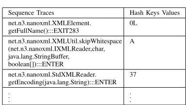
The Sed test data (input/output pairs) consists of a com-mand line which contains 2 main parts: the parameters iden-tifying the operations to be performed and a text file that needs to be modified which therefore forms both part of the input and output. Therefore, the data was transformed in a slightly different way compared to NanoXML and Siena: all input components remained unchanged except the filename (e.g. “../inputs/default.in”) was encoded as the token “<1>” as the file itself contains only the text to be modified. Trying to tokenise the file to be modified (and its modified version) failed to reduce the size of the output sufficiently and so for output part the diff utility (a data comparison tool) was used to calculate the differences between the input text file and its modified form (this process reports how to change the first file to make it match the second file with specific operation that needs to be performed such as “a” for add and “c” for change). The magnitude of the compression achieved by this method is hard to quantify, depending as it does on the file and the modifications, but it typically yielded a much smaller representation of the output data. Table I shows an example of this coding strategy. Each input/output pair was augmented with their associated execution traces in the second study. Sequence traces are often very long, and each entry in a sequence is often a full Java method signature including package name, class name, method name, and parameters (along with their respective long signatures). This required more compression than could be provided by simple tokenisa-tion so the trace compression algorithm developed by Nguyen et al. [23] was used. The algorithm replaces the collections of method sequence entry and exit values with their hash keys, consisting usually of just 1 or 2 characters. It takes into account the occurrence frequency to assign shorter hash keys for entries that are most frequent. Table II shows a sample of sequences for one of collected traces and their hash key values (for space reasons, just 3 sequences are included rather than all sequences

of that trace). The obtained trace from the example in this table

is 0LA37.

Finally all the data items were used in two different studies. In the first study, the input to the classifier was input/output pairs only as a set of vector. This vector is built from two components: input and output. The NanoXML example from Table I was used in the first study and the set of vector was:<FCRSSNRSS, F>. In the second study, the set of vector was extended by adding execution trace. Here the vector is built from three components: input, output and execution trace. So if the NanoXML example from Table I above generated the trace shown in Table II, then the vector would be: <FCRSSNRSS, F, 0LA37>.

TABLE II. EXAMPLECODING OFSEQUENCETRACES

Sequence Traces Hash Keys Values net.n3.nanoxml.XMLElement.

getFullName():::EXIT283

0L

net.n3.nanoxml.XMLUtil.skipWhitespace (net.n3.nanoxml.IXMLReader,char, java.lang.StringBuffer,

boolean[]):::ENTER

A

net.n3.nanoxml.StdXMLReader. getEncoding(java.lang.String):::ENTER

37

. . .

. . .

5) Selection of Labelled and Unlabelled Data: Cross vali-dation was used during the selection of labelled(DL)and un-labelled(DU)data to avoid bias in the choice of data. Different

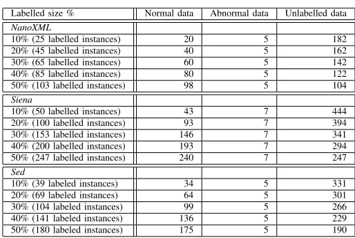
values were set for the size of(DL)in the experiments ranging from 10% to 50% of data (based on a percentage of the number of subject program test cases). The process was repeated so that every input/output pair will appear once in (DL) during training process. Two semi-supervised learning scenarios are explored in this paper: the first is where labels are drawn from both the normal and abnormal classes (i.e. passing and failing tests) and is termedScenario 1, the second is where labels are drawn from just the normal (passing) class (Scenario 2). To try and avoid biasing the results and also to maintain a more realistic scenario, the set of labelled failing cases for scenario 1 was kept deliberately small. Table III shows the labelled data size and class distribution used in all studies for this scenario for all versions of the subject programs.

In practice, it is often difficult to obtain a training data set which covers every possible abnormal behaviour class that can occur in the data so the subset of 5 failing executions was randomly chosen these in turn may appear quite distinct, as one fault may transform the output in may different ways de-pending on the input). The failures to which these correspond for the different versions of NanoXML and Sed are shown in Table IV, and this same abnormal labelled set was used as the size of the normal labelled set grew. For Siena there is just one failure (which again has different manifestations) so all 7 abnormal labels related to this. As mentioned earlier, there may be other ways of obtaining abnormal data such as from previous versions of the software or via seeded faults, and this is something we intend to explore in the future.

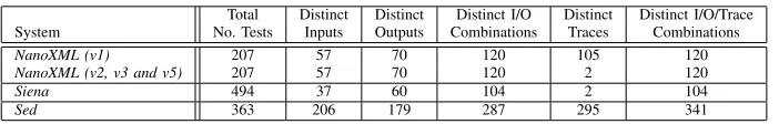
of the machine learning algorithms employed. Table V shows for each system3 the number of test cases followed by the number of distinct inputs, outputs, input-output combinations, traces, and input-output-trace information. We will return to this table in the discussion of the results.

TABLE III. LABELLED TRAINING DATA SET SIZES AND CLASS DISTRIBUTION FOR ALL SYSTEMS FOR SCENARIO1

Labelled size % Normal data Abnormal data Unlabelled data NanoXML

10% (25 labelled instances) 20 5 182 20% (45 labelled instances) 40 5 162 30% (65 labelled instances) 60 5 142 40% (85 labelled instances) 80 5 122 50% (103 labelled instances) 98 5 104 Siena

10% (50 labelled instances) 43 7 444 20% (100 labelled instances) 93 7 394 30% (153 labelled instances) 146 7 341 40% (200 labelled instances) 193 7 294 50% (247 labelled instances) 240 7 247 Sed

10% (39 labeled instances) 34 5 331 20% (69 labeled instances) 64 5 301 30% (104 labeled instances) 99 5 266 40% (141 labeled instances) 136 5 229 50% (180 labeled instances) 175 5 190

TABLE IV. ABNORMALLYLABELLEDDATA FOR FORSCENARIO1 Version No. Labelled Failures (number of instances) NanoXML

Version 1 F1 (5) Version 2 F6 (3) and F7 (2) version 3 F6 (3) and F7 (2) Version 5 F1 (2) and F2 (3) Siena

Version 2, 4 and 6 Single Failure (7) Sed

Version 5 F3 (5)

C. Evaluation

To evaluate the performance of semi-supervised learning

algorithms we use the F-measure – a combination measure

of PrecisionandRecall(widely used measures in information science domain). These measures in turn rely on the concepts of true positives (TP), false positives (FP) and false negatives (FN) which are defined in this context as follows:

TP: A failing test result classified as failing test FP: A passing test result classified as failing test FN: A failing test result classified as passing test Precision is defined as the ratio of correctly classified failures to the total number of true positive (correctly classified fail-ures) and false positive (incorrectly classified passing tests):

P recision(P R) = (T P)

(T P+F P) (1)

Recall is the ratio of correctly classified failures to the total number of true positive (correctly classified failures) and false negative (incorrectly classified failing tests):

Recall(RE) = (T P)

(T P +F N) (2)

3_{Versions 2, 3 and 5 of NanoXML are broadly similar in this respect and}

have been grouped together

The Fmeasure the harmonic mean of precision and recall -combines these two as follows:

F−measure= 2(P R×RE)

(P R+RE) (3)

In all cases these values are calculated purely on the unlabelled data instances - (DU) in the section above.

D. Tools and Configuration

A collective classification package (release 2015.2.27)4for semi-supervised learning in WEKA5_{(release 3-6-12) was used}

in the experiments. The maximum number of iterations in self-training and co-self-training is set to 80, and to 30 for co-EM in the experiments (as used in [31]). Default values for all other parameters (except the iteration parameter) were used as given in their implementation. The Daikon configuration employed was the most recent version and the same as that used in other experiments [21], [23].

V. EXPERIMENTALRESULTS ANDDISCUSSION

In this section, the results obtained from using semi-supervised learning classifiers (self-training, co-training and co-EM) on the three subject programs described in Section IV are presented. Two separate studies were performed using two kinds of execution data: firstly just input/output pairs, and secondly input/output pairs augmented with execution traces and in addition the two semi-supervised labelling scenarios were explored (section III-A).

A. Study 1: Test Result Classification Based on Input/Output Pairs

1) Scenario 1: Labelling subsets of both passing (normal) and failing (abnormal) tests: For the first study the classifiers were built using just the input and output of the test cases that were provided with the three systems. In this scenario the clas-sifiers were trained on a small set of labelled instances of the normal behaviour class (in this case, passing executions) and a few instances for abnormal behaviour (failing executions). The rest of the data were unlabelled instances of input output pairs which the classifiers iteratively categorised during the learning process.

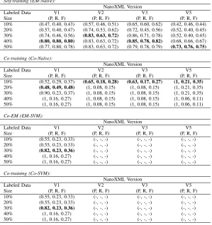
Tables VI and VII show, for NanoXML and for Siena and Sed respectively, the results of applying semi-supervised learn-ing with increaslearn-ing numbers of labelled samples. The figures reported are the average values obtained from employing cross validation to reduce the potential bias created by the choice of the labelled data items (see section IV-B5). The first column (size) defines the number of labelled data items in the training sets as a percentage of the total number of test cases. The subsequent columns identify the version number of the subject programs with (P, R, F) referring to the average values of Precision, Recall and F-measure (see sectionIV-C) with the best results in each column highlighted in bold.

For NanoXML the self-training method (Na¨ıve Bayes with EM) performed well over all versions, achieving an average

TABLE V. DOMAINSIZE FOR THETHREESYSTEMS

Total Distinct Distinct Distinct I/O Distinct Distinct I/O/Trace System No. Tests Inputs Outputs Combinations Traces Combinations

NanoXML (v1) 207 57 70 120 105 120

NanoXML (v2, v3 and v5) 207 57 70 120 2 120

Siena 494 37 60 104 2 104

Sed 363 206 179 287 295 341

F-measure of 0.5 when only 10% of the data (just 25 items) was labelled. However, to achieve the better results it would be necessary to label between 30-50% of the data. Co-training using Na¨ıve Bayes performed far less well, and more notably didn’t really improve as the size of the labelled training set increased. Even more disappointing are the results for co-EM and co-training with SVM: the performance for version 1 of NanoXML is identical for both algorithms but let down by poor recall values, but for versions 2, 3 and 5 the recall was zero most of the time as no failures were detected (indicated by a ‘-’ n the results tables) and something that needs to be explored further).

The performance of Na¨ıve Bayes with EM on NanoXML is encouraging, particularly considering the number of input and output combinations that need to be classified (see Table V). Given that there are 120 distinct input-output pairs it is also to be expected that the performance improves when the 30-50% bracket is reached – at this point between 60-100 data items will have been labelled and chances are that this will have covered the majority of the distinct combinations. It might be expected that as more cases get labelled so the accuracy would increase but this is not always the case, especially for some of the other algorithms. Looking at these cases it appears that initially many results were classified as fail (some correctly, some not). As more data gets labelled several of these fail results were turned into passes - some correctly but some not - due to the influence of one label (they may match a labelled passing input for example). This impacts on precision and recall as the FP value will drop as will the TP value which means that precision increases (negatively impacted by FP) but recall decreases (negatively impacted by TP). By adding in more data in the form of traces it is anticipated that this undue influence from one component will diminish.

A similar pattern of results can be seen from the data for Siena – the semi-supervised learning techniques did not perform well in all versions. Remember that the versions of Siena contain just the one fault, so all failures correspond to the same fault (but which will have different manifestations). As with NanoXML the best F-measure values are achieved with self-training (Na¨ıve Bayes with EM) but unlike NanoXML there was no increase in performance as the proportion of labelled data increased. This feature is something of a surprise as in comparison to NanoXML the number of input-output combinations for Siena is relatively small (104 - see TableV). With nearly 500 test cases for the system the expectation would be for the majority of these combinations would be included by the time that 30% of the data was labelled but this seemed to have no impact. This may be down to the either the choice of abnormal cases or the fact that the increase in the number of tests means the data becomes very imbalanced. The results for the other approaches are generally poor, and when not zero are too low to be considered usable.

The results for Sed in some ways also reflect those for the other two systems. The best results are achieved using Na¨ıve Bayes with EM but at the low level of labelling these are quite weak. It is only when around 30% of the data is labelled that these begin to become acceptable. This is perhaps to be expected as Sed had the most fragmented input-output profile of all the systems (287 in total - see TableV).

2) Scenario 2: Labelling subsets of only passing (normal) tests: In the second scenario classifiers were trained on a small set of labelled instances for normal behaviour class (passing executions) alone, with the remaining data being unlabelled instances (an unknown class for the classifier during the training process). The same set of learning strategies were explored but none of approaches performed well enough to warrant reporting in more detail. The majority of the time the trained classifiers were able to classify passing (normal) execution data correctly but miss-classified failing (abnormal) execution data, labelling it as normal data instead.

B. Study 2: Test Result Classification Based on Input/Output Pairs Augmented with Execution Traces

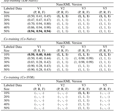
1) Scenario 1: Labelling subsets of both passing (normal) and failing (abnormal) tests: For this second study the input data for the semi-supervised learning strategies consisted of the input/output pairs used in the first study augmented with their execution traces. In both cases the data are encoded as described in section IV-B4 to reduce them to a manageable size (the trace data in particular). This change aside, all other aspects - semi-supervised learning algorithms, subject programs, proportions of labelled data explored - are identical to the first study.

TABLE VI. AVERAGEPRECISION(P), RECALL(R)ANDF-MEASURE(F) RESULTS FORNANOXMLUSINGSEMI-SUPERVISEDLEARNING ON

INPUT/OUTPUTPAIRS ANDTRAINED ONNORMAL ANDABNORMALCASES

Self-training (EM-Na¨ıve):

NanoXML Version

Labeled Data V1 V2 V3 V5

Size (P, R, F) (P, R, F) (P, R, F) (P, R, F) 10% (0.47, 0.40, 0.43) (0.57, 0.46, 0.51) (0.65, 0.60, 0.62) (0.42, 0.46, 0.44) 20% (0.57, 0.40, 0.47) (0.74, 0.53, 0.62) (0.72, 0.45, 0.56) (0.52, 0.40, 0.45) 30% (0.74, 0.46, 0.56) (0.83, 0.63, 0.72) (0.86, 0.71, 0.78) (0.52, 0.40, 0.45) 40% (0.80, 0.80, 0.80) (0.83, 0.63, 0.72) (0.85, 0.78, 0.82) (0.68, 0.66, 0.67) 50% (0.77, 0.80, 0.78) (0.83, 0.63, 0.72) (0.79, 0.78, 0.79) (0.73, 0.76, 0.75)

Co-training (Co-Na¨ıve):

NanoXML Version

Labeled Data V1 V2 V3 V5

Size (P, R, F) (P, R, F) (P, R, F) (P, R, F) 10% (0.52, 0.29, 0.37) (0.65, 0.18, 0.28) (0.63, 0.17, 0.27) (1, 0.21, 0.35) 20% (0.48, 0.49, 0.48) (1, 0.08, 0.15) (1, 0.08, 0.15) (1, 0.21, 0.35) 30% (0.90, 0.23, 0.37) (1, 0.08, 0.15) (1, 0.08, 0.15) (1, 0.21, 0.35) 40% (1, 0.16, 0.27) (1, 0.08, 0.15) (1, 0.08, 0.15) (1, 0.06, 0.11) 50% (1, 0.16, 0.27) (1, 0.08, 0.15) (1, 0.08, 0.15) (1, 0.06, 0.11)

Co-EM (EM-SVM):

NanoXML Version

Labeled Data V1 V2 V3 V5

Size (P, R, F) (P, R, F) (P, R, F) (P, R, F) 10% (0.55, 0.23, 0.33) (-, -, -) (-, -, -) (-, -, -) 20% (0.55, 0.23, 0.33) (-, -, -) (-, -, -) (-, -, -) 30% (0.82, 0.23, 0.36) (-, -, -) (-, -, -) (-, -, -) 40% (1, 0.16, 0.27) (-, -, -) (-, -, -) (-, -, -) 50% (1, 0.16, 0.27) (-, -, -) (-, -, -) (-, -, -)

Co-training (Co-SVM):

NanoXML Version

Labeled Data V1 V2 V3 V5

Size (P, R, F) (P, R, F) (P, R, F) (P, R, F) 10% (0.55, 0.23, 0.33) (-, -, -) (-, -, -) (-, -, -) 20% (0.55, 0.23, 0.33) (-, -, -) (-, -, -) (-, -, -) 30% (0.82, 0.23, 0.36) (-, -, -) (-, -, -) (-, -, -) 40% (1, 0.16, 0.27) (-, -, -) (-, -, -) (-, -, -) 50% (1, 0.16, 0.27) (-, -, -) (-, -, -) (-, -, -)

the performance is notably better than the results achieved from classifying the input-output data alone without the execution trace information.

Co-training using Na¨ıve Bayes displays a very similar pattern although the improvement observable in version 1 for self-training is absent. Co-training with SVM did not perform well on any versions with the exception of version 3 (it is unclear why similar results should be have been achieved for versions 2 and 5). The results for co-EM were particularly poor and have been omitted from the table.

The results for Siena for all techniques (with the exception again of co-EM) are universally good, accurately classifying the passing and failing executions with 100% accuracy based on just the smallest labelling proportion. Again, this is for exactly the same reasons as versions 2,3 and 5 of NanoXML – the passing and failing executions are perfectly separable based on the execution traces alone. This trace pattern was entirely unknown at the time the two systems were selected and not something that was either expected or planned for.

Sed displays a very similar pattern of results to those achieved using input-output pairs alone. Indeed the inclusion of execution traces appears to have practically no impact on the results. It has already been observed that Sed has the most fragmented input-output combination, and combined with its 295 distinct traces gives a 341 distinct input-output-trace combinations. For cases such as this it is clear that other information needs to be introduced to the classifier algorithms

such as execution time or summary information relating to traces (e.g. number of unique methods, nesting pattern etc.) and is something we intend to explore in future.

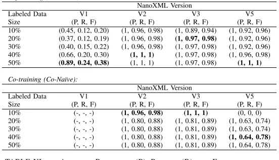
2) Scenario 2: Labelling subsets of only passing (normal) tests: For this part of the study the data used was as for the first scenario - input/output pairs augmented with their execution traces - but only a normal (passing execution) subset of the data was labelled. The results are shown in Tables X and XI and display a similar, but slightly less effective, pattern to scenario 1.

TABLE VII. AVERAGEPRECISION(P), RECALL(R)ANDF-MEASURE

(F) RESULTS FORSIENA ANDSED USINGSEMI-SUPERVISEDLEARNING ONINPUT/OUTPUTPAIRS ANDTRAINED ONNORMAL ANDABNORMAL

CASES

Self-training (EM-Na¨ıve):

Siena Version Sed Version Labeled Data V2 Labeled Data V5 Size (P, R, F) Size (P, R, F) 10% (0.19, 0.60, 0.28) 10% (1, 0.10, 0.19) 20% (0.10, 0.23, 0.13) 20% (1, 0.10, 0.19) 30% (0.09, 0.20, 0.12) 30% (0.39, 0.86, 0.54) 40% (0.09, 0.20, 0.12) 40% (0.39, 0.86, 0.54) 50% (0.09, 0.20, 0.12) 50% (0.39, 0.86, 0.54)

Co-training (Co-Na¨ıve):

Siena Version Sed Version Labeled Data V2 Labeled Data V5 Size (P, R, F) Size (P, R, F) 10% (0.09, 0.21, 0.13) 10% (1, 0.04, 0.08) 20% (0.37, 0.10, 0.16) 20% (1, 0.04, 0.08) 30% (0.16, 0.03, 0.05) 30% (1, 0.04, 0.08) 40% (0.10, 0.23, 0.14) 40% (0.85, 0.36, 0.51) 50% (0.09, 0.21, 0.13) 50% (0.85, 0.36, 0.51)

Co-training (Co-SVM):

Siena Version Sed Version Labeled Data V2 Labeled Data V5 Size (P, R, F) Size (P, R, F) 10% (0.11, 0.15, 0.13) 10% (-, -, -) 20% (-, -, -) 20% (-, -, -) 30% (-, -, -) 30% (-, -, -) 40% (-, -, -) 40% (-, -, -) 50% (-, -, -) 50% (-, -, -)

TABLE VIII. AVERAGEPRECISION(P), RECALL(R)ANDF-MEASURE

(F) RESULTS FORNANOXMLUSINGSEMI-SUPERVISEDLEARNING ON

INPUT/OUTPUTPAIRSAUGMENTED WITHEXECUTIONTRACES AND

TRAINED ONNORMAL ANDABNORMALCASES

Self-training (EM-Na¨ıve):

NanoXML Version

Labeled Data V1 V2 V3 V5

Size (P, R, F) (P, R, F) (P, R, F) (P, R, F) 10% (0.50, 0.41, 0.45) (1, 1, 1) (1, 1, 1) (1, 1, 1) 20% (0.47, 0.47, 0.47) (1, 1, 1) (1, 1, 1) (1, 1, 1) 30% (0.70, 0.94, 0.80) (1, 1, 1) (1, 1, 1) (1, 1, 1) 40% (0.86, 0.94, 0.90) (1, 1, 1) (1, 1, 1) (1, 1, 1) 50% (0.94, 0.94, 0.94) (1, 1, 1) (1, 1, 1) (1, 1, 1)

Co-training (Co-Na¨ıve):

NanoXML Version

Labeled Data V1 V2 V3 V5

Size (P, R, F) (P, R, F) (P, R, F) (P, R, F) 10% (0.50, 0.40, 0.44) (1, 1, 1) (1, 1, 1) (1, 1, 1) 20% (0.50, 0.40, 0.44) (1, 1, 1) (1, 0.98, 0.99) (1, 1, 1) 30% (0.83, 0.28, 0.42) (1, 1, 1) (1, 0.98, 0.99) (1, 1, 1) 40% (0.90, 0.28, 0.43) (1, 1, 1) (1, 1, 1) (1, 1, 1) 50% (0.90, 0.28, 0.43) (1, 1, 1) (1, 1, 1) (1, 1, 1)

Co-training (Co-SVM):

NanoXML Version

Labeled Data V1 V2 V3 V5

Size (P, R, F) (P, R, F) (P, R, F) (P, R, F) 10% (-, -, -) (-, -, -) (1, 1, 1) (-, -, -) 20% (-, -, -) (-, -, -) (1, 1, 1) (-, -, -) 30% (-, -, -) (-, -, -) (1, 1, 1) (-, -, -) 40% (-, -, -) (-, -, -) (1, 1, 1) (-, -, -) 50% (-, -, -) (-, -, -) (1, 1, 1) (-, -, -)

The results for Siena (table X) show that both self-training (Na¨ıve Bayes with EM) and co-training (Na¨ıve Bayes) methods have extremely performed well, again due to the very infor-mative execution traces. Self-training was able to detect all failures with all labelled sample sizes on all versions and co-training produced a similar set of results with the exception of the smallest (10%) labelling proportion . Co-training with SVM and co-EM again did not perform well for Siena either

TABLE IX. AVERAGEPRECISION(P), RECALL(R)ANDF-MEASURE

(F) RESULTS FORSIENA ANDSED USINGSEMI-SUPERVISEDLEARNING ONINPUT/OUTPUTPAIRSAUGMENTED WITHEXECUTIONTRACES AND

TRAINED ONNORMAL ANDABNORMALCASES

Self-training (EM-Na¨ıve):

Siena Version Sed Version Labeled Data V2 Labeled Data V5 Size (P, R, F) Size (P, R, F) 10% (1, 1, 1) 10% (1, 0.10, 0.19) 20% (1, 1, 1) 20% (1, 0.10, 0.19) 30% (1, 1, 1) 30% (0.39, 0.86, 0.54) 40% (1, 1, 1) 40% (0.39, 0.86, 0.54) 50% (1, 1, 1) 50% (0.39, 0.86, 0.54)

Co-training (Co-Na¨ıve):

Siena Version Sed Version Labeled Data V2 Labeled Data V5 Size (P, R, F) Size (P, R, F) 10% (1, 1, 1) 10% (1, 0.07, 0.14) 20% (1, 1, 1) 20% (1, 0.07, 0.14) 30% (1, 1, 1) 30% (1, 0.07, 0.14) 40% (1, 1, 1) 40% (0.39, 0.84, 0.53) 50% (1, 1, 1) 50% (0.39, 0.84, 0.53)

Co-training (Co-SVM):

Siena Version Sed Version Labeled Data V2 Labeled Data V5 Size (P, R, F) Size (P, R, F) 10% (1, 1, 1) 10% (-, -, -) 20% (1, 1, 1) 20% (-, -, -) 30% (1, 1, 1) 30% (-, -, -) 40% (1, 1, 1) 40% (-, -, -) 50% (1, 1, 1) 50% (-, -, -)

Co-EM (EM-SVM):

Siena Version Sed Version Labeled Data V2 Labeled Data V5 Size (P, R, F) Size (P, R, F) 10% (-, -, -) 10% (1, 0.07, 0.14) 20% (-, -, -) 20% (1, 0.07, 0.14) 30% (-, -, -) 30% (1, 0.07, 0.14) 40% (-, -, -) 40% (1, 0.07, 0.14) 50% (-, -, -) 50% (1, 0.07, 0.14)

and the results for these have been omitted.

Again Sed proved to be the most challenging system and for Na¨ıve Bayes with EM did not display any acceptable results until at least 30% of the data was labelled (again attributable to the fragmentation). Co-training (Na¨ıve Bayes) displayed a similar performance but was able to produce results even with the smallest level of labelling. Even though the results for this approach are not as accurate as the previous scenario, the absence of any labelled failing inputs makes this an interesting outcome.

VI. THREATS TOVALIDITY

The clear issue concerning the external validity of this work is the generalizability of our results: the findings so far are limited to three subject programs which cannot be said to form a representative set, even though they are non-trivial real-world Java and C systems of a reasonable size containing real faults. The failure rates for both systems may also not be representative, as may be the test cases (although these were created independently via collaboration between the SIR and the subject systems’ developers).

TABLE X. AVERAGEPRECISION(P), RECALL(R)ANDF-MEASURE

(F) RESULTS FORNANOXMLUSINGSEMI-SUPERVISEDLEARNING ON

INPUT/OUTPUTPAIRSAUGMENTED WITHEXECUTIONTRACES AND

TRAINED ONNORMALCASESALONE

Self-training (EM-Na¨ıve):

NanoXML Version

Labeled Data V1 V2 V3 V5

Size (P, R, F) (P, R, F) (P, R, F) (P, R, F) 10% (0.45, 0.12, 0.20) (1, 0.96, 0.98) (1, 0.89, 0.94) (1, 0.92, 0.96) 20% (0.37, 0.12, 0.19) (1, 0.96, 0.98) (1, 0.97, 0.98) (1, 0.92, 0.96) 30% (0.40, 0.15, 0.22) (1, 0.96, 0.98) (1, 0.97, 0.98) (1, 0.92, 0.96) 40% (0.66, 0.20, 0.30) (1, 1, 1) (1, 0.97, 0.98) (1, 0.96, 0.98) 50% (0.89, 0.24, 0.38) (1, 1, 1) (1, 0.97, 0.98) (1, 1, 1)

Co-training (Co-Na¨ıve):

NanoXML Version

Labeled Data V1 V2 V3 V5

Size (P, R, F) (P, R, F) (P, R, F) (P, R, F) 10% (-, -, -) (1, 0.96, 0.98) (1, 1, 1) (0, 0, 0) 20% (-, -, -) (1, 0.80, 0.88) (1, 0.81, 0.89) (1, 0.63, 0.74) 30% (-, -, -) (1, 0.80, 0.88) (1, 0.81, 0.89) (1, 0.63, 0.74) 40% (-, -, -) (1, 0.80, 0.88) (1, 0.81, 0.89) (1, 0.64, 0.78) 50% (-, -, -) (1, 0.80, 0.88) (1, 0.81, 0.89) (1, 0.64, 0.78)

TABLE XI. AVERAGEPRECISION(P), RECALL(R)ANDF-MEASURE

(F) RESULTS FORSIENA ANDSED USINGSEMI-SUPERVISEDLEARNING ONINPUT/OUTPUTPAIRSAUGMENTED WITHEXECUTIONTRACES AND

TRAINED ONNORMALCASESALONE

Self-training (EM-Na¨ıve):

Siena Version Sed Version Labeled Data V2 Labeled Data V5 Size (P, R, F) Size (P, R, F) 10% (1, 1, 1) 10% (-, -, -) 20% (1, 1, 1) 20% (-, -, -) 30% (1, 1, 1) 30% (0.39, 0.45, 0.42) 40% (1, 1, 1) 40% (0.33, 0.56, 0.42) 50% (1, 1, 1) 50% (0.41, 0.68, 0.51)

Co-training (Co-Na¨ıve):

Siena Version Sed Version Labeled Data V2 Labeled Data V5 Size (P, R, F) Size (P, R, F) 10% (1, 0.81, 0.89) 10% (0.38, 0.28, 0.33) 20% (1, 1, 1) 20% (0.36, 0.25, 0.30) 30% (1, 1, 1) 30% (0.43, 0.39, 0.41) 40% (1, 1, 1) 40% (0.40, 0.45, 0.42) 50% (1, 1, 1) 50% (0.42, 0.48, 0.45)

automatically in the reminder of the data set. The coding scheme for execution traces was the same algorithm used by [23] and also has no information about whether a trace is associated with a passing or failing execution.

VII. SUMMARY, CONCLUSIONS ANDFUTUREWORK

In this paper we present an empirical study, which demon-strates the potential of semi-supervised learning techniques to support the construction of automated test oracles by classi-fying passing and failing outputs. We perform three different studies and also examine two different scenarios associated with semi-supervised learning techniques: labelling both nor-mal (passing) and abnornor-mal (failing) tests, and labelling nornor-mal (passing) tests alone. Just input/output pairs were used as input to the learning algorithms in the first study, and then augmented with execution traces in the second.

The main findings from this study may be summarised as follows:

• From the algorithms investigated Na¨ıve Bayes with EM and co-training using Na¨ıve Bayes proved to be the most consistent performers. These approaches have been shown to perform well in the area of document classification where all of the data sets are textual (as in this study) which may go some way towards explaining the reason for their performance in relation to the much poorer one of Support Vector Machines with the co-EM and co-training methods. • Considering just input-output pairs with positive labels

(passing cases) alone yielded very poor results and is not worth exploring further.

• The results for input-output pairs with positive and negative labels (a subset of passing cases and a small number of failing ones) were variable: encouraging for NanoXML, acceptable for Sed but disappointing for Siena. This result was a surprise given that the profile of the system is far less fragmented than Sed, but could be attributable to a data imbalance problem - something that needs explored in the future. • Adding in execution trace data can help enormously.

This is not really unexpected given that more informa-tion is being supplied to the algorithm, but even when very fragmented they improve the accuracy once a fair proportion of the data is labelled. In extreme cases the impact is dramatic (leading to a perfect classifier on from a very small subset of labelled data) but we assume that these are relatively rare instances. • Using input-output pairs and execution traces with just

positive labels worked well when the number of traces is small) but otherwise didn’t perform as well as when a small number of failing inputs are provided.

Even though these results are preliminary we believe the findings from this study have important implications for the practical use of this technique: when checking the test results from a system a developer need only examine a relatively small proportion of these and use this information to train a learning algorithm to classify the remainder. This has the potential to improve the efficiency and reduce the cost and tedium of manually checking large volumes of test results. Future research will be devoted to further empirical investigation of the effectiveness of our approach corroborate the findings and to increase their external validity, particularly by exploring a wider range of programs and faults.

All the data for the study is available at

REFERENCES

[1] G. Fraser and A. Arcuri, “Evosuite: Automatic test suite generation for object-oriented software,” in Proceedings of the 19th ACM SIGSOFT Symposium and the 13th European Conference on Foundations of Software Engineering, ser. ESEC/FSE ’11. New York, NY, USA: ACM, 2011, pp. 416–419. [Online]. Available: http://doi.acm.org/10.1145/2025113.2025179

[2] E. Barr, M. Harman, P. McMinn, M. Shahbaz, and S. Yoo, “The oracle problem in software testing: A survey,” Software Engineering, IEEE Transactions on, vol. 41, no. 5, pp. 507–525, May 2015.

[3] R.-K. Doong and P. G. Frankl, “The astoot approach to testing object-oriented programs,” ACM Trans. Softw. Eng. Methodol., vol. 3, no. 2, pp. 101–130, Apr. 1994. [Online]. Available: http://doi.acm.org/10.1145/192218.192221

[4] C. Pacheco and M. D. Ernst, “Randoop: Feedback-directed random testing for java,” inCompanion to the 22Nd ACM SIGPLAN Conference on Object-oriented Programming Systems and Applications Companion, ser. OOPSLA ’07. New York, NY, USA: ACM, 2007, pp. 815–816. [Online]. Available: http://doi.acm.org/10.1145/1297846.1297902 [5] L. Baresi and M. Young, “Test oracles,” Tech. Rep., 2001.

[6] M. Pezz`e and C. Zhang, “Automated test oracles: A survey,” in

Advances in Computers. Elsevier, 2015, vol. 95, pp. 1–48.

[7] B. P. Miller, L. Fredriksen, and B. So, “An empirical study of the reliability of unix utilities,”Commun. ACM, vol. 33, no. 12, pp. 32–44, Dec. 1990. [Online]. Available: http://doi.acm.org/10.1145/96267.96279 [8] Z. Q. Zhou, S. Zhang, M. Hagenbuchner, T. H. Tse, F.-C. Kuo, and T. Y. Chen, “Automated functional testing of online search services,”

Softw. Test. Verif. Reliab., vol. 22, no. 4, pp. 221–243, Jun. 2012. [Online]. Available: http://dx.doi.org/10.1002/stvr.437

[9] W. Dickinson, D. Leon, and A. Podgurski, “Finding failures by cluster analysis of execution profiles,” inSoftware Engineering, 2001. ICSE 2001. Proceedings of the 23rd International Conference on, May 2001, pp. 339–348.

[10] ——, “Pursuing failure: The distribution of program failures in a profile space,” in Proceedings of the 8th European Software Engineering Conference Held Jointly with 9th ACM SIGSOFT International Symposium on Foundations of Software Engineering, ser. ESEC/FSE-9. New York, NY, USA: ACM, 2001, pp. 246–255. [Online]. Available: http://doi.acm.org/10.1145/503209.503243

[11] A. Rafig and M. Roper, “Building test oracles by clustering failures,” in Proceedings of the 10th International Workshop on Automation of Software Test, ser. AST 2015. IEEE, 2015.

[12] S. Yoo, M. Harman, P. Tonella, and A. Susi, “Clustering test cases to achieve effective & scalable prioritisation incorporating expert knowl-edge,” inProceedings of International Symposium on Software Testing and Analysis (ISSTA 2009). ACM Press, July 2009, pp. 201–211. [13] A. Podgurski, D. Leon, P. Francis, W. Masri, M. Minch, J. Sun,

and B. Wang, “Automated support for classifying software failure reports,” in Proceedings of the 25th International Conference on Software Engineering, ser. ICSE ’03. Washington, DC, USA: IEEE Computer Society, 2003, pp. 465–475. [Online]. Available: http://dl.acm.org/citation.cfm?id=776816.776872

[14] J. F. Bowring, J. M. Rehg, and M. J. Harrold, “Active learning for automatic classification of software behavior,” in Proceedings of the 2004 ACM SIGSOFT International Symposium on Software Testing and Analysis, ser. ISSTA ’04. New York, NY, USA: ACM, 2004, pp. 195– 205. [Online]. Available: http://doi.acm.org/10.1145/1007512.1007539 [15] M. Vanmali, M. Last, and A. Kandel, “Using a neural network

in the software testing process,” International Journal of Intelligent Systems, vol. 17, no. 1, pp. 45–62, 2002. [Online]. Available: http://dx.doi.org/10.1002/int.1002

[16] L. Briand, “Novel applications of machine learning in software test-ing,” in Quality Software, 2008. QSIC ’08. The Eighth International Conference on, Aug 2008, pp. 3–10.

[17] D. Lo, H. Cheng, J. Han, S.-C. Khoo, and C. Sun, “Classification of software behaviors for failure detection: A discriminative pattern mining approach,” in Proceedings of the 15th ACM SIGKDD International Conference on Knowledge Discovery and Data Mining, ser. KDD ’09. New York, NY, USA: ACM, 2009, pp. 557–566. [Online]. Available: http://doi.acm.org/10.1145/1557019.1557083

[18] C. Yilmaz and A. Porter, “Combining hardware and software instrumentation to classify program executions,” in Proceedings of the Eighteenth ACM SIGSOFT International Symposium on Foundations of Software Engineering, ser. FSE ’10. New York, NY, USA: ACM, 2010, pp. 67–76. [Online]. Available: http://doi.acm.org/10.1145/1882291.1882304

[19] S. Shahamiri, W. Wan-Kadir, S. Ibrahim, and S. Hashim, “Artificial neural networks as multi-networks automated test oracle,”Automated Software Engineering, vol. 19, no. 3, pp. 303–334, 2012. [Online]. Available: http://dx.doi.org/10.1007/s10515-011-0094-z

[20] L. Mariani and F. Pastore, “Automated identification of failure causes in system logs,” inSoftware Reliability Engineering, 2008. ISSRE 2008. 19th International Symposium on, Nov 2008, pp. 117–126.

[21] M. D. Ernst, J. H. Perkins, P. J. Guo, S. McCamant, C. Pacheco, M. S. Tschantz, and C. Xiao, “The daikon system for dynamic detection of likely invariants,” Sci. Comput. Program., vol. 69, no. 1-3, pp. 35–45, Dec. 2007. [Online]. Available: http://dx.doi.org/10.1016/j.scico.2007.01.015

[22] I. Beschastnikh, Y. Brun, S. Schneider, M. Sloan, and M. D. Ernst, “Leveraging existing instrumentation to automatically infer invariant-constrained models,” in Proceedings of the 19th ACM SIGSOFT Symposium and the 13th European Conference on Foundations of Software Engineering, ser. ESEC/FSE ’11. New York, NY, USA: ACM, 2011, pp. 267–277. [Online]. Available: http://doi.acm.org/10.1145/2025113.2025151

[23] C. D. Nguyen, A. Marchetto, and P. Tonella, “Automated oracles: An empirical study on cost and effectiveness,” inProceedings of the 2013 9th Joint Meeting on Foundations of Software Engineering, ser. ESEC/FSE 2013. New York, NY, USA: ACM, 2013, pp. 136–146. [Online]. Available: http://doi.acm.org/10.1145/2491411.2491434 [24] V. Chandola, A. Banerjee, and V. Kumar, “Anomaly detection: A

survey,”ACM Comput. Surv., vol. 41, no. 3, pp. 15:1–15:58, Jul. 2009. [Online]. Available: http://doi.acm.org/10.1145/1541880.1541882 [25] D. Dasgupta and F. Nino, “A comparison of negative and positive

selection algorithms in novel pattern detection,” inSystems, Man, and Cybernetics, 2000 IEEE International Conference on, vol. 1, 2000, pp. 125–130 vol.1.

[26] D. Dasgupta and N. Majumdar, “Anomaly detection in multidimensional data using negative selection algorithm,” inEvolutionary Computation, 2002. CEC ’02. Proceedings of the 2002 Congress on, vol. 2, 2002, pp. 1039–1044.

[27] R. Fujimaki, “An approach to spacecraft anomaly detection problem using kernel feature space,” in in Proc. PAKDD-2005: Ninth Pacific-Asia Conference on Knowledge Discovery and Data Mining. ACM Press, 2005.

[28] K. Nigam, A. K. McCallum, S. Thrun, and T. Mitchell, “Text classification from labeled and unlabeled documents using em,”Mach. Learn., vol. 39, no. 2-3, pp. 103–134, May 2000. [Online]. Available: http://dx.doi.org/10.1023/A:1007692713085

[29] A. Blum and T. Mitchell, “Combining labeled and unlabeled data with co-training,” in Proceedings of the Eleventh Annual Conference on Computational Learning Theory, ser. COLT’ 98. New York, NY, USA: ACM, 1998, pp. 92–100. [Online]. Available: http://doi.acm.org/10.1145/279943.279962

[30] K. Nigam and R. Ghani, “Analyzing the effectiveness and applicability of co-training,” inProceedings of the Ninth International Conference on Information and Knowledge Management, ser. CIKM ’00. New York, NY, USA: ACM, 2000, pp. 86–93. [Online]. Available: http://doi.acm.org/10.1145/354756.354805

[31] Y. Guo, X. Niu, and H. Zhang, “An extensive empirical study on semi-supervised learning,” in Data Mining (ICDM), 2010 IEEE 10th International Conference on, Dec 2010, pp. 186–195.

[32] H. Do, S. Elbaum, and G. Rothermel, “Supporting controlled experimentation with testing techniques: An infrastructure and its potential impact,”Empirical Softw. Engg., vol. 10, no. 4, pp. 405–435, Oct. 2005. [Online]. Available: http://dx.doi.org/10.1007/s10664-005-3861-2