A Direct Memetic Approach to the Solution of
Multi-Objective Optimal Control Problems
Massimiliano Vasile
Department of Mechanical & Aerospace Engineering University of Strathclyde
Glasgow, UK
Email: [email protected]
Lorenzo Ricciardi
Department of Mechanical & Aerospace Engineering University of Strathclyde
Glasgow, UK
Email: [email protected]
Abstract—This paper proposes a memetic direct transcription algorithm to solve Multi-Objective Optimal Control Problems (MOOCP). The MOOCP is first transcribed into a Non-linear Programming Problem (NLP) with Direct Finite Elements in Time (DFET) and then solved with a particular formulation of the Multi Agent Collaborative Search (MACS) framework. Multi Agent Collaborative Search is a memetic algorithm in which a population of agents combines local search heuristics, exploring the neighbourhood of each agent, with social actions exchanging information among agents. A collection of all Pareto optimal solutions is maintained in an archive that evolves towards the Pareto set. In the approach proposed in this paper, individualistic actions run a local search, from random points within the neighbourhood of each agent, solving a normalised Pascoletti-Serafini scalarisation of the multi-objective NLP problem. Social actions, instead, solve a bi-level problem in which the lower level handles only the constraint equations while the upper level handles only the objective functions. The proposed approach is tested on the multi-objective extensions of two well-known optimal control problems: the Goddard Rocket problem, and the maximum energy orbit rise problem.
I. INTRODUCTION
In many practical cases in which a dynamical system needs to be controlled, it is desirable to generate multiple alternative solutions that are optimal with respect to a number of conflict-ing cost functions. In the literature, few approaches have been proposed to tackle multi-objective optimal control problems: in Coverstone et al. [1] the authors combined Genetic Algorithms and optimal control theory in a dual loop algorithm. In the outer loop, NSGAII was generating vectors of co-states and times of flight. For each set, the inner loop was solving a single objective optimal control problem with given time of flight, minimising the propellant consumption. In Ober-Blobaum et al. [2] a direct transcription approach is used, coupled with an approach that scalarises the multi-objective vector along directions pointing at predefined unreachable points in the criteria space. Each scalar problem is then solved with a standard NLP solver. In [3] a similar approach is proposed that uses a smoothed version of Tchebycheff scalarisation to scalarise the MOO problem. In [4] the authors proposed a dual loop algorithm in which the outer loop solves a multi-objective problem handling a set of categorical variables and the inner loop solves a set of single objective constrained optimal control problems using Monotonic Basin Hopping.
This paper proposes a memetic approach to find a set of Pareto optimal control policies that satisfy a set of dynamic and algebraic constraints. The memetic solver is based on the Multi-Agent Collaborative Search framework [5]. The optimal control problem is first transcribed into a Non-linear Pro-gramming Problem with Direct Finite Element Transcritpion (DFET) [6] and then into two optimisation problems: a bi-level optimisation where constraints are satisfied in an inner level and objectives are handled at an outer level, and a single level optimisation problem that works on a scalar version of the original constrained multi-objective optimisation problem. The single level approach exploits the ability of MACS to generate displacements (in criteria space) within descent cones that slide along predefined directions. A normalised Pascoletti-Serafini scalarisation is used to turn the original multi-objective NPL problem into a single objective problem with a given direction in criteria space. This scalarisation does not suffer from the inability to converge to non convex regions of the Pareto front, typical of the weighted sum scalarisation, and, in the implementation proposed in this paper, preserves the extremal values of each individual objective function.
This paper is structured as follows: section II briefly gives the mathematical description of multi-objective optimal con-trol problems, section III explains the DFET transcription method, section IV describes the solution approach and section V presents some numerical tests. Finally section VI draws conclusions.
II. MULTIOBJECTIVEOPTIMALCONTROLPROBLEM FORMULATION
This paper is concerned with the following multi-objective optimal control problem:
min
u∈UJ= (J1, J2, ..., Ji..., Jm)
s.t.
˙
x=F(x,u, t) g(x,u, t)≥0
ψ(x0,xf, t0, tf)≥0
t∈[t0, tf]
(1)
whereJis a vector of objectivesJi, that are functions of the
W1,∞ while the objective functions are J
i : Rn+2×Rp×
[t0, tf] −→ R. The objective vector is subject to a set of dynamic constraints with F : Rn ×Rp ×[t0, tf] −→ Rn, algebraic constraints g : Rn ×Rp ×[t0, tf] −→ Rs, and boundary conditionsR2n+2−→Rq. Note that problem (1) can include a number of additional static parameters, is generally non-smooth and can have many local minima.
III. OPTIMALCONTROLPROBLEMTRANSCRIPTION
Problem (1) is here translated into a multi-objective non-linear programming problem via DFET transcription. DFET transcription for optimal control problems was initially pro-posed in [7] and uses finite elements in time on spectral bases to transcribe the differential equations into a set of non-linear algebraic equations. Finite Elements in Time for the indirect solution of optimal control problems were initially proposed by Hodges et al. in [8], and during the late 1990s evolved to the discontinuous version. The motivation for the use of DFET for the transcription of optimal control problems is twofold. First, as pointed out by Bottasso et al. in [9], FET for the forward integration of ordinary differential equations are equivalent to some classes of implicit Runge-Kutta integration schemes, can be extended to arbitrary high-order, are very robust (i.e. they can be used for the long term propagation of stiff problems) and allow full h-p adaptivity. Second, in the past decade direct transcription with FET on spectral bases has been successfully used to solve a range of difficult single objective optimal control problems: from the design of low-thrust multi-gravity assist trajectories to Mercury [10], to the Sun [11], to the design of transfers to the Moon in the full 4-body problem, low-thrust transfers in the restricted three 4-body problem and optimal landing trajectories to the Moon [7].
For each individual cost function let’s here consider the following typical optimal control problem (known as Bolza’s problem):
min
u∈UJi=αiφi(x0,xf,u0,uf, t0, tf) +βi
Z tf
t0
Li(x,u, t)dt
(2) whereαi andβi are positive weights,φi is a general function
of initial and final time and corresponding initial and final time states and controls, and Li is a general function of their
time history with a possible explicit time dependence. From a multi-objective optimisation perspective, this formulation corresponds to a weighted sum scalarisation, which is known to be unable to represent points on non-convex regions of the Pareto front. Therefore, to avoid this problem and without loss of generality, in this paper only cases with (αi = 1, βi = 0)
or (αi = 0, βi = 1) will be considered: the multiplicity of
objectives will be handled by the multi-objective optimisation algorithm. The differential constraints can be recast in weak form and integrated by parts, leading to
Z tf
t0 ˙
wTx+wTF(x,u, t)dt−wfTxbf+w0Txb0= 0 (3)
where w are generalised weight functions and xb are the
boundary state values. Let the time domainDbe decomposed
into N finite elements, such thatD=SN
j=1Dj(tj−1, tj), and
parametrise, over each Dj, the states, controls and weight
functions as
x(t) =
N
f
j=1Xj=
N
f
j=1
l
X
s=0
fsj(t)xsj (4)
u(t) =
N
f
j=1Uj=
N
f
j=1
m
X
s=0
gsj(t)usj (5)
w(t) =
N
f
j=1Wj =
N
f
j=1
l+1
X
s=0
hsj(t)wsj (6)
where Nf
j=1denotes the juxtaposition of the polynomials defined
over each sub-interval, fsj(t), gsj(t) and hsj(t) indicate the s−th polynomial over elementj and are chosen among the
space of polynomials of degree l, m and l+ 1 respectively, while xsj, usj and wsj denote the nodal values of the
states, control and test functions. It is practical to define each Dj over the normalised interval [−1,1] through the
transformationτ = 2t−
tj−tj−1 2
tj−tj−1 . This way it is easy to express the polynomials fsj(t), gsj(t) and hsj(t) as the Lagrange
interpolation on Gauss nodes in the normalised interval:
fsj(t) =fesj(τ) =
l
Y
k=0,k6=s
τ−τk
τs−τk
(7)
whereτ∗indicates a Gauss node. Similarly it can be done for
gsj andhsj. Different Gauss nodes will lead to schemes with
slightly different characteristics. In this work, Gauss-Lobatto nodes will be used for the generation of the polynomials for states and weight functions, while Gauss-Legendre nodes will be used for the controls. Substituting the definitions of the polynomials into the objective functions and integrating with Gauss quadrature formulas leads to objective function
˜
Ji=αiφi Xb0,X
b
f,U
b
0,U
b f, t0, tf
+
βi
N
X
j=1
l+1
X
k=1
σkLi(Xj(τk),Uj(τk), τk)
∆tj
2
(8)
and, for each elementj, constraints
l+1
X
k=1
σk
˙
Wj(τk)TXj(τk) +Wj(τk)TFj(τk)
∆tj
2
−WTp+1,jXbj+WT1,jXbj−1= 0
(9)
where τk and σk are Gauss nodes and weights, and Fj(τk)
is the shorthand notation for F(Xj(τk),Uj(τk), τk).
naturally remove the dependency onXb
jfor all elements except
for the first and last ones, so that only Xb1 and XbN remain.
With DFET, optimal control problem (2) was transcribed into the following non-linear programming problem:
min
p
˜ J(x,p)
s.t.
c(x,p)≥0
(10)
where the vector x contains all the nodal values for the states except the boundary ones and p= [u,x0,xf, t0, tf]T
collects all the static and dynamic control variables. In general,
t0, tf,x0 andxf can be free and thus regarded as continuous
static control variables.
IV. SOLUTION WITHMULTI-AGENTCOLLABORATIVE SEARCH
Multi-Agent Collaborative Search is a meta-heuristics to combine local and global search heuristics. A set of agents is endowed with a list of possible actions that can involve other agents or simply collect information on a neighbourhood of each agent. In MACS2 the idea of search directions was introduced in the logic of the agents which could select new candidate solutions according to either dominance or Tcheby-cheff scalarisation. The same logic and the ability of the agents to incorporate local gradient-based actions are here exploited to solve problem (10) . The general MACSoc (MACS for optimal control) scheme is summarised in Algorithm 1. The individualistic and social actions are described in the following section and are related to the solution of two different prob-lems. The populationP0(Line 1 in Algorithm 1) is initialised
randomly with Latin Hypercube sampling, while the weights of Tchebycheff scalarisation λ (Line 2 in Algorithm 1) are
generated as in section IV-B. After performing individualistic and social actions (lines 4 and 7 in Algorithm 1) both the population and the archive are updated. The filtering process (Lines 6 and 9 in Algorithm 1) that updates the global archive Ag, where all Pareto optimal solutions are stored,
is redistributing solutions so that a pseudo-electric potential function (function of the reciprocal distance of the elements in the archive) is minimised (see [12] for further details). Finally, at each iteration, the descent direction (or scalar subproblem) allocated to each agent is updated (line 10 in Algorithm 1).
A. Problem Formulation in the MACS Framework
In order to solve (10) with MACS, the problem is tran-scribed in two different forms amenable to a solution with either the individualistic or social actions. The first form is a normalised version of the Pascoletti-Serafini scalarisation, also known as goal attainment method. Using the Pascoletti-Serafini scalarisation, for each agent j, problem (10) is
tran-scribed into:
minα>0 α
s.t.
λijϑij(x,p)≤α i= 1, .., m
c(x,p)≥0
(11)
Algorithm 1 MACSoc Framework
1: Initialise population P0 and global archiveAg
2: Initialise search directionsd and Tchebycheff weightsλ
3: while nf eval < max f un evaldo
4: Run individualistic heuristics on Pk
5: Pk→Pk+
6: Update archiveAg with potential field filter
7: Run social heuristics combiningPk+ andAg
8: Pk+→Pk+1 based on Tchebycheff scalarisation
9: Update archiveAg with potential field filter
10: Update subproblem allocation
11: end while
where λj is the vector of Tchebycheff weights associated
to agent j, ϑij is the i-th component of the rescaled
ob-jective vector of the j-th agent and α is a slack variable.
This reformulation of the problem is constraining the j-th
agent the move, in criteria space, within the descent cone defined by the point αdj +ζj along the direction dj =
(1/λ1j, ...,1/λij, ...,1/λmj). The rescaled objective vector is
ϑij(x,p) =
˜
Jij(x,p)−z˜i
zij∗ −z˜i
i= 1, .., m (12)
wherez∗j is equal toJ˜j(x,pc)and(x,pc)is the initial guess
for the solution of (11). This way the components ofϑj(x,p)
have value 1 at the beginning of the local search and if the agent converges to the utopia point ˜z, the components of
ϑj(x,p)become all equal to 0. The choice ofλjand˜zwill be
discussed in the following subsection. From the normalisation one can derive the components of the vectorζj:
ζij =
zi
zij∗ −z˜i
i= 1, .., m (13)
The presence of the rescaling of the objectives, together with the choice ofλj and˜zj, are the elements that distinguish the
proposed approach from the one given in [3]. Note that solving problem (11) already provides a non-dominated solution that can be potentially inserted inAg and used to updatePk. The
pseudocode can be found in Algorithm 2. Note that the size of the neighbourhood Bj is given by the parameter ρj. The
point(x,pc)is taken at random inBjif(x,p)jdid not change
from the previous iteration, otherwise(x,pc) = (x,p)j. If the
local search returns an infeasible solution a penalty valueM
is assigned to all cost functions and the solution is rejected. The second form is a bi-level formulation of problem (10) in which the upper level is handling only the objective functions and the lower level the constraint functions. Problem (10) is then transcribed for each agentj in the following general
bi-level optimisation problem:
min
p∗ ˜
Jj(x∗,p∗)
s.t.
(x∗,p∗)j= argmin{f(x,pc)|c(x,pc)≥0}
(14)
wheref = 1in this implementation and(x,pc)is a candidate
The DE operator is applied to a mix of agents associated to a particular weightλand elements of the archiveAg. If the inner
level returns a feasible solution, that solution is selected for possible inclusion in the population Pk+1 using Tchebycheff
criterion (line 8 of Algorithm 1). The pseudocode for both levels can be found in Algorithms 3 and 4. Note that if the inner level return an infeasible solution a penalty value M is
assigned to the cost functions and the solution is rejected.
B. Selection of λand˜z
In [3], the MOOCP was tackled by first solving each of the two individual objectives, and then choosing a set of evenly spaced weights, obtaining a set of directionsd. This approach has a two main limitations: first, since only a local strategy was employed, there is the possibility that the extreme values of the Pareto front generated are on a local Pareto front. Second, that approach is not easy to generalise for more than two objectives: as already stated by its authors regarding the extension to the three objective case: ”it is well known that the boundary of the Pareto front may very well lie outside the triangle formed by the three points”. The proposed approach
instead consists in assigning vector λi = (0,0, i, ..,0,0) to
agents solving subproblem i and vectorλj=
(1,1,1,···,1)
k(1,1,1,···,1)k to all the other agents. The modified utopia point ˜zis given by
˜
z= 2z−z∗A (15)
wherezandz∗Aare respectively the utopia and nadir points of
the current approximation to the Pareto front that is contained in the archive Ag. When an agent j solving subproblem i
has locally converged and is not displaced by any action, its subrpoblem is updated with λj = k(1(1,,11,,11,,······,,1)1)k, conversely
an agent associated to λj = k(1(1,,11,,11,,······,,1)1)k that has locally
converged and is not displaced by any action will have its subproblem replaced with λi = (0,0, i, ..,0,0) (line 10 in
Algorithm 1).
V. NUMERICALTESTS
In this section we test the proposed direct memetic approach on the solution of two simple test cases: the first test case is the Goddard Rocket problem and the second is the maximum energy orbit rise problem. For the former an analytical solution is available for a single objective optimisation problem and will be used to construct the exact Pareto front. For the latter the exact control law is known but an analytical expression for the Pareto front is not available although it can be empirically derived collecting the solutions from multiple runs. The algo-rithm was run 30 times on each problem to gather statistics on the quality of the Pareto front. The local NLP solver is the Matlab f minconfunction.
A. Goddard’s rocket problem
The Goddard’s rocket problem is to find an optimal ascent trajectory from a flat celestial body with no atmosphere to a prescribed altitude. The control variable is the thrust angle and both gravity and thrust accelerations are constant. The final
Algorithm 2 Individualistic Action
1: Set˜z= 2z−z∗A
2: if current agent is solving problemi onlythen
3: λj= (0,0, i, ..,0,0)
4: else
5: λj=
(1,1,1,···,1)T
k(1,1,1,···,1)Tk
6: end if
7: Pick a point (x,pc)inB j
8: Run local search from(x,pc)to solve Problem (11) and find solution(x∗,p∗)j
9: if (x∗,p∗)j feasible then
10: Return(x∗,p∗)j,˜Jj(x∗,p∗)and increaseρj<1
11: else
12: if number of timesρj is reduced> max contr ratio then
13: ρj= 1
14: else
15: Reduceρj and return(x∗,p∗)j= (x,p)j,˜Jj =M
16: end if
17: end if
Algorithm 3 Social Action
1: Select weight λ
2: Select agents associated withλand elements of the archive
Ag
3: Apply DE operator to selected agents and elements of the archive and generate candidate solution u= (x,pc) 4: Run inner level onu
Algorithm 4 Inner level
1: Run local search from(x,pc)to find solution(x∗,p∗)j
2: if (x∗,p∗)j feasible then
3: Return(x∗,p∗)j,˜Jj(p∗,x∗)
4: else
5: Return(x∗,p∗)j= (x,p)j,˜Jj =M
6: end if
altitude is assigned and the final vertical component of the velocity has to be zero. The single objective optimal control formulation of the problem and its analytical solutions for either minimum time or maximum horizontal velocity can be found in [13], while a numerical solution with DFET can be found in [6].
In this paper, the problem is reformulated as follows, to consider the two objectives simultaneously:
min
tf,u
(J1=tf, J2=−vx(tf)) (16)
subject to the dynamic constraints:
˙
x =vx
˙
vx =acosu
˙
y =vy
˙
vy =−g+asinu
TABLE I MACSOC SETTINGS
max f un eval 10000
pop size 10
ρ ini 1
F 0.9
CR 0.9
p social 1
max arch 10
max contr ratio 5
TABLE II
fminconSETTINGS
max eval 100
tol con 1e-6
where g is the gravity acceleration,a the thrust acceleration, xandyare the components of the position vector,vxandvy
the components of the velocity vector and uthe control. The
dynamics is integrated from time t = 0 to time t =tf. The
boundary conditions are:
x(0) = 0; vx(0) = 0
y(0) = 0; vy(0) = 0
y(tf) =h; vy(tf) = 0
(18)
The parameters g,aandhwere respectively set to1.6·10−3,
4·10−3and10. Following [6], the DFET method was applied
splitting the time domain into 4 elements, with polynomials of order 6 for each control and state variable. The control angle was bounded between −π
2 and
π
2, while total mission
time was bounded between 100 and 250. This gives a total of 29 optimisation variables. Table I summarises the settings of the optimiser: max f un eval the maximum number of
objective functions evaluation,pop sizethe number of agents
performing the search, ρ ini the initial radius of the local
neighbourhood, F and CR the standard parameters for the
Differential Evolution social actions, p social the ratio
be-tween agents performing only social actions and the total num-ber of agents,max archthe number of solutions to be stored
in Ag, contr ratio contraction rate of the neighbourhood
radius, andmax contr ratiothe maximum number of times ρj can contract before it is reset. Settings reported in Table
II instead refer to the parameters of fmincon:max con eval
is the maximum number of constraints evaluation (for each call to the objective functions) and tol conis the threshold
under which the solution is considered to be feasible. All other
fmincon settings are left as default.
Algorithm 1 was run 30 times to collect some statistics on its convergence behaviour (see Table III). The Generational Distance (GD) and Inverse Generational Distance (IGD) were used as accuracy metrics and were computed on a rescaled front in the interval [0,1]. For the Goddard’s rocket problem, GD and IGD were computed using the analytical solution of the minimum time problem for different maximum vx while
for the Orbit Rise case the cumulative front derived from 30 runs plus the maximum energy solutions for different times of
TABLE III
CONVERGENCE AND SPREADING STATISTICS FOR THE TWO PROBLEMS
Problem mean GD mean IGD (variance) (variance) Goddard 2.833e-2 2.9449e-2 (1.4232e-5) (1.5498e-5) Orbit 5.9444e-2 4.387e-2
(1.96243e-4) (1.6173e-4)
tf[TU]
100 150 200 250
-vx (tf
)[LU/TU]
-1 -0.9 -0.8 -0.7 -0.6 -0.5 -0.4 -0.3 -0.2 -0.1 0
1
2
3
4
Fig. 1. Non dominated solutions of 30 different runs for the Goddard problem. Crosses indicate solutions for which trajectories, velocities and control law over time are also plotted. Circles indicate the objective values corresponding to the analytic solutions with the same time as the solutions marked with crosses
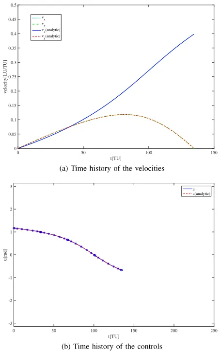
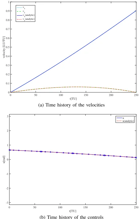
transfer was used as the reference front. Figure 1 shows the cumulative front from all 30 runs, along with 4 representative solutions (marked with crosses) and the analytic solutions with the same ascent time of the representative solutions (marked with circles). The crosses and circles are perfectly overlapping. The trajectories and time histories of the controls and velocities for the 4 representative solutions are plotted in figures 2 and 3 to 6 along with the single objective numerical solution and the analytic solution for the same ascent times. The solution obtained with the proposed approach is very close to both the numerical single objective and the analytic solutions. The discontinuities in the control laws are due to the discretisation scheme and to tolerance on the optimality of the solutions.
B. Maximum Energy Orbit Rise
The original maximum energy orbit rise formulation and some solution strategies can be found in [14] and [6]. In this case, a spacecraft is orbiting around a celestial body, and it is required to increase its total energy by changing its altitude and velocity. The only control variable is again the thrusting angle, and the only other force affecting the spacecraft is gravity (in this case it is considered variable with altitude). The multi-objective extension, proposed in this paper, maximises the final energy and minimises the manoeuvre time:
min
tf,u
J1=tf, J2=−
vr2(tf) +v2t(tf)
2 +
1
r(tf)
!
x[LU]
-20 0 20 40 60 80 100 120
y[LU]
-2 0 2 4 6 8 10 12
[image:6.612.322.549.47.408.2]Trajectory 1 Trajectory 2 Trajectory 3 Trajectory 4
Fig. 2. Trajectories corresponding to the 4 selected points on the Pareto front
t[TU]
0 20 40 60 80 100 120
velocity[LU/TU]
0 0.02 0.04 0.06 0.08 0.1 0.12 0.14 0.16 0.18 0.2
vx vy vx(analytic) vy(analytic)
(a) Time history for the velocities
t[TU]
0 50 100 150 200 250
u[rad]
-3 -2 -1 0 1 2
3 u
u(analytic)
[image:6.612.64.289.48.214.2](b) Time history for the controls
Fig. 3. Time history for velocities and controls, point 1 on the Pareto front
subject to the dynamic constraints:
˙
r =vr
˙
vr =
v2
t
r −
1
r2 +acosu
˙
θ =vt
r
˙
vt =−
vtvr
r +asinu
(20)
t[TU]
0 50 100 150
velocity[LU/TU]
0 0.05 0.1 0.15 0.2 0.25 0.3 0.35 0.4 0.45 0.5
vx vy vx(analytic) vy(analytic)
(a) Time history of the velocities
t[TU]
0 50 100 150 200 250
u[rad]
-3 -2 -1 0 1 2
3 u
u(analytic)
(b) Time history of the controls
Fig. 4. Time history of velocities and controls, point 2 on the Pareto front
whererandθ are the polar coordinates of the spacecraft, vr
and vt are the radial and transversal velocities, and a is the
magnitude of the control acceleration. In this work,a= 1e−2. The boundary conditions are:
r(0) = 1.1; vr(0) = 0
θ(0) = 0; vt(0) =
1 √
1.1
(21)
Following [6], the time domain was subdivided into 30 ele-ments of order 1 for each state and control variable. Control angles were bound between −π and π, while total mission
[image:6.612.61.285.242.599.2]t[TU]
0 20 40 60 80 100 120 140 160 180 200
velocity [LU/TU]
0 0.1 0.2 0.3 0.4 0.5 0.6 0.7
vx vy v
x(analytic)
vy(analytic)
(a) Time history of the velocities
t[TU]
0 50 100 150 200 250
u[rad]
-3 -2 -1 0 1 2
3 u
u(analytic)
[image:7.612.63.286.47.407.2](b) Time history of the controls
Fig. 5. Time history of velocities and controls, point 3 on the Pareto front
VI. CONCLUSION
The paper proposed a novel memetic approach for the solution of multi-objective optimal control problems called MACSoc. The results on two standard optimal control prob-lems with known control laws demonstrated that MACSoc can reliably converge to the Pareto front with good accuracy, good spreading of the solutions and a relatively low number of function evaluations. Further work is required to improve the treatment of infeasible solutions. The simple rejection mechanism is effective in the cases treated in this paper but can prevent progression towards the Pareto front in more complex problems with more difficult constraints.
ACKNOWLEDGMENT
The first author gratefully acknowledges the support of the ESA NPI grant ref. TEC-ECN-SoW-20140806 and of Airbus Defence and Space.
REFERENCES
[1] V. Coverstone-Carroll, J. W. Hartmann and W. J Mason, Optimal multi-objective low-thrust spacecraft trajectories, Computer methods in
applied mechanics and engineering, volume 186, number 2, 2000, pp 387–402
t[TU]
0 50 100 150 200 250
velocity [LU/TU]
0 0.1 0.2 0.3 0.4 0.5 0.6 0.7 0.8 0.9 1
vx vy vx(analytic) vy(analytic)
(a) Time history of the velocities
t[TU]
0 50 100 150 200 250
u[rad]
-3 -2 -1 0 1 2
3 u
u(analytic)
[image:7.612.321.549.49.406.2](b) Time history of the controls
Fig. 6. Time history of velocities and controls, point 4 on the Pareto front
tf[TU]
20 30 40 50 60 70 80
J2
[LU
2/TU 2]
-0.1 -0.05 0 0.05 0.1 0.15 0.2 0.25 0.3
1
2
3
4
Fig. 7. Non dominated solutions of 30 different runs for the maximum energy rise problem. Crosses indicate four representative solutions along the Pareto front.
[2] S. Ober-Blobaum, M. Ringkamp and G. zum Felde,Solving multi-objective optimal control problems in space mission design using discrete mechanics and reference point techniques, IEEE 51st Annual
Conference on Decision and Control (CDC), 2012, pp 5711–5716 [3] C..cn Kaya, H. Maurer, A Numerical Method for Nonconvex
Multi-objective Optimal Control Problems, Computational Optimization and
[image:7.612.327.551.436.596.2]x[LU]
-12 -10 -8 -6 -4 -2 0 2
y[LU]
-4 -3 -2 -1 0 1 2 3 4 5 6
[image:8.612.325.551.45.210.2]Trajectory 1 Trajectory 2 Trajectory 3 Trajectory 4
Fig. 8. Trajectories corresponding to the 4 selected points on the Pareto front
t[TU]
0 10 20 30 40 50 60 70 80
u[rad]
0 0.5 1 1.5 2 2.5 3
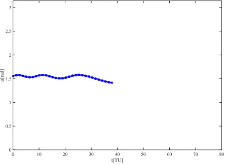
Fig. 9. Time history of the control angle for point 1 on the Pareto front
t[TU]
0 10 20 30 40 50 60 70 80
u[rad]
[image:8.612.64.290.47.219.2]0 0.5 1 1.5 2 2.5 3
Fig. 10. Time history of the control angle point 2 on the Pareto front
[4] J. A. Englander, M. A. Vavrina, A. R. Ghosh,Hybrid Optimal Control for Multiple-Flyby Low-Thrust Mission Design. AAS 15-227, 25th
AAS/AIAA Space Flight Mechanics Meeting, Williamsburg, VA. [5] Zuiani F. and Vasile M., Multi Agent Collaborative Search Based
on Tchebycheff Decomposition, Computational Optimization and
Ap-plications September 2013, Volume 56, Issue 1, pp 189-208, DOI 10.1007/s10589-013-9552-9.
t[TU]
0 10 20 30 40 50 60 70 80
u[rad]
[image:8.612.325.550.242.404.2]0 0.5 1 1.5 2 2.5 3
Fig. 11. Time history of the control angle for point 3 on the Pareto front
t[TU]
0 10 20 30 40 50 60 70 80
u[rad]
[image:8.612.63.288.252.415.2]0 0.5 1 1.5 2 2.5 3
Fig. 12. Time history of the control angle for point 4 on the Pareto front
[6] M. Vasile,Finite elements in time: a direct transcription method for optimal control problems, AIAA 2010-8275, AIAA/AAS Astrodynamics
Specialist Conference, 2 - 5 August 2010, Toronto, Ontario Canada [7] M. Vasile and A. E. Finzi, Direct lunar descent optimisation by
finite elements in time approach, International Journal of Mechanics
and Control, volume 1, number 1, 2000.
[8] H. D. Hodges and R. R. Bless, Weak Hamiltonian finite element method for optimal control problems, Journal of Guidance, Control, and
Dynamics, volume 14, number 1, 1991, pp 148–156.
[9] C. L. Bottasso and A. Ragazzi, Finite element and Runge-Kutta methods for boundary-value and optimal control problems, Journal of
Guidance, Control, and Dynamics, volume 23, number 4, 2000, pp 749– 751.
[10] M. Vasile and F. Bernelli-Zazzera,Optimizing low-thrust and gravity assist manoeuvres to design interplanetary trajectories, The Journal of
the astronautical sciences, volume 51, number 1, 2003, pp 13–35. [11] M. Vasile and F. Bernelli-Zazzera,Targeting a heliocentric orbit
com-bining low-thrust propulsion and gravity assist manoeuvres, Operational
Research in Space & Air, volume 79, 2003.
[12] L. A. Ricciardi and M. Vasile,Improved archiving and search strategies for Multi Agent Collaborative Search, Eurogen 2015
[13] A. E. Bryson, Y. Ho,Applied optimal control: optimization, estimation and control, Revised printing, CRC Press, 1975.
[14] A. L. Herman and B. A. Conway,Direct optimization using collocation based on high-order Gauss-Lobatto quadrature rules, Journal of
[image:8.612.64.287.449.612.2]