Tail risk in pension funds: An analysis using ARCH models and bilinear processes

City, University of London Institutional Repository

Citation

:

Owadally, I. (2014). Tail risk in pension funds: An analysis using ARCH models

and bilinear processes. Review of Quantitative Finance and Accounting, 43(2), pp. 301-331.

doi: 10.1007/s11156-013-0373-9

This is the accepted version of the paper.

This version of the publication may differ from the final published

version.

Permanent repository link: http://openaccess.city.ac.uk/14277/

Link to published version

:

http://dx.doi.org/10.1007/s11156-013-0373-9

Copyright and reuse:

City Research Online aims to make research

outputs of City, University of London available to a wider audience.

Copyright and Moral Rights remain with the author(s) and/or copyright

holders. URLs from City Research Online may be freely distributed and

linked to.

City Research Online: http://openaccess.city.ac.uk/ [email protected]

(will be inserted by the editor)

Tail Risk in Pension Funds: an Analysis using ARCH Models and

Bilinear Processes

Iqbal Owadally

Received: date / Accepted: date

Abstract Pension funding rules and practice contain implicit smoothing and counter-cyclical

mech-anisms. We set up a stylized model to investigate whether this may give rise to tail risk, in the form

of large but rare losses, when pension liabilities are imperfectly but optimally hedged by pension

fund assets. We find that pension losses follow a nonlinear dynamic process, and we derive a complete

description of the stochastic properties of this process using Markov chain and bilinear stochastic

process theory. The resulting pension dynamics resembles that of a modified ARCH model, which

suggests that bursts in volatility may occur, and tail risk may be present. Simulations confirm that

pension losses exhibit skewness, leptokurtosis and heavy tails, specially when cash flow smoothing is

pronounced. Regulators and investors should be aware of the total amount of smoothing in pension

funds as this may contribute to extreme losses, which may adversely affect the security of employee

benefits as well as the valuation of firms with corporate pension plans.

Keywords Pensions·Risk·Heavy-tailed distribution·LARCH process

JEL G23· G28· G32

I. Owadally

Cass Business School, City University London, 106 Bunhill Row, London EC1Y 8TZ, United Kingdom

Tel.: +44-20-70408478

Fax: +44-20-70408572

E-mail: [email protected]

1 Introduction

Risk management in pension plans, as in other financial institutions, requires a careful assessment

of tail risk. Tail risk is the occurrence of extreme losses with a higher probability than may be

normally expected. In the 2008 financial crisis, a large number of pension funds around the world

reported severe difficulties with falling asset values and increasing liabilities.1 _{Large losses occurred,}

and higher contributions were then required from pension plan sponsors. Regulators and legislators

worldwide responded by easing the funding requirements on sponsors. The purpose of this paper

is to investigate the presence of tail risk in corporate pension plans resulting from pension funding

practice and the application of funding rules.

We consider ‘defined benefit’ pension funds. In 2011, such funds had assets totaling $6.6 trillion

in the U.S. and $14.8 trillion globally.2 _{In this paper, we set up a stylized model to investigate the}

mechanism by which extreme losses might arise. Our starting point is that pension liabilities are

not completely marketable and therefore not fully hedgeable. Losses arise from imperfect, albeit

optimal, hedging. However, pension funding rules and practice seek to smooth these cash flows

inter-temporally and counter-cyclically. This delays the emergence of possible funding problems, which

may then accumulate with adverse dynamic effects.

We show in our stylized model that pension losses follow a nonlinear dynamic process, which

we analyze using Markov chain theory and the theory of bilinear stochastic processes. The resulting

pension dynamics resembles that of a modified GARCH process. We therefore posit that the pension

1 _{Global pension funds experienced losses of about 25% of their asset value, as a percentage of pension liability,}

in 2008 (Towers Watson 2011).

2 _{Data from Towers Watson (2011). In ‘defined benefit’ pension plans, employees receive pensions at retirement}

fund loss distribution exhibits leptokurtosis as well as similar extremal behavior to GARCH, and we

investigate this further through stochastic simulations using data on U.S. pension fund returns. Our

key finding is that tail risk—transpiring in the form of a leptokurtic distribution of pension losses

as well as Pareto-like slow decay in the tail of this distribution—is present when pension cash flows

are deferred and smoothed.

An important policy implication is that, as with pension accounting rules, pension funding rules

should be carefully designed to limit the extent of smoothing that is permissible, taking into

ac-count normal corporate practice regarding the management of cash flows, operating leverage and

tax liability. In particular, pension fund managers and regulators should be aware that smoothed

funding methods must be monitored as they may generate risk that may not be observable in normal

financial circumstances, but may manifest itself in the form of rare but large losses. Our research

also informs the policy debate in the European Union concerning the application of the Solvency II

capital adequacy standard to pension funds.

This article is organized along the following lines. The background and motivation for our

re-search, as well as related papers in the literature, are discussed in section 2. A pension fund model

is developed in section 3 and its stochastic properties (strict and weak stationarity, existence of

mo-ments) are investigated in section 4. An analogy with ARCH-type models is also made, which leads us

to the presumption that tail risk may exist in pension losses. Simulations are carried out in section 5

demonstrating tail risk, and we conclude the paper in section 6 with some policy recommendations.

2 Background and Related Literature

2.1 Pension accounting

This research coincides with recent developments in the institutional setting of corporate pension

plans, in terms of accounting, funding, as well as regulatory response to the 2008 financial crisis.

The first key development is in pension accounting. There is a significant literature on the value

relevance of pension accounting information, and also on smoothing in pension expense (as opposed

to pension funding). Jiang (2011) shows that the corridor amortization mechanism used in income

statements under Financial Accounting Standard 158—hereafter FAS 158, see FASB (2006)—is

in-effective and introduces biases leading to overestimation of plan sponsors’ earnings in the long term.

FAS 158 took effect in late 2006. It amends and updates previous accounting rules, notably Financial

Accounting Standard 87—hereafter FAS 87, see FASB (1985)—which incorporated smoothing and

deferred recognition of pension gains and losses on both the balance sheet and income statement.

Mitra and Hossain (2009) examine the implication for valuation of transition adjustments in

ac-counts when FAS 158 was initiated and full recognition of gains and losses was required, rather than

disclosure in footnotes. They find that investors react, and stock prices fall, when the adjustment is

significant, thereby showing that markets do process pension accounting information on the balance

sheet. Both Jiang (2011) and Mitra and Hossain (2009) conclude that the elimination of FAS 87-style

smoothing from the FAS 158 balance sheet is beneficial to investors. On the other hand, Hann et al.

(2007) find that non-smoothed fair-value accounting does not improve, and may impair, the value

relevance of balance sheet and income statements, as compared to smoothed pension accounting

under FAS 87. They suggest that the amortization mechanism of FAS 87 separates more persistent

income from highly volatile gains and losses, thereby helping investors assess value.

Earlier accounting research, based on the older accounting standard FAS 87, shows that investors

fail to price corporate pension liability efficiently (Franzoni and Mar´ın 2006), with firms exploiting the

latitude in assumption-setting and smoothing mechanisms embedded in FAS 87 to manage earnings

(Picconi 2006; Bergstresser et al. 2006). In particular, Franzoni and Mar´ın (2006) show that firms

with significantly underfunded pension plans are overvalued by investors. They suggest that there are

two reasons for this, one being related to accounting (the amortization corridor for pension expenses)

and the other being related to funding. Specifically, mandatory pension contributions—required by

law to enable pension plans to recover to full funding—are spread out over time and impact earnings

2.2 Pension funding

The second key development for corporate pension plans in the U.S. has been in the area of

pen-sion funding. Penpen-sion funding contributions differ from penpen-sion accounting expense, in general. First,

there are mandatory contributions imposed by regulators for minimum funding purposes. U.S.

legisla-tion changed in 2006 with the introduclegisla-tion of the Pension Proteclegisla-tion Act 2006 (hereafter PPA 2006),

which accelerates the remediation of deficits. Broadly, firms had 30 years to fund 90% of liability

before PPA 2006, but now have 7 years to fund 100% of liability. Secondly, there are voluntary or

discretionary contributions, made by pension plan sponsors, which are tax-deductible up to certain

limits. PPA 2006 permits contributions that are deductible up to 150% of the pension liability, a

larger amount than before, therefore encouraging firms to over-fund their pension plans. See

Fran-zoni (2009), Campbell, Dhaliwal and Schwartz (2010, 2012) and Shivdasani and Stefanescu (2010)

for details.

Research in the area of pension funding hinges around the interdependence between sponsors’

financial policy and the investment and funding policies of their pension plans. Rauh (2006) finds

a significant negative association between a firm’s mandatory pension contributions and its capital

investment. Required contributions to underfunded pension plans appear to force companies to divert

cash away from investment. Pension funding rules and practice are therefore critical to the investors in

the firm. Indeed, Franzoni (2009) demonstrates that increased mandatory pension contributions are

followed by depressed stock returns. Campbell, Dhaliwal and Schwartz (2012) find that financially

constrained firms facing an increase in mandatory contributions also face an increase in cost of

capital. In an event study surrounding the date of the introduction of PPA 2006, when minimum

funding rules were tightened, Campbell, Dhaliwal and Schwartz (2010) observe a fall in the stock

market valuation of sponsors with large unfunded pension liabilities and capital expenditures.

PPA 2006 also increased the level of voluntary contributions qualifying for tax-deductibility.

Accordingly, Campbell, Dhaliwal and Schwartz (2010) examine the data to see whether the equity

valuation of corporate sponsors with higher marginal tax rates responds to the adoption of the

rules matter to investors not just because of mandatory contributions but also because of their

effect on discretionary contributions. Shivdasani and Stefanescu (2010) establish that the existence

of a pension fund affects the capital structure of firms and their total amount of financial leverage,

particularly because discretionary pension contributions are a source of tax savings. On the other

hand, Petersen (1994) considers operating leverage, but also concludes that greater flexibility in

pension contributions enables a firm to lower its operating leverage, which may add value in the

presence of market imperfections.

2.3 Financial crisis and counter-cyclical measures

The third key event which has had an impact on pension funds has been the financial crisis in 2008

and the subsequent recession. Pension plan assets worldwide fell by about 25%, as a percentage

of pension liability, in 2008 (Towers Watson 2011). Firms that were financially distressed in the

subsequent recession could not meet funding rules. In the U.S., new legislation was passed in 2008 and

2010 to ease the statutory funding requirements introduced only in 2006 in the Pension Protection

Act (Love, Smith and Wilcox 2011; Yermo and Severinson 2010). The Organization for Economic

Cooperation and Development (OECD) also studied the response of regulators in Europe, Canada

and Japan to the financial crisis: regulators relaxed the exigencies of minimum funding rules, allowing

cash-constrained plan sponsors to bring their plans back to full funding over longer recovery periods,

and partly suspending strict market valuations of pension liabilities in some countries (Yermo and

Severinson 2010).

The OECD has since promulgated counter-cyclical measures and issued guidelines for OECD

member countries which state that “Funding rules should aim to be counter-cyclical, providing

in-centives for the build-up of reserves against market downturns” (OECD 2007). Yermo and Severinson

(2010) are particularly critical of funding rules which compel sponsors to ramp up contributions at

a time when they may be cash-constrained. Such funding rules have systemic pro-cyclical effects in

that they require numerous pension funds to sell assets at the same time to limit deficits, thereby

rules can have second-order macroeconomic effects in that large numbers of firms may curtail

busi-ness investment to fund pension deficits, as documented by Rauh (2006), which slows down economic

recovery and worsens business conditions for firms.

Counter-cyclical measures are also a key part of the Solvency II regime (EIOPA 2012) for

in-surance regulation in the European Union (E.U.). Proposals to apply this regime to pension funds

are under consideration. Solvency II comprises explicit counter-cyclical measures. For example, a

counter-cyclical or liquidity risk premium is used with the effect that capital requirements are

tem-porarily reduced in times of financial crisis. An ‘equity dampener’ adjustment weakens the stress

test on the equity portion of a portfolio when large market falls occur. Large market falls are defined

relative to an averaged value of equity prices.

To some extent, counter-cyclicality is built into pension funding. For example, the U.S. Pension

Protection Act 2006 permits both asset values and liability discount rates (based on the corporate

bond yield curve or at least three different maturity segments) to be averaged over up to 24 months

(OECD 2007). Likewise, Japanese pension liabilities are also discounted using an average of 10-year

bond yields over the previous 5 years, while suitable swap rates are used in the Netherlands with

smoothing permitted for contribution calculation (Yermo and Severinson 2010). In other countries,

counter-cyclical funding may be made explicit through a separate contingency reserve. For example,

Norwegian tax authorities allow payments into a “premium fund”, over and above the payment of

regular premiums, and Swiss pension funds are allowed “asset fluctuation reserves” and “employer

contribution reserves” with typical amortization periods of 5–7 years (OECD 2007). Indeed,

virtu-ally all major economies afford a recovery or amortization period of between 3 to 7 years to their

pension funds to make up funding deficiencies, these periods having been extended temporarily in

the aftermath of the 2008 financial crisis. This is analyzed by Broeders and Chen (2010) who model

pension fund insolvency using Parisian options and use stochastic simulations to investigate the

op-timal recovery period which regulators should allow in order to maximize employees’ utility. They

suggest recovery periods of between 1 and 5 years depending on pension plan features and other

2.4 Other related literature

We briefly mention three other strands of research which are tangential to ours. First, in the

sub-sequent analysis, we exploit some novel results from the econometrics literature on a variant of the

GARCH model called LARCH (Linear-ARCH). This model is extensively studied by Giraitis et al.

(2000, 2004) with further advances by Kristensen (2009) which link LARCH to stochastic bilinear

processes (Pham 1993).

Second, pension insurance is an important aspect of pension funding but is not directly analyzed

here. In the U.S., firms with a defined benefit pension plan pay a premium to the Pension Benefit

Guarantee Corporation (PBGC) which then takes over pension promises (subject to a cap) if a plan

sponsor becomes bankrupt. There is a flat premium per participant plus an additional premium

dependent on the unfunded pension liability, but the premium is not risk-based. This creates a put

option for plan sponsors which encourages a more aggressive pension fund investment policy. See,

for example, Rauh (2009), Love, Smith and Wilcox (2011) and McGill et al (2004, p. 801) for further

details.

Third, the issue of optimal pension funding and investment is not addressed in this paper. The

lit-erature on this subject (see e.g. Berkelaar and Kouwenberg 2003; Rudolf and Ziemba 2004; Owadally

and Haberman 2004a; Josa-Fombellida and Rinc´on-Zapatero 2006) employs broad utility and

ob-jective functions on measures of fund levels and contributions, and does not focus on tail risk. This

indicates that optimal funding solutions may need to be re-assessed in the light of our findings.

Blake (2006b, p. 83–91) summarizes the issues affecting pension investment policy, including tax and

pension insurance effects.

3 Pension Fund Model

3.1 Pension liabilities

A corporate pension fund consists of the assets held against the pension liabilities of a firm. First,

ageEand leave the plan at retirement ageR(whereE, R∈N_{andR > E), whereupon they receive}

a retirement benefit which consists of a life annuity. (For example,E = 27 andR= 67.) No other

benefit is payable.

We also assume that there is no demographic or longevity risk and that survival proceeds exactly

according to a life table{ℓx}, whereℓxis the number of individuals alive at agex∈ {E, E+ 1, . . .}.

The survival probability from agexto ageyis thereforeℓy/ℓx(Dickson et al. 2009, p. 42). The age

profile of the pension plan population is stable.

A suitable spot rate curve, which may be used to discount and value pension liabilities, is assumed

to exist.3 Denote the (τ −t)-year continuously compounded spot rate at timet ass(t, τ). That is,

s(t, τ) is the yield-to-maturity at timetof a zero-coupon bond maturing at timeτ. The present value

at timetof a deferred life annuity paying $1 yearly in advance from retirement ageRtill death for

an individual agedx≤Rat timetis

α(t, x) =

∞

X

j=0

exp (−(R−x+j)s(t, t+R−x+j)) ℓR+j/ℓx. (1)

An annuity is purchased at retirement at which point an individual leaves the plan. The actual

pension or annuity income received every year in retirement is usually a function of the number of

years of service and the projected pensionable salary of the individual. The pensionable salary could

be the final salary of the individual or his career-average salary. See for example Sundaresan and

Zapatero (1997), McGill et al (2004, p. 235), Blake (2006b, p. 194), and Dickson et al. (2009, p.

306–312) for more details.

We assume that salary proceeds according to a deterministic age-based scale (Dickson et al. 2009,

p. 292). Since the age profile of the plan membership is stable, payroll is constant. The pension benefit

accrues to a plan member as he works and contributions are made to the plan. We may therefore

define a benefit accrual functionmxwheremxis the benefit that has accrued to an individual agedx

3 _{This is typically based on the yields on high-quality corporate bonds to reflect the credit risk present in pension}

(whereE≤x≤R). From retirement ageRuntil death, an individual receives a pension or annuity

income of mR every year. We assume that, at entry into the plan at age E, an employee is not

immediately endowed with benefit rights, so thatmE = 0. The accrued liability for an individual

agedx(wherex≤R) at timetmay therefore be valued asmxα(t, x).

While individuals are working and are members of the plan, their employer contributes to the

pension fund, which accumulates and then pays out for the annuity when they retire. How much

to contribute during the working lifetime is the subject of various actuarial cost methods. These

provide a systematic way of accumulating funds to provide retirement benefits. Associated with

these methods are different measures of the pension liability. A straightforward discussion of these

measures is given by Novy-Marx and Rauh (2011) with more details given by McGill et al (2004, p.

617).

We assume that the pension liability is measured using the Projected Benefit Obligation (PBO).

Under the PBO, mx is a function of the projected salary at retirement of an individual aged x.

For accounting purposes in the U.S., pension liability is reported using the PBO under FAS 158.

For funding purposes, the U.S. Pension Protection Act 2006 requires underfunding to be measured

using a metric for which the PBO is a very close proxy (Shivdasani and Stefanescu 2010; Campbell,

Dhaliwal and Schwartz 2010).4

The pension liability is denoted by Yt. When measured as the PBO, it is the sum of accrued

liabilities for every individual in the plan. There areℓx members agedx (whereE≤x≤R), so

Yt = R

X

x=E

mxℓxα(t, x). (2)

To simplify the liability dynamics, we shall assume that the spot rate curve{s(t, τ), τ = 1,2, . . .}

is subject to small, parallel shifts only. Associated with the spot rate curve at time t is a single,

4 _{The PBO is also the preferred measure of pension liability under several international accounting standards. An}

alternative measure of pension liability is the Accumulated Benefit Obligation (ABO) which is defined in FAS 87. It is also used by pension funding regulators in various countries because it is a termination measure, as compared with the PBO which is a broader, going-concern measure (Broeders and Chen 2010). Our subsequent analysis holds for the ABO rather than the PBO, as long asmxis re-defined as a function of the current salary of an individual,

term-independent discount rateδtat which we can discount the liability cash flows to obtainYtas

in equation (2). We may regardδtas the yield-to-maturity or internal rate of return, at timet, on a

notional dedicated bond portfolio whose cash flows match the pension liability cash flows as closely

as possible.

We assume that the spot rate curve is subject to stochastic shocks such that it mean-reverts to

a long-run curve {bs(τ), τ = 1,2, . . .}, corresponding to which we have a single, term-independent

discount rate δ. We may therefore viewδ as approximately equal to the average yield-to-maturity

on the aforementioned notional bond portfolio. Further, defineY to be the liability calculated using

{sb(τ)}, or equivalently usingδ. Shocks to the term structure translate into shocks to δt (centered

approximately aroundδ), and consequently into shocks toYt(centered approximately aroundY).

Finally, we denote by DY the volatility or modified duration of the pension liability when

dis-counted at rateδ. That is, DY = −Y−1∂Y /∂δ. We may then employ a first-order approximation

centered aroundδ.

Assumption 1 The spot rate curve {s(t, τ), τ = 1,2, . . .} is subject to small, shape-preserving

stochastic perturbations. The dynamics of the pension liabilityYt is approximately given by

Yt = Yt−1exp (−DY(δt−δt−1)). (3)

3.2 Normal pension cash flows

Actual pension fund cash flows may differ from reported cash flows, in general. In particular,

contri-butions may be different from pension accounting expense. We separate the pension cash flows into

a normal cash flow, denoted by Zt, and a supplementary cash flow. The latter is required to make

up shortfalls in the fund or to reduce contributions in the event of surpluses, and is defined later in

section 3.4. The normal cash flow Zt is further decomposed into three cash flows. The first is the

benefit paid out from the pension fund at time t. This is Zt(1)= mRℓRα(t, R), since there are ℓR

The second cash flow is the required contribution under the actuarial cost method to be paid

at timet. For a plan member aged x (whereE ≤x < R), this is equal to the present value of the

benefit that the member will accrue during the following year, that is (mx+1−mx)α(t, x). The total

required contribution paid into the fund at timetis obtained by summing over all workers, noting

again that there areℓx workers agedx.

Zt(2) = R_X−1

x=E

(mx+1−mx)ℓxα(t, x). (4)

Zt(2) is equivalent to the service cost in the calculation of pension expense in FAS 158 and its

predecessor FAS 87.

The final component of normal cash flowZtis an additional interest charge on the liability, given

byZt(3)=e −δ_(δ

t−δ)Yt. The termδtYtcorresponds to the interest cost in FAS 158 pension expense

(and FAS 87), and is a finance charge on the liability (Blake 2006a, p. 62). This term is discounted

here because of the modeling assumption that cash flows occur at the start of the year. The termδYt

is analogous to the expected return on plan assets in FAS 158 (and FAS 87). This is a negative item

in that a positive expected return reduces pension cost (Grant et al. 2007; McGill et al 2004, p. 729).

We consider an economic valuation of liabilities, without the FAS 158 objective of pension expense

smoothing, and plan assets are assumed to closely hedge liabilities (see Assumption 2 below), so no

long-term expected rate of return assumption is required here.

The normal cash outgo from the fund at timetis thereforeZt=Zt(1)−Z

(2)

t +Z

(3)

t . Further cash

flows may be required to pay off prior-service cost representing benefit enhancements attributable to

plan members’ past service or benefit rights obtained at the inception of the plan (Grant et al. 2007;

McGill et al 2004, pp. 729–731). However, these are one-off, amortized payments and are ignored

here.

We show in Appendix A that the normal cash outgo is approximately a constant percentage of

the liability.

Zt/Yt ≈ 1−e−δ. (5)

Equation (5) holds approximately because of the simplified liability dynamics of Assumption 1

equa-tion (5) follows from the earlier assumpequa-tion of a stable age profile. The benefit payout and liability

vary stochastically only with interest rates. In practice, they will also depend on other stochastic

variables such as inflation, mortality, employee turnover etc.

Since Zt−1 ≈Yt−1(1−e−δ) from equation (5), we may re-write the liability dynamics in equa-tion (3) as

Yt = (Yt−1−Zt−1) exp

rLt

. (6)

In the above, rL

t = δ −DY(δt−δt−1) and may be described as the ‘liability return’, this term being borrowed from the one-period models of Leibowitz and Henrikssan (1988) and Sharpe and

Tint (1990), and their multi-period extension by Rudolf and Ziemba (2004).

3.3 Pension fund assets

We now turn to the pension fund assets. In the light of equation (5), it is natural to express the assets

as a proportion of liabilities. The funding status (difference between liabilities and assets, scaled by

liabilities) or funded ratio (ratio of plan assets to liabilities) are key quantities and are arguably more

important than the PBO or fair value of plan assets by themselves: see for example Rauh (2009),

Franzoni (2009) and Rudolf and Ziemba (2004).

We denote byFtthe market value of pension fund assets at timetas a percentage of liabilityYt.

It is also convenient to defineFt= 1−Ft as the unfunded liability at timet as a percentage ofYt.

The unfunded liability represents the deficit in the fund. We also defineCt to be a supplementary

contribution, again as a percentage of liabilityYt, paid into the fund. The cash flowCtis additional

to the normal cash flow and is paid to reduce any deficit. In the case of a surplus,Ctmay be negative

so that the overall contribution is reduced.

The budget constraint on the pension fund is FtYt = (Ft−1Yt−1−Zt−1+Ct−1Yt−1) exp rAt

,

in dollar terms, whererAt is the stochastic return on pension fund assets in time interval (t−1, t).

With the help of equations (5) and (6) we may rewrite the budget constraint as

Ft = (Ft−1+Ct−1−Z) exp

rAt −r L t +δ

Since rAt is the asset return andrLt is the liability return, the term rtA−rtL may be described as

a continuously compounded ‘surplus return’ (Leibowitz and Henrikssan 1988; Rudolf and Ziemba

2004). This brings us to a discussion of the relationship between the pension fund assets and pension

liabilities.

In general, a perfect hedge for pension liabilities cannot be synthetized because these liability

cash flows are not marketable. Some pension fund risk is therefore unhedgeable, at least partially.

For example, credit risk, related to insolvency of the firm sponsoring the pension fund, may be

hedged through credit default swaps, but these may be unavailable in the required volume or may

be substituted for credit spread risk (Blake 2006b, pp. 269–271). The pension fund may also be

restricted by regulation from taking excessive long, short or complex derivative positions in the

securities issued by the firm to avoid agency conflicts and to encourage diversification. The very

long duration of pension liabilities and scarcity of long-duration securities create duration mismatch;

pension liabilities cannot be perfectly immunized despite the use of derivatives overlays (Adams and

Smith 2009).

Background unhedgeable risks may also be present, chief among which is wage inflation risk

(Berkelaar and Kouwenberg 2003; Blake 2006b, p. 268). Because retirees want to maintain their

living standard in retirement, pensions are a function of salary before retirement. The market in

inflation-indexed securities and inflation swaps may not be deep enough for all pension funds to

hedge inflation risk, and basis risk will remain as local wages deviate from consumer prices. A more

subtle background risk, which is difficult to hedge, is covenant risk. This pertains to the strength of

the sponsor’s commitment to the plan and the risk that the sponsor decides to terminate the plan

or freeze new accrual.5

5 _{The Pensions Act 2004 in the United Kingdom requires explicit consideration of the strength of the sponsor}

Returning to the surplus returnrAt −rLt, we assume that a perfect hedge is not possible, because

of market incompleteness as discussed above. The pension fund manager pursues an imperfect but

optimal hedge instead, which entails a noisy replication or hedging error.6

Assumption 2 The stochastic surplus returnrA

t −rLt satisfiesE

exp rA t −rtL

= 1 and

{rAt −rLt, t∈Z}is a sequence of independent and identically distributed (i.i.d.) random variables.

Note that we make no assumption about specific probability distributions in Assumption 2.

3.4 Supplementary pension cash flows

We discussed the normal pension fund cash flow (denoted byZt) in section 3.2. The total cash flow

from the plan sponsor to the pension fund may differ fromZtand we refer to this variation as a

sup-plementary cash flow or supplmentary contribution (denoted byCt). Supplementary cash flows may

occur because of mandatory contributions imposed by regulators, under the U.S. Pension Protection

Act 2006 (PPA 2006), for example. They may also occur because of voluntary contributions to take

advantage of the tax-deductibility of pension contributions, or to maximize operational leverage. See

the discussion in section 2.2 and references therein.

We propose to model the supplementary cash flowCtin a generic way as follows. First, we define

the pension fund loss as the unexpected change in pension fund assets relative to pension liabilities.

Lt = E[Ft| Ft−1] − Ft, (8)

whereFtis information available at timet. (A gain is merely a negative loss.)

6 _{In theory, this may be achieved using a quadratic (variance-minimizing) hedge or an entropy-minimizing hedge}

Assumption 3 The supplementary cash flowCtthat is paid by the plan sponsor into the pension

fund at timetis given by

Ct = π′Lt. (9)

In the above,π= (π1, . . . , πp)′ satisfyingPp_j=1e−(j−1)δπj = 1, and Lt= (Lt, Lt−1, . . . , Lt−p+1)′, wherep∈N_.

The motivation behind Assumption 3 is that supplementary cash flows tend to be retrospective

in nature. In equation (9), Ct depends on present and past losses contained in the loss vector Lt.

For example, mandatory contributions are a function of the unfunded liability in the pension plan,

and therefore on the history of losses. The choice of funding parameter vector πin equation (9) is flexible enough to capture the complex intertwining of funding and fiscal rules, and firms’ incentives

to contribute to their pension funds. Thus, an economic downturn may lead to pension losses in

years which coincide with sponsor distress, leading to a reduced funding contribution (within

min-imum funding rules). In subsequent years, however, plan sponsors may increase contributions for

tax or operational reasons when their balance sheets recover. See the discussion in section 2.2, and

particularly Rauh (2006), Shivdasani and Stefanescu (2010) and Petersen (1994).

Assumption 3 also reflects the counter-cyclical measures and cash flow-smoothing behavior

de-scribed in section 2.3. Smoothing in liability discount rates and asset values—as permitted in the

U.S. under the Pension Protection Act 2006 (PPA 2006) and as detailed in Actuarial Standards

of Practice Nos. 4, 27 and 44 (see ASB 2007a,b, 2009)—leads to a funding position that implies a

smoothed average of market values. The condition in Assumption 9 that the funding parameters or

filter weights{πj}satisfyPpj=1e

−(j−1)δ_π

j = 1 signifies that losses are fully paid off. Note that this

is a generalized setting which encapsulates amortization over p years ifπj (for j = 1, . . . , p) is set

equal to the reciprocal of the present value of ap-year annuity-due. In this case, we envisage that the

dimensionpof the loss vector equals the maximum recovery period (for example,p= 7 years under

PPA 2006). However, p might be greater than the typical amortization period if funding practice

Proposition 1 The lossLtsatisfies the stochastic recurrence relation

Lt = εt β′Lt−1−1

, (10)

whereεt= exp(rAt −rtL)−1andβ= (β1, . . . , βp)′, whereβj=ejδ−Pjk=1e

(j−k+1)δ_π

kforj∈[1, p].

The proof of Proposition 1 is given in Appendix B. Proposition 1 exhibits the dynamics of pension

losses{Lt}as a function of the sequence of asset-liability hedging or mismatch errors{εt}. If pension

liabilities were liable to perfect hedging, thenεt= 0∀tand no pension loss would occur.

4 Bilinear Processes and ARCH Models

4.1 Stochastic properties

In order to make further progress with our analysis of the pension fund, we need to consider the

probabilistic properties of{Lt}in equation (10). In this section, we find the conditions under which

{Lt, Ft, Ct} is ergodic, strictly stationary, weakly stationary and has finite moments.

It is helpful to rewrite the stochastic process{Lt, t∈Z}in equation (10) as follows:

Lt = εtvt, (11a)

vt = p

X

j=1

βjLt−j − 1. (11b)

We assume throughout that the initial conditions on equation (10), or equation set (11), consist of

known finite valuesLl, . . . ,Ll−p+1 for some timel <0 in the distant past.

4.2 Weak stationarity and first two moments

Some elementary results about{Lt}may be obtained in a straightforward way and we collect them

in the following proposition. Under Assumption 2,{εt, t∈Z}is a sequence of i.i.d. random variables

withE_{εt= 0. Note that, by construction in equation (10) and under Assumption 2,εtis independent}

Proposition 2

(i) {Lt} is a martingale difference sequence,ELt= 0and Cov [Lt, Lτ] = 0fort6=τ.

(ii) Assume thatE_ε2_t=σ2_{<∞. If and only ifσ}2_β′_{β<1, then{L}

t}is weakly stationary and

VarLt = σ2

.

1−σ2β′β

. (12)

The proof of Proposition 2 is straightforward and is relegated to Appendix C. The asset-liability

hedge works ‘on average’, since the hedging error satisfies E_{εt =} E_exp(rtA_−rL_{t)−1 = 0 under}

Assumption 2. Part (i) of Proposition 2 thus shows that the pension loss is zero on average. Part (ii)

shows that the filterπ(or equivalentlyβ) in the funding contribution calculation under Assumption 3 must be carefully chosen to satisfyσ2β′β<1 if one wishes to avoid a pension loss with an infinite variance. The poorer the hedge is, the more stringent this condition becomes. In other words, if the

hedging or replication error volatilityσ is larger, the choice of funding parameterπ(or equivalently

β) is more restricted.

4.3 State-space representation

The loss process{Lt}in equation (10) can be written in state-space form as follows.

Lt+1 = At+1Lt + Bt+1, (13a)

Lt = CtLt + Dt. (13b)

In the state equation (13a), the coefficient matrixAt is a p×p companion matrix which, in block

form, is given by

At =

   

ξεt βpεt

Ip−10p−1   

, (14)

where ξ = (β1, . . . , βp−1),Ip−1 is the (p−1)×(p−1) identity matrix, and0p−1 is a (p−1)×1 column vector of zeros.Btis ap×1 row vector,

The observation equation (13b) is trivial, with Ct= (1,0, . . . ,0) andDt= 0 (a scalar). Note that

{At} and{Bt}are sequences of i.i.d. matrices and vectors respectively.

Equation (13a) is in the form of a first-order vector stochastic difference equation. Assuming the

initial conditions stated for equation (11),Ll→0p asl→ −∞, and equation (13a) is solved by

Lt = ∞

X

j=0

At· · ·At−jBt−j−1 + Bt. (16)

A theorem from Bougerol and Picard (1992a) states the conditions for strict stationarity of

generalized autoregressive processes, such as {Lt} in equation (16), in terms of the top Lyapunov

exponent,

γ = lim

t→∞

1

t E[logkAt· · ·A1k]. (17)

Theorem 1 (Bougerol and Picard 1992a) Suppose that{Lt} is irreducible and that

E_log+_kAtk<∞and E_log+_{kBtk<∞. Then{Lt} is strictly stationary if and only ifγ <0.}

The notation log+(x) = max(0,logx) is used in the above. The requirement that γ < 0 in

Theorem 1 is analogous to the requirement that the discount factor be less than one for the present

value of a non-random perpetuity to be finite.

4.4 Bilinear processes

In order to apply Theorem 1, we must elucidate whether the pension fund losses, expressed as{Lt},

form an irreducible Markov chain. A bilinear representation is helpful in this regard, and also gives

us access to conditions for the existence of moments.

Definition 1 (Bilinear process) (Pham 1993)The process{xt, t∈Z}is a bilinear process if it

satisfies

xt = q1

X

j=1

ajxt−j + q2

X

j=0

cjǫt−j + q3

X

j=1

q4

X

k=1

bjkxt−jǫt−k (18)

The descriptor ‘bilinear’ refers to the fact that equation (18) is linear in {xt} and, separately,

linear in {ǫt}, but not linear in both because of the product term xt−jǫt−k. Pham (1985, 1986,

1993) shows that a specific class of bilinear process, for whichbjk = 0 for j < k, can be written in

state-space form with the coefficient matrices of the state equation being polynomials in the noise

ǫt, these polynomials being of order 2 at most. Denote the coefficient matrices in the relevant state

equation byAet and Bet, whereAet is the leading coefficient. The following theorem gives a simple

condition for strict stationarity with finite second moments.

Theorem 2 (Pham 1985)Suppose thatE_ǫ4_{t <∞. The bilinear process{xt}in equation (18), with}

bjk= 0forj < k, is strictly stationary with finite second moments if and only if the matrix equation

Q = E

h e

AtQAe′t

i

+ VarBet (19)

admits a positive solution inQ.

Pham (1986, 1993) also establishes a sufficient condition for the existence of even moments in

the bilinear process {xt}, in terms of the spectral radius (denoted byρ) of the expectation of the

Kronecker product of the leading coefficient matrix with itselfntimes (denoted by⊗nin superscript).

Theorem 3 (Pham 1986, 1993) If E_ǫ2_tm _{< ∞ and ρ}

E h

e

A⊗2m t

i

< 1, where m ∈ N_{, then}

E_x2_tm_<∞.

Returning to Theorem 1, we must address the issue of irreducibility before being able to apply

Theorem 1. Kristensen (2009, Theorem 5) considers this issue for a somewhat different class of

bilinear processes to which he refers as Class 2:

yt = a0 +

q1

X

j=1

ajyt−j + q3

X

j=1

bjjyt−jǫt−j. (20)

An irreducible Markov chain is never reduced, in terms of its transitions, to a strict subset of its

state space: it can ‘travel’ to any point of its state space given enough time. If the Markov chain is

viewed as a deterministic system with its noise process being a sequence of decision variables, then

(2009) thus considers the controllability of the bilinear process{yt}in equation (20) in terms of the

polynomials

Φ(z) = 1−

q1

X

j=1

ajzj, Θ(z) = q3

X

j=1

bjjzj−1, (21)

formed from the coefficients in equation (20). The noise process, viewed as a control variable, must

also be unconstrained and Kristensen (2009) shows that it must be absolutely continuous.

Theorem 4 (Kristensen 2009)The Markov chain in the state-space representation of the bilinear

process{yt}in equation (20)is irreducible if and only if (i)ǫthas an absolutely continuous component

(wrt. Lebesgue measure) in the neighborhood of zero, and (ii) the polynomials Φ(z) and Θ(z)have

non-coincident zeros.

4.5 Stochastic properties of the pension fund

We state the conditions for strict stationarity, ergodicity and the existence of even moments of the

pension fund process {Lt, Ft, Ct} in the following proposition, which we prove by reference to the

theorems cited above. We also derive the first two moments explicitly.

Proposition 3 (i) Suppose that εt has an absolutely continuous component in a neighborhood of

zero. A necessary and sufficient condition for{Lt} in equation(10)to be strictly stationary and

ergodic is thatγ <0, whereγ is defined in equation (17)withAt defined in equation (14).

(ii) Assume thatE_ε2_{t =σ}2 _{<∞. Thenσ}2β′_β

<1 is a necessary and sufficient condition for{Lt}

to be strictly stationary with finite second moments.

(iii) IfE_ε2_tm_{<∞and ρ} E_A⊗2m t

<1, wherem∈N_{, then}E_L2_tm_<∞.

(iv) Stationary first and second moments (provided they exist) are as follows:

(a) E_Lt=E_Ft=E_{Ct= 0and}E_{Ft= 1.}

(b) Cov [Lt, Lτ] = 0fort6=τ.

(c) Q:= VarLt=σ2/(1−σ2β′β).

(e) If 0≤τ ≤p−1, thenCov [Ct, Ct−τ] =QPpj=1−τ(ππ

′

)(j,j+τ)

andCov [Ft, Ft−τ] =QPp_j=1−τ(λλ′)(j,j+τ).

Ifτ ≥p, thenCov [Ct, Ct−τ] = Cov [Ft, Ft−τ] = 0.

The proof of Proposition 3 is given in Appendix D. Propositions 2 and 3 supply a complete

description of the conditions required on the asset-liability hedging errors{εt} and on the funding

parameter vector π (or equivalently β and λ) to achieve stationarity and finite moments in the pension fund process.

4.6 ARCH-type models and tail risk

In this section, we draw an analogy between the pension loss process {Lt} in equation (10) and

ARCH-type models. This tells us about the behavior of the tail of the distribution of the pension loss.

Heavy tails signify that extreme unfavorable losses occur more frequently than expected compared

to the normal distribution, and suggest that there is significant tail risk in the pension fund.

Definition 2 (GARCH) (Bollerslev 1986)The GARCH(q2, q1) process{zt, t∈Z}satisfies

zt = σtǫt, σt2 = a0 +

q2

X

k=1

dkσt2−k + q1

X

j=1

cjz2t−j, (22)

wherea0∈R++,cj, dk∈R+, andǫtis as in Definition 1.

The link between GARCH models and vector stochastic difference equations and Markov chain

theory is well-known. It is exploited by Bougerol and Picard (1992b) and, latterly, by Kristensen

(2009) to derive conditions for strict stationarity and ergodicity of GARCH processes. The link

between GARCH and bilinear processes is less well-known but is noted by Tong (1990, pp. 116, 136).

Rewriting equation (22) as

σt2 = a0 +

q2

X

k=1

dkσt2−k + q1

X

j=1

cjσt2−jǫ2t−j (23)

and comparing the above to equation (18) or (20) makes the point that the GARCH squared-volatility

σ2

Indeed, both GARCH and bilinear models were developed with the aim of capturing non-constant

volatility. Simulated data from both GARCH and bilinear models show that: (i) sample paths make

large excursions from the mean, (ii) their distributions exhibit leptokurtosis, and (iii) QQ-plots

indicate heavy-tailedness. See Fan and Yao (2003, pp. 153, 183) for example. This suggests that the

pension loss process{Lt} of equation (10) may also exhibit heavy tails.

A recent variant of the GARCH process is the LARCH (Linear-ARCH) which is extensively

studied by Giraitis et al. (2000, 2004).

Definition 3 (LARCH) (Giraitis et al. 2000) The process {wt, t∈Z}is a LARCH process if

it satisfies

wt = σtǫt, σt = a0 +

∞

X

j=1

cjwt−j, (24)

wherea0, cj∈Rwitha06= 0, andǫtis as in Definition 1.

In the LARCH process in equation (24), volatility is a linear combination of past values of the

process. Contrast this with the standard GARCH process in equation (22), wheresquared volatility

is a linear combination of pastsquared values of the process.

The LARCH process describes two stylized facts of asset return data that are not adequately

reflected by the standard GARCH model (Fan and Yao 2003, p. 170): (i) long memory or long-range

dependence, and (ii) the leverage effect. The former describes the empirical observation of profound

autocorrelation in absolute and squared returns, along with very slow decay as lag increases, slower

than the exponential decay implied by GARCH. The latter describes the higher increase in volatility

that is experienced after a fall in the market, as compared with volatility increases after a rise in

market values, and as contrasted with the symmetric behavior of volatility in GARCH.

Now, {Lt} in equation (11) and the LARCH process {wt} in equation (24) differ only in the

finiteness of the series. Proposition 3 appears to suggest that the conditions on parameters of the

loss process become progressively more stringent as one transits from requiring strict stationarity,

to weak stationarity, to the existence of moments of increasing order, until one reaches a sufficiently

of the LARCH ‘volatility’ term σt in equation (24), and they use the combinatorial formalism of

diagrams to find various moments of wt and σt. They also find that the existence of higher-order

moments requires progressively greater restriction on the LARCH parameters.

Now, a well-known moment inequality in probability theory suggests that infinite higher-order

moments should lead to a heavy-tailed probability distribution. At a fundamental level, heavy tails

can be explained by an application of renewal theory to stochastic difference equations, resulting in

products of random matrices, as shown in section 4.3 (Kesten 1973). This is suggestive, therefore, of

possible significant tail risk in the pension fund. If large losses occur with a higher probability than

anticipated, then larger contributions will be required from plan sponsors. As argued by Franzoni

and Mar´ın (2006), this may be underestimated by investors who therefore overprice firms with

significantly underfunded pension plans.

5 Stochastic Simulations

In this section, we use stochastic simulations of the model in section 3 to complement the analysis

of section 4 and investigate tail risk in the pension fund.

Tail risk We investigate the distribution of both the unfunded liability Ft and the cash flow or

supplementary contribution Ct. In the case of Ft, we are considering the risk that the pension

fund does not accumulate enough assets. Leibowitz and Henrikssan (1988) and Sharpe and Tint

(1990) refer to this as surplus risk. In the case ofCt, we are considering the risk that capital must be

unexpectedly diverted to the pension fund to make up for large losses or deficits. This can potentially

result in bankruptcy of the corporate plan sponsor (credit risk) or closure of the plan (covenant risk).

We are interested in the extremes of bothFt andCt, and therefore in tail risk.

Simulation inputs Some representative parameter values and assumptions are required to simulate

the pension fund. To draw meaningful, realistic conclusions, we allow for liability growth through

inflation. We assume that real returns are i.i.d., consistent with Assumption 2. We use the OECD

between 1988 and 2005 and we fit a normal distribution, with mean 6.83% and standard deviation

8.91%, to the log-return. Note that this is return per annum and net of price inflation.

Initialization and normalization There is no evidence in the OECD data (Tapia 2008) that the

surveyed pension funds are managed solely with a view to hedging liabilities, but we assume that

this is the case, again consistent with Assumption 2. More precisely, we assume that pension assets

hedge inflation in pension liabilities. Hence, we setδ= 6.83% and εt∼i.i.d. lognormal with a zero

mean and a standard deviation of 9.6%.7 The pension liability Y is normalized at 100% and an

initial normal contribution of 4.2% is calculated.

Averaging and amortization To operationalize the counter-cyclical and smoothing behavior of

pen-sion funds, we simulate the U.S. practice of averaging asset values and amortizing resultant losses.

The averaging period is denoted bynand the amortization period bym, so that the orderp of the

loss process{Lt}in equation (10) is p=m+n−1. Details are provided in Appendix E.

Simulation outputs The loss Lt and unfunded liability Ft are expressed as a percentage of the

liability, whereas the supplementary contributionCtis expressed as a percentage of the normal

con-tribution. Simulations are performed for different smoothing levels, that is, for different combinations

of amortization periodmand averaging periodn.

Computation To capture the tail of the distributions, we carry out 100,000 simulations, with checks

for convergence using 50,000 and 200,000 simulations. We use a fixed seed to generate reproducible

pseudo-random numbers and minimize sampling error when comparing results. To investigate strict

stationarity, we estimate the top Lyapunov exponent, as defined in equation (17), using (see Bougerol

and Picard 1992a)

γ a.s.= lim

t→∞

1

t logkAt· · ·A1k. (25)

7 _{If logX∼N(µ, σ}2_{), then VarX=e}2µ+σ2

eσ2

Fig. 1 Plots of smoothing parametersnversusmshowing frontiers of strict stationarity (A), weak stationarity (B), existence of 4th moments (C) and existence of 6th moments (D). The region of stationarity or existence of moments is the region under and including the relevant curve.

For weak stationarity, we use the condition in part (ii) of Proposition 2 directly, so no simulation

is required. To investigate the existence of moments, we could use the condition in part (iii) of

Proposition 3 but this is a sufficient condition and could be unnecessarily restrictive, so we use

stochastic simulation instead to test whether moments are finite.

Stationarity and existence of moments Our results are presented in Figure 1, which shows regions

of stationarity or existence of moments, that is, the maximum values of n for different values of

m for which stationarity or existence of moments holds.8 As expected from the discussion in

sec-tion 4.6, more stringent condisec-tions, in the form of shorter averaging and amortizasec-tion periods, apply

as moments of a higher order are required to exist. This is indicative of a heavy-tailed distribution.

8 _{Equivalently, the frontiers in Figure 1 give the maximummfor variousn. Note thatm, n∈}N_{, so a polynomial}

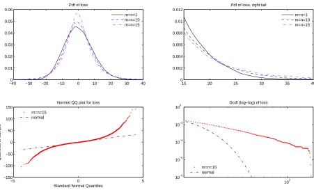
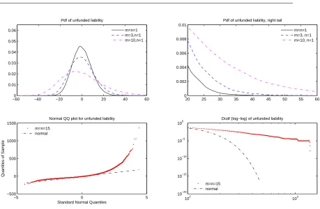
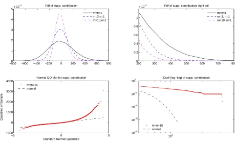
Probability plots Non-parametric estimates of the probability density functions (pdf) and the

decu-mulative distribution functions (dcdf), as well as normal quantile-quantile (QQ) plots for the loss,

the unfunded liability and the supplementary contribution are shown in Figures 2, 3 and 4

respec-tively. (The dcdf is the complementary cdf, i.e. 1−cdf.) Since we are concerned with tail risk, the

behaviour of the right tail is of interest. The QQ-plots, in the bottom left panels of Figures 2, 3 and

4, show deviation from normality in the right tails.Lt,FtandCtall exhibit heavy-tailedness on the

right.

Heavy-tailedness A measure of heavy-tailedness is the tail index introduced by Kesten (1973). This

captures the fact that heavy-tailed distributions have tails that are Pareto-like and that decay like

a power law. The tail indexκis an estimate of the rate of tail decay in the probability distribution

of a random variableX (Fan and Yao 2003, p. 156):

P_{(X > x) ∼ Cx}−κ_{, (26)}

whereC is some constant and∼means that the ratio of the l.h.s. and r.h.s. of equation (26) tends

to 1 in the limit asx → ∞. The log-log plots of the dcdf’s of Lt,Ft and Ct, in the bottom right

panels of Figures 2, 3 and 4 respectively, exhibit linearity. This gives a strong indication that their

tails decay slowly according to a power law. In our numerical investigations, the power law decay was

particularly evident for large smoothing parameter values (that is, largemandn). For comparison,

we also show the tails of the normal distribution, with corresponding mean and standard deviation,

which exhibit fast decay.

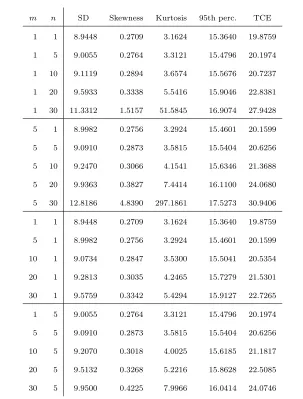
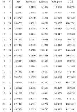
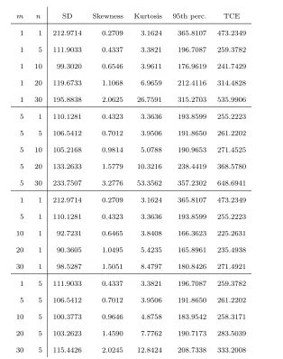
Tabulated statistics Various statistics for the loss, unfunded liability and supplementary contribution

are shown in Tables 1, 2 and 3 respectively. There is some minor repetition in the Tables, e.g. statistics

form=n= 5, but this ensures legibility and aids with interpretation.

First moments First moment values are within±0.5%, consistent with zero expectation from part (iv)

−400 −30 −20 −10 0 10 20 30 40 0.01 0.02 0.03 0.04 0.05 0.06

Pdf of loss

m=n=1 m=n=10 m=n=15

15 20 25 30 35 40

0 0.002 0.004 0.006 0.008 0.01 0.012

Pdf of loss, right tail

m=n=1 m=n=10 m=n=15

−5 0 5

−150 −100 −50 0 50 100 150

Standard Normal Quantiles

Quantiles of Sample

Normal QQ plot for loss

m=n=15 normal 102 10−8 10−6 10−4 10−2 100

Dcdf (log−log) of loss

m=n=15 normal

Fig. 2 Probability density estimates for the lossLt (top left), with right tail enlarged (top right), for different

smoothing parametersmand n. The normal QQ-plot (bottom left) shows deviation from normality in the tails. The log-log plot of the decumulative distribution function (bottom right) shows the slowly decaying Pareto-like right tail of the distribution of the loss, compared to the normal distribution.

Third and fourth moments We observe from Tables 1–3 that the loss, unfunded liability and

sup-plementary contribution are all positively skewed and leptokurtic, with both skewness and kurtosis

increasing as smoothing increases (i.e. as either m or n increases). It is noteworthy that the pdf

curves of the loss in Figure 2 cross twice on either side of the mean, but this happens only once for

the pdf curves of the unfunded liability in Figure 3.

Risk measures We investigate three risk measures: (i) The standard deviation is a classical measure

of risk for symmetrically distributed random variables, and is used in Markowitz mean-variance

portfolio theory, for example. (ii) The 95th percentile is commonly used, usually appearing in the

−600 −40 −20 0 20 40 60 0.01 0.02 0.03 0.04 0.05 0.06

Pdf of unfunded liability

m=n=1 m=3,n=1 m=10,n=1

20 25 30 35 40 45 50 55 60 0 0.002 0.004 0.006 0.008 0.01

Pdf of unfunded liability, right tail

m=n=1 m=3, n=1 m=10, n=1

−5 0 5

−500 0 500 1000 1500

Standard Normal Quantiles

Quantiles of Sample

Normal QQ plot for unfunded liability

m=n=15 normal

102 103

10−20 10−15 10−10 10−5 100

Dcdf (log−log) of unfunded liability

m=n=15 normal

Fig. 3 Probability density estimates for the unfunded liabilityFt (top left), with right tail enlarged (top right),

for different smoothing parametersmandn. The normal QQ-plot (bottom left) shows deviation from normality in the right tail. The log-log plot of the decumulative distribution function (bottom right) shows the slowly decaying Pareto-like right tail of the distribution of the unfunded liability, compared to the normal distribution.

a continuously distributed random variableX with cdfFX(x), the 95th percentile isFX−1(0.95) and

the TCE isE_{X |X > F}−1

X (0.95)

.

Risk of underfunding (Ft) In Tables 1 and 2, the loss and unfunded liability exhibit monotonically

increasing standard deviations, 95th percentiles and tail conditional expectations as either mor n

increases. The risk of underfunding therefore increases as smoothing increases. This is reasonable

because more smoothing means that losses are paid off more slowly, so that losses tend to accumulate,

leading to more volatile pension fund deficits.

Cash flow risk (Ct) Whereas funding risk increases with more smoothing, cash flow risk behaves in

−8000 −600 −400 −200 0 200 400 600 800 1

2 3 4 5x 10

−3 _{Pdf of supp. contribution}

m=n=1 m=3,n=1 m=10,n=1

200 300 400 500 600 700 800 0 0.2 0.4 0.6 0.8 1

x 10−3 Pdf of supp. contribution, right tail

m=n=1 m=3, n=1 m=10, n=1

−5 0 5

−1000 0 1000 2000 3000 4000

Standard Normal Quantiles

Quantiles of Sample

Normal QQ plot for supp. contribution

m=n=15 normal 103 10−20 10−15 10−10 10−5 100

Dcdf (log−log) of supp. contribution

m=n=15 normal

Fig. 4 Probability density estimates for the supplementary contribution Ct (top left), with right tail enlarged

(top right), for different smoothing parametersmandn. The normal QQ-plot (bottom left) shows deviation from normality in the right tail. The log-log plot of the decumulative distribution function (bottom right) shows the slowly decaying Pareto-like right tail of the distribution of the supplementary contribution, compared to the normal distribution.

1. Low smoothing levels.Risk inCtappears to have a minimum wrt.mandn, at least for low values

ofmandn. In Table 3, the standard deviation and the 95th percentile decrease and then increase

asnincreases when m= 1, 5 (and also asmincreases whenn= 1, 5). The behavior of the tail

conditional expectation is somewhat more ambiguous but also appears to have a minimum. This

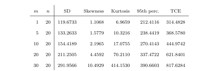
feature of a minimum in contribution risk is also reproduced in Table 4 when m = n and m

increases.

2. High smoothing levels.For larger values ofn(resp.m), risk inCtbehaves as inLtandFtin that

it increases monotonically asm(resp.n) increases. We show only the case forn= 20 in Table 5

m n SD Skewness Kurtosis 95th perc. TCE 1 1 8.9448 0.2709 3.1624 15.3640 19.8759 1 5 9.0055 0.2764 3.3121 15.4796 20.1974 1 10 9.1119 0.2894 3.6574 15.5676 20.7237 1 20 9.5933 0.3338 5.5416 15.9046 22.8381 1 30 11.3312 1.5157 51.5845 16.9074 27.9428

5 1 8.9982 0.2756 3.2924 15.4601 20.1599 5 5 9.0910 0.2873 3.5815 15.5404 20.6256 5 10 9.2470 0.3066 4.1541 15.6346 21.3688 5 20 9.9363 0.3827 7.4414 16.1100 24.0680 5 30 12.8186 4.8390 297.1861 17.5273 30.9406

1 1 8.9448 0.2709 3.1624 15.3640 19.8759 5 1 8.9982 0.2756 3.2924 15.4601 20.1599 10 1 9.0734 0.2847 3.5300 15.5041 20.5354 20 1 9.2813 0.3035 4.2465 15.7279 21.5301 30 1 9.5759 0.3342 5.4294 15.9127 22.7265 1 5 9.0055 0.2764 3.3121 15.4796 20.1974 5 5 9.0910 0.2873 3.5815 15.5404 20.6256 10 5 9.2070 0.3018 4.0025 15.6185 21.1817 20 5 9.5132 0.3268 5.2216 15.8628 22.5085 30 5 9.9500 0.4225 7.9966 16.0414 24.0746

Table 1 Standard deviation, skewness, kurtosis, 95th percentile and tail conditional expectation of the lossLtfor

various combinations ofm,n.

The above observations about contribution risk are consistent with the results of Owadally and

Haberman (1999, 2004a) in the context of optimal pension funding. These authors use a simple

pension fund model and look only at standard deviation rather than tail risk. Their explanation,

in terms of a controlled process, is nevertheless applicable here. Smoothing, at low levels, means

that the recognition of random losses is deferred so that contributions are dampened. But too much

smoothing leads to feedback with long delays: losses are paid off too slowly and they accumulate

m n SD Skewness Kurtosis 95th perc. TCE

1 1 8.9448 0.2709 3.1624 15.3640 19.8759

1 5 14.3627 0.4995 3.4593 25.4955 33.7607 1 10 21.3724 0.7939 4.1891 38.9556 53.4606 1 20 39.6760 1.5662 8.6251 73.5585 110.1710 1 30 75.9424 3.4658 44.9189 129.4896 223.7662

5 1 13.8046 0.4784 3.4204 24.4489 32.2817 5 5 20.1227 0.7461 4.0338 36.5750 49.8702 5 10 27.7233 1.0638 5.1931 51.2338 72.7586 5 20 48.9183 2.0575 13.8148 89.5563 140.4511 5 30 97.8561 5.1100 108.4428 154.5248 286.5379

1 1 8.9448 0.2709 3.1624 15.3640 19.8759

5 1 13.8046 0.4784 3.4204 24.4489 32.2817 10 1 19.1937 0.7167 3.9599 34.8725 47.2743 20 1 29.0291 1.1599 5.6909 53.9020 77.1303 30 1 38.6314 1.6503 9.1320 71.6141 108.1702 1 5 14.3627 0.4995 3.4593 25.4955 33.7607 5 5 20.1227 0.7461 4.0338 36.5750 49.8702 10 5 25.9875 1.0047 4.9242 47.8631 67.5400 20 5 37.1329 1.5634 8.2782 69.4890 103.4388 30 5 48.7451 2.2625 15.6745 89.3260 142.1886

Table 2 Standard deviation, skewness, kurtosis, 95th percentile and tail conditional expectation of the unfunded

liabilityFt for various combinations ofm,n.

pension fund. Thus, the application of counter-cyclical and smoothed funding rules, which aim to

reduce contribution volatility for pension plan sponsors, may have a counter-productive effect if they

are not properly calibrated.

6 Conclusion

Like other financial institutions, corporate pension funds suffered deep losses in the financial crisis

m n SD Skewness Kurtosis 95th perc. TCE 1 1 212.9714 0.2709 3.1624 365.8107 473.2349 1 5 111.9033 0.4337 3.3821 196.7087 259.3782 1 10 99.3020 0.6546 3.9611 176.9619 241.7429 1 20 119.6733 1.1068 6.9659 212.4116 314.4828 1 30 195.8838 2.0625 26.7591 315.2703 535.9906

5 1 110.1281 0.4323 3.3636 193.8599 255.2223 5 5 106.5412 0.7012 3.9506 191.8650 261.2202 5 10 105.2168 0.9814 5.0788 190.9653 271.4525 5 20 133.2633 1.5779 10.3216 238.4419 368.5780 5 30 233.7507 3.2776 53.3562 357.2302 648.6941

1 1 212.9714 0.2709 3.1624 365.8107 473.2349 5 1 110.1281 0.4323 3.3636 193.8599 255.2223 10 1 92.7231 0.6465 3.8408 166.3623 225.2631 20 1 90.3605 1.0495 5.4235 165.8961 235.4938 30 1 98.5287 1.5051 8.4797 180.8426 271.4921 1 5 111.9033 0.4337 3.3821 196.7087 259.3782 5 5 106.5412 0.7012 3.9506 191.8650 261.2202 10 5 100.3773 0.9646 4.8758 183.9542 258.3171 20 5 103.2623 1.4590 7.7762 190.7173 283.5039 30 5 115.4426 2.0245 12.8424 208.7338 333.2008

Table 3 Standard deviation, skewness, kurtosis, 95th percentile and tail conditional expectation of the

supple-mentary contributionCtfor various combinations ofm,n.

m n SD Skewness Kurtosis 95th perc. TCE

1 1 212.9714 0.2709 3.1624 365.8107 473.2349 5 5 106.5412 0.7012 3.9506 191.8650 261.2202 10 10 112.6476 1.3109 6.8758 206.8592 303.4156 15 15 142.3291 2.1914 15.5769 254.3503 412.1991 20 20 211.2505 4.4592 70.2110 337.4722 621.8401

Table 4 Standard deviation, skewness, kurtosis, 95th percentile and tail conditional expectation of the

m n SD Skewness Kurtosis 95th perc. TCE 1 20 119.6733 1.1068 6.9659 212.4116 314.4828 5 20 133.2633 1.5779 10.3216 238.4419 368.5780 10 20 154.4189 2.1965 17.0755 270.4143 444.9742 20 20 211.2505 4.4592 70.2110 337.4722 621.8401 30 20 291.9566 10.4929 414.1530 390.6603 817.6284

Table 5 Standard deviation, skewness, kurtosis, 95th percentile and tail conditional expectation of the

supple-mentary contributionCtfor variousmwhenn= 20.

funding and accounting rules, which permit cash flows and costs to be spread over time. In this

paper, we sought to establish whether the smoothing mechanisms entrenched in pension funding

rules and practice could be related to large pension losses and deficits.

We reviewed the evidence in the accounting literature that spreading cash flows over time hinders

investors’ efficient valuation of firms. There is also significant evidence in the corporate finance

liter-ature that increases in mandatory pension contributions negatively impact firms’ capital investment

and are accompanied by depressed stock returns subsequently. Pension funding rules and practice

also influence the value of firms because of the tax savings and operational leverage that flexibility in

discretionary pension contributions affords, after allowing for market imperfections. The mechanism

underlying funding for pension plans is therefore important to investors and management, as well as

to the employee membership of these plans.

The evidence, from the U.S. and worldwide, that funding rules are implemented in a

counter-cyclical fashion was also reviewed. This was particularly visible in the aftermath of the financial

crisis in 2008. Proposed funding rules in the European Union are explicit in allowing for

counter-cyclical measures. These are also implicit—through averaging in liability discount rates, asset values

and choice of valuation parameters—in funding practices utilized in the U.S. and elsewhere. These

methods are intended to limit the volatility of cash flows required from plan sponsors.

We built a stylized model, with the starting premise that pension liabilities are optimally but