Sensitivity of the advanced LIGO detectors at the beginning of gravitational wave astronomy

Sensitivity of the Advanced LIGO detectors at the beginning of gravitational

wave astronomy

D. V. Martynov,1 E. D. Hall,1 B. P. Abbott,1 R. Abbott,1 T. D. Abbott,2 C. Adams,3 R. X. Adhikari,1 R. A. Anderson,1 S. B. Anderson,1 K. Arai,1 M. A. Arain,4 S. M. Aston,3 L. Austin,1 S. W. Ballmer,5 M. Barbet,4D. Barker,6 B. Barr,7 L. Barsotti,8 J. Bartlett,6M. A. Barton,6I. Bartos,9 J. C. Batch,6 A. S. Bell,7 I. Belopolski,9J. Bergman,6J. Betzwieser,3

G. Billingsley,1 J. Birch,3 S. Biscans,8 C. Biwer,5 E. Black,1 C. D. Blair,10C. Bogan,11R. Bork,1 D. O. Bridges,3 A. F. Brooks,1C. Celerier,12G. Ciani,4F. Clara,6D. Cook,6S. T. Countryman,9M. J. Cowart,3D. C. Coyne,1A. Cumming,7

L. Cunningham,7 M. Damjanic,11R. Dannenberg,1 K. Danzmann,13,11C. F. Da Silva Costa,4 E. J. Daw,14D. DeBra,12 R. T. DeRosa,3R. DeSalvo,15K. L. Dooley,16S. Doravari,3J. C. Driggers,6S. E. Dwyer,6A. Effler,3T. Etzel,1M. Evans,8 T. M. Evans,3M. Factourovich,9H. Fair,5D. Feldbaum,4,3R. P. Fisher,5S. Foley,8M. Frede,11P. Fritschel,8V. V. Frolov,3

P. Fulda,4 M. Fyffe,3 V. Galdi,15J. A. Giaime,2,3K. D. Giardina,3 J. R. Gleason,4 R. Goetz,4S. Gras,8 C. Gray,6 R. J. S. Greenhalgh,17H. Grote,11C. J. Guido,3K. E. Gushwa,1E. K. Gustafson,1R. Gustafson,18G. Hammond,7J. Hanks,6

J. Hanson,3 T. Hardwick,2 G. M. Harry,19 J. Heefner,1,*M. C. Heintze,3 A. W. Heptonstall,1 D. Hoak,20 J. Hough,7 A. Ivanov,1 K. Izumi,6M. Jacobson,1 E. James,1 R. Jones,7 S. Kandhasamy,16 S. Karki,21M. Kasprzack,2 S. Kaufer,13 K. Kawabe,6W. Kells,1N. Kijbunchoo,6E. J. King,22P. J. King,6D. L. Kinzel,3J. S. Kissel,6K. Kokeyama,2W. Z. Korth,1 G. Kuehn,11P. Kwee,8M. Landry,6B. Lantz,12A. Le Roux,3B. M. Levine,6J. B. Lewis,1V. Lhuillier,6N. A. Lockerbie,23 M. Lormand,3M. J. Lubinski,6 A. P. Lundgren,11T. MacDonald,12M. MacInnis,8 D. M. Macleod,2 M. Mageswaran,1 K. Mailand,1S. Márka,9Z. Márka,9A. S. Markosyan,12E. Maros,1I. W. Martin,7R. M. Martin,4J. N. Marx,1K. Mason,8

T. J. Massinger,5 F. Matichard,8 N. Mavalvala,8 R. McCarthy,6 D. E. McClelland,24 S. McCormick,3 G. McIntyre,1 J. McIver,1E. L. Merilh,6M. S. Meyer,3P. M. Meyers,25J. Miller,8R. Mittleman,8G. Moreno,6C. L. Mueller,4G. Mueller,4

A. Mullavey,3J. Munch,22L. K. Nuttall,5 J. Oberling,6 J. O’Dell,17P. Oppermann,11Richard J. Oram,3B. O’Reilly,3 C. Osthelder,1D. J. Ottaway,22H. Overmier,3J. R. Palamos,21H. R. Paris,12W. Parker,3Z. Patrick,12A. Pele,3S. Penn,26

M. Phelps,7 M. Pickenpack,11 V. Pierro,15I. Pinto,15J. Poeld,11M. Principe,15L. Prokhorov,27O. Puncken,11 V. Quetschke,28E. A. Quintero,1F. J. Raab,6H. Radkins,6P. Raffai,29C. R. Ramet,3C. M. Reed,6S. Reid,30D. H. Reitze,1,4

N. A. Robertson,1,7 J. G. Rollins,1 V. J. Roma,21J. H. Romie,3 S. Rowan,7 K. Ryan,6 T. Sadecki,6E. J. Sanchez,1 V. Sandberg,6V. Sannibale,1R. L. Savage,6R. M. S. Schofield,21B. Schultz,11P. Schwinberg,6D. Sellers,3A. Sevigny,6 D. A. Shaddock,24Z. Shao,1B. Shapiro,12P. Shawhan,31D. H. Shoemaker,8D. Sigg,6B. J. J. Slagmolen,24J. R. Smith,32

M. R. Smith,1 N. D. Smith-Lefebvre,1 B. Sorazu,7 A. Staley,9 A. J. Stein,8 A. Stochino,1 K. A. Strain,7R. Taylor,1 M. Thomas,3P. Thomas,6K. A. Thorne,3E. Thrane,33C. I. Torrie,1G. Traylor,3G. Vajente,1G. Valdes,28A. A. van Veggel,7 M. Vargas,3A. Vecchio,34P. J. Veitch,22K. Venkateswara,35T. Vo,5C. Vorvick,6S. J. Waldman,8M. Walker,2R. L. Ward,24 J. Warner,6B. Weaver,6R. Weiss,8T. Welborn,3P. Weßels,11C. Wilkinson,6P. A. Willems,1L. Williams,4B. Willke,13,11

L. Winkelmann,11 C. C. Wipf,1 J. Worden,6 G. Wu,3 H. Yamamoto,1 C. C. Yancey,31H. Yu,8 L. Zhang,1 M. E. Zucker,1,8 and J. Zweizig1

1_{LIGO, California Institute of Technology, Pasadena, California 91125, USA} 2

Louisiana State University, Baton Rouge, Louisiana 70803, USA 3_{LIGO Livingston Observatory, Livingston, Louisiana 70754, USA}

4

University of Florida, Gainesville, Florida 32611, USA 5_{Syracuse University, Syracuse, New York 13244, USA} 6

LIGO Hanford Observatory, Richland, Washington 99352, USA 7_{SUPA, University of Glasgow, Glasgow G12 8QQ, United Kingdom} 8

LIGO, Massachusetts Institute of Technology, Cambridge, Massachusetts 02139, USA 9_{Columbia University, New York, New York 10027, USA}

10

University of Western Australia, Crawley, Western Australia 6009, Australia

11_{Albert-Einstein-Institut, Max-Planck-Institut für Gravitationsphysik, D-30167 Hannover, Germany} 12

Stanford University, Stanford, California 94305, USA 13_{Leibniz Universität Hannover, D-30167 Hannover, Germany} 14

The University of Sheffield, Sheffield S10 2TN, United Kingdom

15_{University of Sannio at Benevento, I-82100 Benevento, Italy and INFN, Sezione di Napoli,}

I-80100 Napoli, Italy

16_{The University of Mississippi, University, Mississippi 38677, USA} 17

Rutherford Appleton Laboratory, HSIC, Chilton, Didcot, Oxon OX11 0QX, United Kingdom 18_{University of Michigan, Ann Arbor, Michigan 48109, USA}

19

American University, Washington, D.C. 20016, USA

20_{University of Massachusetts-Amherst, Amherst, Massachusetts 01003, USA} 21

23_{SUPA, University of Strathclyde, Glasgow G1 1XQ, United Kingdom} 24

Australian National University, Canberra, Australian Capital Territory 0200, Australia 25_{University of Minnesota, Minneapolis, Minnesota 55455, USA}

26

Hobart and William Smith Colleges, Geneva, New York 14456, USA 27_{Faculty of Physics, Lomonosov Moscow State University, Moscow 119991, Russia}

28

The University of Texas Rio Grande Valley, Brownsville, Texas 78520, USA 29_{MTA Eötvös University,“Lendulet”Astrophysics Research Group, Budapest 1117, Hungary}

30

SUPA, University of the West of Scotland, Paisley PA1 2BE, United Kingdom 31_{University of Maryland, College Park, Maryland 20742, USA} 32

California State University Fullerton, Fullerton, California 92831, USA 33_{Monash University, Victoria 3800, Australia}

34

University of Birmingham, Birmingham B15 2TT, United Kingdom 35_{University of Washington, Seattle, Washington 98195, USA}

(Received 5 April 2016; published 2 June 2016)

The Laser Interferometer Gravitational Wave Observatory (LIGO) consists of two widely separated 4 km laser interferometers designed to detect gravitational waves from distant astrophysical sources in the frequency range from 10 Hz to 10 kHz. The first observation run of the Advanced LIGO detectors started in September 2015 and ended in January 2016. A strain sensitivity of better than 10−23=pffiffiffiffiffiffiHz was achieved around 100 Hz. Understanding both the fundamental and the technical noise sources was critical for increasing the astrophysical strain sensitivity. The average distance at which coalescing binary black hole systems with individual masses of 30M_⊙ could be detected above a signal-to-noise ratio (SNR) of 8 was 1.3 Gpc, and the range for binary neutron star inspirals was about 75 Mpc. With respect to the initial detectors, the observable volume of the Universe increased by a factor 69 and 43, respectively. These improvements helped Advanced LIGO to detect the gravitational wave signal from the binary black hole coalescence, known as GW150914.

DOI:10.1103/PhysRevD.93.112004

I. INTRODUCTION

The possibility of using interferometers as gravita-tional wave detectors was first considered in the early 1960s [1]. In the 1970s and 1980s, long-baseline broad-band laser interferometric detectors were proposed with the potential for an astrophysically interesting sensitivity [2,3]. Over several decades, this vision evolved into a worldwide network of ground based interferometers [4–6]. These instruments target gravitational waves produced by compact binary coalescences, supernovae, nonaxisymmetric pulsars and cosmological background in the audio frequency band, from 10 Hz to 10 kHz[7]. The network of widely separated instruments is required to distinguish gravitational wave signals from intrinsic noise transients [8] and to localize astrophysical sources in the sky [9].

The first generation of LIGO detectors consisted of two 4-km-long and one 2-km-long interferometers in the United States [10]: L1 in Livingston, Louisiana, H1 and H2 in Hanford, Washington. They were opera-tional until 2010 and reached their designed strain sensitivity over the detection band, with a peak sensitivity of 2×10−23=pffiffiffiffiffiffiHz at 200 Hz. Astrophysically relevant

results were produced by the initial LIGO detectors [11–14], however, no gravitational wave signals were detected.

The second generation Advanced LIGO detectors [15] were installed in the existing facilities from 2010 to 2014. This new generation of instruments was designed to be 10 times more sensitive than initial LIGO, and promised to increase the volume of the observable universe by a factor of 1000. Commissioning of the newly installed detectors took place from mid 2014 to mid 2015. In September 2015, Advanced LIGO began the era of gravitational wave astronomy with its first observation run (O1), collecting data until January 2016[16]. This run has culminated in the first direct detection of gravitational waves from the black hole coalescence, GW150914 [17,18]. This system con-sisted of two black holes of about 30 solar mass each which merged about 400 Mpc away.

While the detectors were not yet operating at design sensitivity during the first observation run, their astrophysi-cal reach was already significantly greater than that of any previous detector in the frequency range 10 Hz–10 kHz. Around 100 Hz, the strain sensitivity was8×10−24=pffiffiffiffiffiffiHz. For a system consisting of two30M_⊙ black holes the sky location and source orientation-averaged range, for an optimal signal-to-noise ratio (SNR) detection threshold of 8, was 1.3 Gpc, whereas for a binary neutron star

system the range was 70–80 Mpc. This range is≃4.1and ≃3.5times higher than that of the initial LIGO detectors, resulting in a factor of ≃70 and ≃40 improvement, respectively, of the volume that is probed and LIGO’s detection potential.

In this paper we describe the noise characterization of the Advanced LIGO detectors during the first observation run. Section II introduces the optical configuration, control system and calibration of the detectors. SectionIIIanalyzes the performance of the detectors and describes all inves-tigated noise sources. We end with the conclusions in Sec. IV.

II. INTERFEROMETER CONFIGURATION

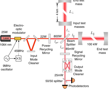
In general relativity, a gravitational wave far away from the source can be approximated as a linear disturbance of the Minkowski metric,g_μν¼ημνþh_μνwith the space-time deformation expressed as a dimensionless strain,h_μν. In a Michelson interferometer we define the differential displacement as L¼L_∥−L_⊥, where L_∥ and L_⊥ are the lengths of the inline arm and the perpendicular arm, respectively, as shown in Fig. 1. With equal macroscopic arm lengths, L₀≃L_∥≃L_⊥, the gravitational wave strain and the differential arm length are related through the simple equationLðfÞ ¼L_∥−L_⊥ ¼hðfÞL₀, wherehis the average differential strain induced into both arms at frequency f.

The test masses are four suspended mirrors that form Fabry-Perot arm cavities. These mirrors can be considered as inertial masses above the pendulum resonance frequency (∼1Hz). Any noise present in the differential arm channel is indistinguishable from a gravitational wave signal. Residual seismic noise, thermal noise associated with the vertical suspension resonance, and the gravity-gradient background limits the useful frequency range to above 10 Hz as discussed in Sec. III A. Motion of the four test masses form the two most relevant degrees of freedom: differential and common arm lengths. While gravitational waves couple to the differential arm length, the common arm length is highly sensitive to changes in the laser frequency according to the equation

L_þðfÞ ¼L∥þL⊥

2 ¼L0

VðfÞ

ν ; ð1Þ

where ν¼2.82×1014 Hz is the laser carrier frequency,

VðfÞ is the laser frequency noise. Signal L_þ is used for frequency stabilization of the main laser as discussed in Sec. III E.

The central part of the interferometer is usually called the dual-recycled Michelson interferometer. Its function is to optimize the detector’s response to gravitational waves. The power recycling cavity, formed by the power recycling mirror and the two input test masses, increases optical power incident on the arm cavities and passively filters

laser noises as discussed in Sec.III E. The signal recycling cavity, formed by the signal recycling mirror and the two input test masses, is used to broaden the response of the detector beyond the linewidth of the arm cavities. The Michelson interferometer, formed by the beam splitter and the two input test masses, is controlled to keep the antisymmetric port near the dark fringe. The dual recycled Michelson interferometer can thus be described by three degrees of freedom: power recycling cavity length lp;þ, signal recycling cavity lengthl_s;þand Michelson lengthl₋, defined as

l_p;þ ¼l_prþl∥þl⊥

2

ls;þ ¼lsrþ

l_∥þl_⊥

2

l₋ ¼l_∥−l_⊥; ð2Þ

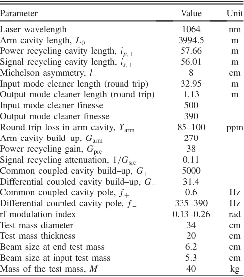
The most important optical parameters of the Advanced LIGO interferometers are summarized in TableI. The beam size here is defined as the distance from the beam center to the point when intensity is reduced by a factor1=e2. The cavity polefpdetermines the width of the cavity resonance and is given by

fp¼

Yc

8πL₀; ð3Þ

wherecis the speed of light andY≪1is the total optical loss in the cavity, including transmission of the input and output cavity couplers as well as scattering and absorption losses. The response of the Advanced LIGO interferom-eters is diminished at high frequencies due to common and differential coupled cavity poles (f_þ andf₋) according to the transfer functions

K_þ ¼ fþ

ifþf_þ; K−¼

f₋

ifþf₋: ð4Þ

Several critical improvements distinguish Advanced LIGO from the initial detectors[15]. The much improved seismic isolation system[22]reduces the impact of ground vibrations. All photodetectors, used in the observing mode, are installed in vacuum to avoid the coupling of ambient acoustic noise to the gravitational wave channel. The larger and heavier test masses lead to a reduction of quantum radiation pressure induced motion and thermal noise[23]. Multistage pendulums with a monolithic lower suspension

stage [24] filter ground motion and improve suspension thermal noise. Furthermore, instead of using coil-magnet actuation pairs to exert control forces on the test masses, electrostatic interaction is employed. This actuation scheme helps to avoid coupling of magnetic noise to the gravita-tional wave channel[25,26].

Lower arm cavity loss, coupled with an increase in the available power from the Nd:YAG laser, allows up to 800 kW of laser power to circulate in the arm cavities— 20 times higher than in initial LIGO—significantly reducing the high frequency quantum noise. The use of optically stable folded recycling cavities allows for better confinement of the spatial eigenmodes of the optical cavities[27]. The signal recycling cavity[28], which was not present in initial LIGO, was introduced at the antisymmetric port to broaden the frequency response of the detector and improve its sensitivity at frequencies below 80 Hz and above 200 Hz. Because O1 was the first observing run, and work remains to be done on the detectors to bring them to their design sensitivity, not all of the interferometer parameters were at their design values during O1. Most notably, the laser power resonating in the arm cavities was 100 kW instead of the planned 800 kW. More power in the arm cavities improves the shot noise level as discussed in Sec. III B. Circulating optical power will be increased in future observational runs. Additionally, the signal recycling mirror transmissivity was 36%, in contrast to the design value of 20%. This higher transmissivity of the signal recycling mirror improves the quantum noise in the frequency range from 60 Hz to 600 Hz at the price of reducing the sensitivity at other frequencies. Finally, the best measured Advanced LIGO sensitivity in the frequency range 20–100 Hz, as discussed in Sec.III, is limited by a wide range of understood technical noise sources as well as currently unknown noise sources.

Figure 2 shows the Advanced LIGO detector’s sensi-tivity during the first observing run. The performance of both the L1 and H1 detectors is compared to the initial LIGO sensitivity and the design sensitivity: the improve-ment with respect to S6 was 3–4 times at 100 Hz and higher frequencies. Below 100 Hz, the upgraded seismic isolation system yielded even larger improvements, with more than an order-of-magnitude-better strain sensitivity for frequen-cies below 60 Hz. The sensitivity of Advanced LIGO can also be quantified as maximum distance at which a given astrophysical source would be detectable, known as“ hori-zon distance.” Figure 3 shows the horizon distance as a function of the chirp mass for coalescence of neutron star (M≲2M_⊙) and black hole (M≳2M_⊙) binaries. For chirp masses≲100M_⊙, the horizon distance increases with chirp mass since the gravitational wave signal is stronger from heavier binary systems. However, the signal also shifts toward lower frequencies (and out of the LIGO frequency band) for massive binary systems, and horizon distance decreases for chirp masses≳100M_⊙.

TABLE I. List of optical parameters.

Parameter Value Unit

Laser wavelength 1064 nm

Arm cavity length,L₀ 3994.5 m Power recycling cavity length,lp;þ 57.66 m Signal recycling cavity length,ls;þ 56.01 m Michelson asymmetry,l₋ 8 cm Input mode cleaner length (round trip) 32.95 m Output mode cleaner length (round trip) 1.13 m Input mode cleaner finesse 500

Output mode cleaner finesse 390

Round trip loss in arm cavity,Yarm 85–100 ppm Arm cavity build–up,Garm 270

Power recycling gain,Gprc 38 Signal recycling attenuation,1=Gsrc 0.11 Common coupled cavity build–up,G_þ 5000 Differential coupled cavity build–up,G₋ 31.4

Common coupled cavity pole,f_þ 0.6 Hz Differential coupled cavity pole,f₋ 335–390 Hz rf modulation index 0.13–0.26 rad

Test mass diameter 34 cm

Test mass thickness 20 cm

A. Interferometer controls

In operation the laser light needs to resonate inside the optical cavities. This requires that the residual longitudinal motion of the optical cavities be kept within a small fraction of the laser wavelength [30]. The suspended mirrors naturally move by ∼1μm in the microseismic band (∼100mHz)—much larger than the width of a resonance. To suppress this motion, a sophisticated length sensing

and control system is employed, using both the well-known Pound-Drever-Hall technique [31,32] and a version of homodyne detection known as “DC readout” [33]. Table II shows linewidths and requirements for residual root-mean-square (RMS) motion of the main interferomet-ric degrees of freedom.

An electro-optic modulator generates radio frequency (rf) phase modulation sidebands at 9 MHz and 45 MHz, symmetrically spaced about the laser carrier frequency. The Pound-Drever-Hall technique is used to sense all longi-tudinal degrees of freedom except for the differential arm channel. Feedback control signals actuate on the suspended mirrors, using either coil-magnet or electrostatic actuation. The common arm cavity length is also used as a reference to stabilize the laser frequency, with sub-mHz residual fluctuations (in detection band).

The gravitational wave signal is extracted at the anti-symmetric port of the interferometer, where fluctuations in the differential arm cavity length are sensed. The arm cavities are held slightly off-resonance by an amount referred to as the differential arm offset ΔL. This offset of roughly 10 pm generates the local oscillator field, which is necessary for the DC readout. An output mode cleaner [34] located between the antisymmetric output and the homodyne readout detectors, is used to filter out the rf sidebands as well as any higher-order optical modes, as these components do not carry information about the differential arm cavity length.

A similar feedback control scheme is employed to keep the optical axes aligned relative to each other and the laser beam centered on the mirrors[35]. This system is required to maximize the optical power in the resonant cavities and keep it stable during data collection. A set of optical wavefront sensors is used to sense internal misalignments [36]. At the same time, DC quadrant photodetectors sense beam positions relative to a global reference frame. The test mass angular motions are stabilized to 3 nrad rms, keeping power fluctuations in the arm cavities smaller than 1% on the time scale of a few hours.

B. Strain calibration

For the astrophysical analyses, the homodyne readout of the differential arm cavity length needs to be calibrated into dimensionless units of strain[37]. This is complicated by FIG. 2. The strain sensitivity for the LIGO Livingston detector

(L1) and the LIGO Hanford detector (H1) during O1. Also shown is the noise level for the Advanced LIGO design (gray curve) and the sensitivity during the final data collection run (S6) of the initial detectors.

100 101 102 103 101

102 103 104 105

Advanced LIGO design Advanced LIGO, H1 (2015) Enhanced LIGO (2010)

FIG. 3. The sensitivity to coalescing compact binaries for the Advanced LIGO design, first observation run (O1) and the final run with the initial detectors (S6). The traces show the horizon distance, which is the distance along the most sensitive direction of the interferometer for a binary inspiral system that is seen head-on and for a signal-to-noise ratio of 8. The horizontal axis is the chirp mass which is defined as M¼ ð1þzÞμ35M25, where M¼M₁þM₂ is the total mass, μ¼M₁M₂=M is the reduced mass, and z is the cosmological redshift. Units are in solar masses, M_⊙. The horizon distance is computed for the case of equal masses M₁¼M₂ and using the inspiral–merger model from[29].

TABLE II. The linewidths of Pound-Drever-Hall signals and the requirements for residual RMS motion for the main inter-ferometric degrees of freedom.

Degree of freedom Linewidth Residual

the fact that the feedback servo for this degree-of-freedom has a bandwidth of about 100 Hz, extending well into the band of interest. Denoting the control signal sent to the end test masses withs, and the error signal, as measured by the photodiodes in units of W, with e, the strain signalhis

h¼AsþC−1e; ð5Þ

whereAis the calibration of the actuator strength into strain and is computed using dynamical models. The transfer functionCis the optical response from strain to the error signal and is given by

CðfÞ ¼4πGarmL0

λ

GprcPinPLO

G_src

₁₌₂

K₋ðfÞ; ð6Þ

where Pin is the interferometer input power and PLO is power of the local oscillator coming out from the inter-ferometer. Signal recycling cavity gainGsrc¼9.2is in the denominator since differential arm signal is antiresonant in this cavity.

Ideally, the actuator transfer function A is stable over time. In practice, a time-varying charge accumulates on the test masses, changing the actuation strength and introducing noise into the gravitational wave channel (see Sec. III D). The optical transfer function C is also nonstationary, being modulated mainly by angular motion of the test masses.

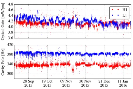
The optical responseCis tracked using a system known as the “photon calibrator,” which consists of an auxiliary Nd3þ∶YLF laser (operating at a wavelength of 1047 nm), an acousto-optic modulator, and a set of integrating spheres [38]. This calibration system actuates on the end test masses, applying a set of sinusoidal excitations via radi-ation pressure, to track variradi-ations of the optical gain and of

the differential coupled cavity pole frequency. Three weeks of such data are shown in Fig.4, showing that the optical response of the detectors is stable over time.

The absolute accuracy of the photon calibrator is limited by the uncertainties in its photodetector calibration, as well as any optical losses between the test mass and the photodetector. Overall, the uncertainty in the calibration of the interferometer over the entire operational frequency range from 10 Hz–1 kHz is estimated to be smaller than 10% and 10 degrees[39].

III. ANALYSIS OF THE INSTRUMENTAL NOISE

The calibrated gravitational wave signal is compared to the known noises in order to understand what limits the sensitivity of the instrument as a function of frequency. Figure5summarizes the noise contributions from various sources to the gravitational wave channel for the Livingston and Hanford detectors. The coupling of each noise source to the gravitational wave channel at a frequency f is estimated using the following equation:

LðfÞ ¼L₀hðfÞ ¼TðfÞ×NðfÞ; ð7Þ

whereNðfÞis the noise spectrum measured by an auxiliary (witness) sensor or computed using analytical model, and

TðfÞ is the measured or simulated transfer function from this sensor to the gravitational wave channel.

Noise sources can be divided into classes according to their origins and coupling mechanisms[10,40]. One clear way to differentiate noises is to split them into displacement and sensing noises: displacement noises cause real motion of the test masses or their surfaces, while sensing noises limit the ability of the instrument to measure test mass motion. However, this distinction is not perfect, since some noise sources (e.g., laser amplitude noise) can be assigned to both categories, as discussed in Sec.III E.

Another way to classify noise sources is to divide them into fundamental, technical and environmental noises. Fundamental noises can be computed from first principles, and they determine the ultimate design sensitivity of the instrument. This class of noises, which includes thermal and quantum noise, cannot be reduced without a major instrument upgrade, such as the installation of a new laser or the fabrication of better optical coatings. Technical noises, on the other hand, arise from electronics, control loops, charging noise and other effects that can be reduced once identified and carefully studied. Environmental noises include seismic motion, acoustic and magnetic noises. The design of Advanced LIGO calls for the contributions of technical and environmental noises to the gravitational wave channel to be small compared to fundamental noises. In practice, the sensitivity can be reduced due to unex-pected noise couplings. Many technical and environmental noises have been identified and are discussed in the following sections. At the same time, the dominant noise FIG. 4. Time-varying response of the Advanced LIGO

contributor in the frequency range 20–100 Hz has not yet been identified.

The narrowband features in the sensitivity plots shown in Fig.5 are caused by power lines (60 Hz and harmonics), suspension mechanical resonances, and excitations that are deliberately added to the instrument for calibration and alignment purposes. These very narrow lines are easily

excluded from the data analysis, while the broadband noise inevitably limits the instrument sensitivity. The latter is therefore a more important topic of investigation.

A. Seismic and thermal noises

Below 10 Hz, there is significant displacement noise from residual seismic motion. On average, at both the Livingston and Hanford sites, the ground moves by

∼10−9 _m=pffiffiffiffiffiffi_{Hzat 10 Hz—ten orders of magnitude larger}

than the Advanced LIGO target sensitivity at this fre-quency. To address this difference, seismic noise is filtered using a combination of passive and active stages. The test masses are suspended from quadruple pendulums [24]. These passive filters have resonances as low as 0.4 Hz and provide isolation as1=f8in the detection bandwidth. The pendulums are mounted on multistage active platforms [41,42]. These systems use very-low-noise inertial sensors to provide the required isolation in the detection band and at lower frequencies (below 10 Hz). This isolation is crucial for bringing the interferometer into the linear regime and allowing the longitudinal control system to maintain it on resonance. The active platforms combine feedback and feedforward control to provide one order of magnitude of isolation at the microseism frequencies (around 0.1 Hz) and three orders of magnitude between 1 Hz and 10 Hz. Most of the suspension resonances are located in this band, where ground excitation from anthropogenic noise and wind is significant.

Fluctuations of local gravity fields around the test masses—caused by ground motion and vibrations of the buildings, chambers, and concrete floor—also couple to the gravitational wave channel as force noise [43] (gravity gradient noise). The coupling to the differential arm length displacement is given by

LðfÞ ¼2NgravðfÞ

ð2πfÞ2

NgravðfÞ ¼βGρNseiðfÞ; ð8Þ

where N_grav is the fluctuation of the local gravity field projected on the arm cavity axis, the factor of 2 accounts for the incoherent sum of noises from the four test masses,Gis the gravitational constant,ρ≃1800kg m−3 is the ground density near the mirror,β≃10is a geometric factor, and

N_sei is the seismic motion near the test mass. Since the ground near the test masses moves by≃10−9m=pffiffiffiffiffiffiHz at 10 Hz, local gravity fluctuations at this frequency are

Ngrav≈10−15 m s−2=

ffiffiffiffiffiffi

Hz

p

and the total noise coupled into the gravitational wave channel at 10 Hz is

L≈5×10−19 m=pffiffiffiffiffiffiHz. Gravity gradient noise is one of the limiting noise sources of the Advanced LIGO design in the frequency range 10–20 Hz. However, the typical sensitivity measured during O1 is still far from this limitation.

(a) LIGO Livingston Observatory

(b) LIGO Hanford Observatory

Thermal noises arise from finite losses present in mechanical systems and couple to the gravitational wave channel as displacement noises. Several sources of thermal noise can be identified. Suspension thermal noise[44–46] causes motion of the test masses due to thermal vibrations of the suspension fibers. Coating Brownian noise is caused by thermal fluctuations of the optical coatings, multilayers of silica and titania-doped tantala[47–50]. The thickness of the coatings was optimized to reduce their thermal noise and provide the required high reflectivity of the mirrors [51,52]. Thermal noise also arises in the substrates of the test masses [53,54], but this effect is less significant. Thermal noise levels are analytically computed using the fluctuation-dissipation theorem[55]and independent mea-surements of the losses of the materials. The model predicts that thermal noise limits the Advanced LIGO design sensitivity in the frequency band 10–500 Hz, but is below the current noise floor by a factor of ≥3.

B. Quantum noise

Quantum noise is driven by fluctuations of the optical vacuum field entering the interferometer through the antisymmetric port [56,57]. This fundamental noise cou-ples to the interferometer sensitivity in two complementary ways[58]. For one, vacuum fluctuations disturb the optical fields resonating in the arm cavities, creating displacement noise by exerting a fluctuating radiation pressure force that physically moves the test masses[59,60]. The vacuum field is amplified by the optical cavities, and the noise seen in the differential arm channel is given by:

LðfÞ ¼ 2

cMπ2f2ðhνG−ParmÞ

1=2_K

−ðfÞ

LðfÞ ¼1.38×10

−17

f2

Parm

100kW

₁₌₂

K₋ðfÞ mffiffiffiffiffiffi

Hz

p ; ð9Þ

wherehis Planck constant in this section and Parm is the power circulating in the arm cavities. This “quantum radiation pressure noise” imposes a fundamental limit to the design sensitivity below 40 Hz, though it is still far from being a concern at the present operating power[23].

The vacuum fluctuations entering the interferometer through the antisymmetric port also introduce shot noise in the gravitational wave channel[61]. Vacuum fluctuations also mix with the main beam due to optical losses between the interferometer and the photodetector. In the current state of Advanced LIGO 25% of the power at the antisymmetric port is lost due to the output Faraday isolator, mode mis-match of the beam into the output mode cleaner cavity, and imperfect quantum efficiencies of the photodetectors. So the fraction of the interferometer output power that is transmitted to the photodiodes isη¼0.75.

Differential arm sensing noise due to shot noise on the photodetectors can be written as LðfÞ ¼L₀N_shot=CðfÞη,

where Nshot ¼ ð2hνηPLOÞ1=2 is the shot noise on the photodetector in units of W=pffiffiffiffiffiffiHz. The signal transfer functionCðfÞis determined by Eq.(6). The total shot noise is given by equations

LðfÞ ¼ λ

4πG_arm

2hνGsrc

G_prcP_inη

₁₌₂ 1

K₋ðfÞ

LðfÞ ¼2×10−20

100kW

Parmη

₁₌₂ 1

K₋ðfÞ

m

ffiffiffiffiffiffi

Hz

p : ð10Þ

The local oscillator power PLO cancels out in the final equation, and the shot noise level is independent of the differential arm offset for small offsetsΔL≲100pm.

The Advanced LIGO optical configuration is tuned to maximize power circulating in the arm cavities. The common coupled cavity build–up (ratio between the power resonating in the arms and power entering the interferom-eter) is related to the losses in the arm cavities by

G_comm≲ 1

2Y_arm; ð11Þ

whereY_armis round trip optical loss in one arm. During O1 the power circulating in the arm cavities wasGcomm≃5000 greater than the power entering the interferometer, corre-sponding to a round trip optical loss ofYarm≃100ppm in each arm cavity. The target optical gain for Advanced LIGO was 7500, which corresponds to round trip losses in the arm cavities of about 75 ppm. This number can possibly be achieved once the test masses are replaced after the second science run. The discrepancy in the round trip losses between the predicted and measured values is currently under study. Shot noise limits the design sensitivity above 40 Hz, and the current sensitivity above 100 Hz.

C. Gas noise

The Advanced LIGO optics are located inside vacuum chambers. The gas pressure in the corner station, where the dual-recycled Michelson interferometer is housed, and in the 4-km arm tubes, is maintained below 10−6 Pa. The presence of residual gas causes both displacement and sensing noise: thermal motion of gas molecules inside the vacuum chambers results in momentum exchange with the test masses via collisions; meanwhile, forward scattering of photons by the gas molecules in the arm tubes modulates the optical phase of the beam.

1. Squeezed film damping

estimated by applying the fluctuation-dissipation theorem or by running a Monte Carlo simulation[64]. The coupling coefficient depends on the gas pressure and the molecular mass, and it is found to be (below 100 Hz)

FðfÞ ¼1.5×10−14

p

10−6 _Pa

₁₌₂ m

m_H2

₁₌₄

N

ffiffiffiffiffiffi

Hz

p ; ð12Þ

wherepis the residual gas pressure in Pa, andmis the mass of a gas molecule. The calculated squeezed film damping noise shown in Fig. 5(a) is the sum of contributions from nitrogen (pN2≈6×10−7 Pa), hydrogen (pH2≈2×

10−6 _{Pa) and water (p}

H₂O≈10−7Pa).

2. Phase noise

Phase noise induced by the stochastic transit of mole-cules through the laser beam in the arm cavities, can be modeled by calculating the impulsive disturbance to the phase of the laser field as a gas molecule moves through the beam [65]. Such a model was used to estimate the high frequency part of the gas noise curve shown in Fig. 5(b). This estimation accounts for the pressure distribution in the arm cavities along with the profile of the laser beam, with the most significant noise contribution coming from the geometrical center of the tube, where the beam waist is located. The expected noise from residual gas is given by

LðfÞ ¼4×10−21N_gas mffiffiffiffiffiffi

Hz

p

N_gas¼

agas

a_H2

mgas

m_H2

₁₌₄ p

10−8 _Pa

₁₌₂

; ð13Þ

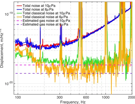
where a_gas is the polarizability of the gas molecules. The estimation of the gas phase noise was verified by changing the pressure in one of the arms by a factor of 3 at the end station and factor of 1.7 at the halfway point. The noise due to the residual gas pressure was estimated by measuring the change in the differential arm noise as shown in Fig.6. As discussed in Sec.III B, the noise above 100 Hz is limited by quantum shot noise, however, classical noises can be revealed by incoherent subtraction of shot noise from the measured signal. Using this technique, the classical noise was observed to change during this test as predicted by the model.

D. Charging noise

During the Advanced LIGO commissioning, it was discovered that the electrostatic actuation on the test masses was not symmetric among the four electrodes located on the reaction mass (see Fig.7). This mismatch in actuation strength is caused by electrostatic charge [66], which is distributed on the test masses in a nonuniform manner and has a slow time dependence.

Ideally, there should be no charge on the test masses, except for the one accumulated due to electrostatic actua-tion. However, some electric charge may be left by imperfect removal of the First Contact[67]polymer used for cleaning and protection of the optics. Moreover, surfaces of the test masses also lose electrons due to UV photons, generated by nearby ion pumps used in the vacuum system. Dust particles in the vacuum system provide yet another source of charging. It was discovered that the charge distribution changes on a∼week time scale. An order-of-magnitude estimate of the charge density on the front and back surfaces of the end test masses is σ∼10−11 _C=cm2_{. This number was estimated by exciting}

the electrodes and the potential of the ring heaters while measuring the longitudinal and angular motion of the test mass.

There are two coupling mechanisms of charging noise to the gravitational wave channel. The first mechanism arises due to interaction of the time varying charge with the metal cage around the test mass. The second coupling mechanism comes from voltage fluctuations of the various pieces of grounded metal in the vicinity of the test mass. Voltage noise creates fluctuations of the electric fieldEand applies a force F_ch on the test mass according to the following equation

100 300 600 1000 2000

Frequency, Hz

10-20 10-19

Displacement, m/Hz

1/2

Total noise at 10μPa Total noise at 6μPa Total classical noise at 10μPa Total classical noise at 6μPa Estimated gas noise at 10μPa Estimated gas noise at 6μPa

FIG. 6. Measurement of the gas phase noise for the two different pressures (average values are 10μPa and 6μPa) in one 4 km arm of the Livingston detector. The red and blue traces show total measured noise before and after the pump down. The dashed black curve shows the quantum noise level, which is independent of the pressure in the arms. The green and orange curves show total classical noise at pressure10μPa and6μPa correspondingly. The magenta and violet curves show the estimated gas phase noises. Reduction of classical noise is in agreement with the model that was used to compute gas phase noise. The gray curve shows other classical noises which do not depend on the gas pressure. Below 300 Hz there is an unknown

Fch¼ Z

EσdS; ð14Þ

where the integral is computed over both the front and back surfaces of the test mass. In this paper, we consider only the second coupling mechanism, since it is estimated to be the dominant one.

The broadband voltage noise on the ground plane is measured to be roughly 1 μV=pffiffiffiffiffiffiHz. This number was measured between the grounded suspension cage and the floating ring heaters. Since the characteristic distance between the test masses and the metal cage is 10 cm, the fluctuations in the electric field near the test mass are

∼10−5_ðV=mÞ=pffiffiffiffiffiffi_{Hz. The total noise coupling above 10 Hz}

is estimated using the equation

LðfÞ ¼ Fch

Mð2πfÞ2≈

10−16

f2

σ

10−11 _C=cm2

m

ffiffiffiffiffiffi

Hz

p : ð15Þ

The coupling of voltage fluctuations on the ground plane to the gravitational wave signal was reduced by a factor of 10–100 by discharging the test masses. Charge from the front surface can be efficiently removed using ion guns [68,69]: positive and negative ions are introduced into the chamber, when the pressure inside is ∼103 Pa, and anni-hilate surface charges on the front surface of the test mass. During the discharge procedure, it was found that the ions cannot efficiently reach the back surface due to the small gap between the test mass and the reaction mass, as shown in Fig. 7. The back surface of the end test masses was discharged by opening the chambers, separating the test and reaction mass, and directing an ion gun at close range toward the surfaces in the gap.

E. Laser amplitude and frequency noise

Advanced LIGO employs a Nd:YAG nonplanar ring oscillator as the main laser [19]. Intensity and frequency fluctuations of such a laser can be roughly approximated as 10−4=f=pffiffiffiffiffiffiHz and 104=fHz=pffiffiffiffiffiffiHz, respectively, in the frequency range 10 Hz–5 kHz. In the same band, the Advanced LIGO requirements are ∼10−8=pffiffiffiffiffiffiHz for intensity noise and ∼10−6 Hz=pffiffiffiffiffiffiHz for frequency noise.

In order to meet those requirements, a hierarchical control system is implemented. First of all, laser noises are actively suppressed using intensity and frequency stabilization servos. Additionally, laser noise on the beam entering the main interferometer is passively filtered by K_þ

Eq.(4) due to the common-mode coupled cavity pole. For laser amplitude noise, there are several coupling mechanisms. First of all, the presence of the nonzero differential arm offset △L needed for the homodyne readout means that the carrier light at the antisymmetric port is directly modulated by amplitude noise entering the interferometer. In addition, mismatches in the circulating arm powers and in the mirror masses also lead to intensity noise coupling through radiation pressure force at low frequencies (below 50 Hz).

Above 100 Hz, the most significant broadband coupling of laser amplitude noise comes from unequal effective lenses in the input test masses, due to substrate inhomo-geneity. The presence of imbalanced lenses creates a direct conversion of the fundamental laser field into higher-order spatial modes. As these modes do not resonate in the arm cavities, they are not filtered by the common-mode coupled cavity, and they therefore contribute to the coupling of laser intensity noise with a flat transfer function. A thermal compensation system (TCS)[70], which employs auxiliary CO₂ laser beams and ring-shaped heating elements, has been installed to compensate for such imbalances. Figure8 shows that the coupling of intensity noise can be signifi-cantly reduced by equalizing the substrate lenses using the TCS system: if no correction is applied, the differential lens power is40μD (micro diopter) and the coupling coefficient at 300 Hz is more than 40 dB larger than the lowest value attainable with a proper TCS correction.

Laser frequency noise is largely cancelled at the anti-symmetric port by virtue of the Michelson interferometer common-mode rejection (∼1000 at 100 Hz). However,

Reaction mass

Electrodes

Ring heater Suspension

cage HR coating

Test mass

FIG. 7. Top and front views of a test mass showing the arrangement of the electrodes, high reflective (HR) coating, ring heater and surrounding metal cage. Electrodes are used for actuation on the test mass. The ring heater is used to correct the curvature of the mirror.

100 300 600 1000 2000

Frequency, Hz

-60 -55 -50 -45 -40 -35 -30

Magnitude, dB

FIG. 8. Measured transfer function of intensity fluctuations from interferometer input to the antisymmetric port. The blue trace corresponds to the case when the lensing from the input test mass substrates are thermally matched. The red trace shows the coupling when the substrate lenses are different by7.5μD. For a difference of40μD the coupling above 60 Hz increases up to

residual frequency noise couples into the gravitational wave channel through the intentional asymmetry that is introduced into the Michelson interferometer to produce the necessary interference conditions for the rf control side-bands, and through imbalances in arm cavity reflectivities and pole frequencies[71,72]. The achieved laser frequency noise performance is limited primarily by sensing noises (shot noise, photodiode noise, and electronics noise) in the feedback control that stabilizes the laser frequency to the interferometer’s common (mean) arm length. In Advanced LIGO, noise in the frequency stabilization error signals limits the residual frequency noise of the beam entering the main interferometer to ≃10−6 Hz=pffiffiffiffiffiffiHz between 10 and 100 Hz, and increasing as f above 100 Hz.

F. Auxiliary degrees-of-freedom

The use of a dual-recycled Michelson interferometer optimizes the detector response to gravitational waves. Additionally, active control of the mirror angular degrees of freedom is important to stabilize the interferometer optical response. However, any noise in the associated auxiliary degrees of freedom will couple to the gravitational wave channel at some level. Figure9shows the typical noise in the auxiliary longitudinal degrees of freedom calibrated into displacement, as well as the typical angular noise in one of the arm cavity pitch degrees of freedom.

Any residual fluctuation of the Michelson lengthN_mich

couples to the transmitted power of the output mode cleaner, where the gravitational wave channel is trans-duced. The coupling mechanism is similar to that of a differential arm length fluctuation, but without the ampli-fication factor provided by the arm cavity build-up

G_arm¼270[40]:

LðfÞ ¼ 1

Garm

NmichðfÞ: ð16Þ

This coupling coefficient depends only weakly on the differential arm offset and alignment, unless the power buildup in the arm cavities is significantly changed (by more than 5%).

Residual fluctuations of the signal recycling cavity length also couple to the gravitational wave channel, due to the differential arm offset ΔL, through a radiation pressure force exerted on the test masses by the resonating optical fields. In the frequency range from 10 to 70 Hz, the differential arm noise LðfÞdue to signal recycling cavity longitudinal noiseNsrcl can be modeled as[73]

LðfÞ ¼0.16

f2

ΔL

10pmNsrclðfÞ; ð17Þ

where the numerical factor is determined mainly by the signal recycling mirror reflectivity and the masses of the cavity mirrors. Besides this linear coupling, a nonlinear

component appears due to low-frequency modulation of the differential arm offset ΔL (by ∼10–20%), which arises from unsuppressed angular motion of the interferometer mirrors. Such motion generates higher-order mode content in the beam exiting the interferometer through the anti-symmeteric port, leading to modulation of the power transmitted by the output mode cleaner and forcing the differential arm length servo to compensate by changing the offset ΔL. At higher frequencies (above 70 Hz), the coupling of the signal recycling cavity longitudinal noise depends on the mode matching between the signal recy-cling cavity and the arm cavities. This can be tuned using the thermal compensation system discussed above.

The coupling of the power recycling cavity length to the differential arm channel is caused by imbalances in the two arm cavities and cross couplings with other longitudinal degrees of freedom. Residual power recycling cavity length noise is less significant (by a factor of ≥10) compared to other degrees of freedom of the dual-recycled Michelson interferometer.

Finally, any residual angular motion of the test masses

N_ang couples to the gravitational wave channel geometri-cally due to beam miscenteringdon the mirrors, according to the equation

LðfÞ ¼d×NangðfÞ: ð18Þ

The beam miscentering itself is also modulated by the mirror angular motion d¼d¯ þdac, where d¯ and dac∝ Nang are stationary and nonstationary components of the beam position. For this reason, the coupling of the angular motion can be linear and nonlinear. The angular feedback servos are optimized to suppress low-frequency motion of the cavity axis andd_ac while avoiding injection of sensor noise at high frequencies.

The linear coupling of the auxiliary degrees of freedom to the gravitational wave channel is mitigated using a realtime feed-forward cancellation technique. Witness sig-nals are properly reshaped using time-domain filters, and the cancellation signals are applied directly to the test masses. This feed-forward scheme significantly reduces the contribution of noise in auxiliary degrees of freedom to the gravitational wave channel in the frequency range 10–150 Hz. The typical subtraction factors for Michelson length noise, signal recycling cavity length noise, and angular noise are 30, 7 and 20, respectively.

G. Oscillator noise

The rf oscillator used to generate the Pound-Drever-Hall control sidebands has phase and amplitude noise, and these couple to the gravitational wave channel via both sensing intensity noise and displacement noise in the dual-recycled Michelson degrees of freedom.

power contained in the rf sidebands. Since the total power in the carrier and the rf sidebands is actively controlled, fluctuations in the rf sideband field amplitudes produce fluctuations in the carrier field amplitude (i.e., audio sidebands). These audio sidebands propagate through the interferometer and couple into the gravitational wave channel via the same mechanisms as laser intensity noise as discussed in Sec.III E. Additionally, as intensity noise of rf sidebands is not filtered by the common coupled cavity pole and the output mode cleaner has a finite attenuation at the rf sideband frequencies (≃6×10−5 W=W for the

45 MHz sidebands), a small amount of sideband power fluctuations appears directly on the GW readout photo-diodes. The oscillator amplitude noise coupling for the 9 MHz and 45 MHz sidebands was measured to be

LðfÞ ¼5×10−22

N9amp

10−6

1

K₋ðfÞ

m

ffiffiffiffiffiffi

Hz

p

LðfÞ ¼5×10−21

N45amp

10−6

1

K₋ðfÞ

m

ffiffiffiffiffiffi

Hz

p ; ð19Þ

101 102 103

Frequency, Hz 10-18 10-17 10-16 10-15 10-14 10-13 10-12 Displacement, m/Hz 1/2 Measured noise Seismic noise Suspension damping Thermal noise Dark noise Quantum noise Actuator noise Expected noise

101 102 103

Frequency, Hz 10-18 10-17 10-16 10-15 10-14 10-13 10-12 Displacement, m/Hz 1/2 Measured noise Seismic noise Suspension damping Thermal noise Dark noise Quantum noise Actuator noise Beam splitter motion Expected noise . h t g n e l y t i v a c g n i l c y c e r r e w o P ) b ( . h t g n e l n o s l e h c i M ) a (

101 102 103

Frequency, Hz 10-17 10-16 10-15 10-14 10-13 10-12 Displacement, m/Hz 1/2 Measured noise Seismic noise Suspension damping Thermal noise Dark noise Quantum noise Actuator noise Beam splitter motion Expected noise

Frequency, Hz

10-2 10-1 100 101 102

Pitch, rad/Hz 1/2 10-18 10-16 10-14 10-12 10-10 10-8 10-6 Residual motion RMS of residual motion Control signal RMS of control signal

. ) h c t i p ( n o i t o m r a l u g n a s s a m t s e T ) d ( . h t g n e l y t i v a c g n i l c y c e r l a n g i S ) c (

where N9amp and N45amp is the relative amplitude noise of 9 MHz and 45 MHz sidebands in units of 1=pffiffiffiffiffiffiHz.

Oscillator phase noise is converted to rf sideband amplitude noise through any optical path length imbalance in the interferometer’s Michelson degree of freedom. The main sources of imbalance are the intentional asymmetry in the Michelson interferometer and a transmissivity differ-ence of the input test masses (which produces a differential phase delay when the sidebands are reflected from each arm) [72]. The oscillator phase noise coupling for the 9 MHz and 45 MHz sidebands was measured to be

LðfÞ ¼10−21

_N9 phf

10−2

1

K₋ðfÞ

m

ffiffiffiffiffiffi

Hz

p

LðfÞ ¼10−22

_N45 phf

10−2

1

K₋ðfÞ

m

ffiffiffiffiffiffi

Hz

p ; ð20Þ

where N9_ph and N45_ph are the relative phase noises of the 9 MHz and 45 MHz sidebands in units of 1=pffiffiffiffiffiffiHz.

H. Beam jitter

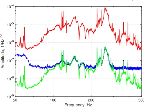
Pointing fluctuations, quantified by the factor Δw=w, wherewis the beam size andΔwis the transverse motion of the beam, are also a source of noise. On the input side, significant beam jitter is caused by angular and longitudinal motion of the steering mirrors, located in air. The input mode cleaner, located in vacuum, attenuates the input beam jitter by a factor of≃150. Figure10shows the relative pointing fluctuations before and after the input mode cleaner.

Residual input beam jitter is converted into intensity fluctuations by the interferometer resonant cavities: the power and signal recycling cavities, the arm cavities, and finally the output mode cleaner cavity. In the frequency range 100–1000 Hz, the coupling coefficient from relative pointing noise at the interferometer input to the relative intensity noise at the antisymmetric port is∼0.01.

Figure5shows that the contribution of the beam jitter is close to the measured strain noise at a few peaks between 200 and 600 Hz. These structures in the noise are due to resonances of mirror mounts in the in-air input beam path. This contribution has been reduced by improving the stiffness of the optical elements, thus reducing the motion. On the output side, beam jitter is caused by angular motion of the output steering mirrors. These are single pendulum stage suspended optics, located in vacuum, on vibration isolated platforms. While the interferometer alignment is actively controlled to reduce beam jitter, any residual angular motion modulates the power trans-mitted by the output mode cleaner and thereby couples to the gravitational wave channel.

I. Scattered light noise

The motion of the suspended optics is significantly less than that of the ground, as discussed in Sec.III A. However,

the vacuum chambers and arm cavity beam tubes are not isolated from the seismic or the ambient acoustic noises. This motion can couple to the gravitational wave channel through backscattered light.

A small portion of the laser light scatters out of the main beam when it hits the optical components. Part of this light is scattered back from the moving chamber walls, baffles, mirrors, or photodiodes, and couples into the main beam as shown in Fig.11. Backscattered light modulates the main beam in phase and amplitude, and introduces noise into the gravitational wave channel. The phase modulation is directly detected at the antisymmetric port, and amplitude modulation moves the test masses by means of radiation

50 100 200 500

Frequency, Hz

10-9 10-8 10-7 10-6 10-5 10-4

Amplitude, 1/Hz

1/2

FIG. 10. Relative pointing noise before and after the input mode cleaner in the L1 interferometer. Acoustic peaks in the L1 and H1 interferometers are at slightly different frequencies. The red trace shows the spectrum measured before the input mode cleaner, where the laser beam enters the vacuum system. The blue trace shows the measured jitter after the input mode cleaner. This measurement is limited by the sensing noise of the quadrant photodetector at a level of4×10−8=pffiffiffiffiffiffiHz. The green trace is the estimated relative pointing noise used in the calculation of the jitter coupling to the gravitational wave channel. This curve is computed by dividing the red spectrum by the filtering coefficient of the input mode cleaner.

Input test mass

4km

1m End test mass

pressure. Significant scattering processes occur inside the arm cavities, at the input and output ports, and in the recycling cavities.

1. Beam tubes

Light scattered out from the main beam by the test masses couples motion of the 4 km beam tube to the gravitational wave channel. The bidirectional reflectivity distribution function (BRDF) of the test masses depends on the imperfections in the mirror surface. If the wavelength of a coating ripple isλr, then the angle between the scattered light and the main beam isθ¼λ=λr. The amount of power scattered out from the main beam depends on the amplitude of the ripple. The fractional power scattered out in the cone with half angleθ≪1 and widthdθ is given by:

dP_s

Parm

≈

4π

λ

₂

Sdθ

λ ¼BRDFm×dΩ ð21Þ

whereSðθ=λÞ ¼Sðλ−r1Þis the power spectral density of the coating aberrations[74,75], anddΩ¼2πθdθis solid angle of scattering. For θ∼1, the BRDF can be approximated as BRDF_m ¼3×10−6cosðθÞsr−1.

Light scattered out from the main beam hits a baffle in the beam tube and scatters back into the main beam. The measured BRDF of the baffle at large angles is BRDFb¼0.02sr−1. In order to get back into the main beam, light from the baffle scatters into the solid angle λ2_=r2_{× BRDF}

m [76], where r is the distance from the baffle to the test mass. The total optical power Pr that recombines with the main beam is determined by the following equation[77]:

dP_r

Parm

¼λ2

r2BRDF

2

mBRDFbdΩ: ð22Þ

The coating profiles were measured [23] and can be approximated as a smooth polynomial function in the wide range ofλrfor narrow angle scattering. However, the high-reflectivity coatings applied on the end test masses show a distinct azimuthal ripple in the coating surface height. The spatial wavelength of the ripple is 7.85 mm and its maximum amplitude is 1 nm pk-pk. This ripple is located at radii beyond about 3 cm from the mirror center and significantly contributes to the scattered light noise [78]. The total scattered light noise contribution to the differ-ential arm channel from the tube motion N_tube is

LðfÞ ¼

ffiffiffiffiffiffiffiffiffiffiffiffiffiffiffi 2

R

dPr

P_arm

s

N_tubeðfÞ≈10−11N_tubeðfÞ; ð23Þ

where the integral is computed over all scattering angles (the factor of 2 accounts for the incoherent sum of all four test masses and for the fact that1=2of the baffle motion, in

power, is in the phase quadrature of the main field). Equation (23) accounts only for the phase quadrature and ignores radiation pressure noise. This is a valid assumption for the current optical powerP_arm≈100kW. The estimated scattered light noise, coming from the arm cavities, is a factor of 30–100 below the current sensitivity of the interferometer. This result was confirmed by apply-ing periodic mechanical excitation to the beam tube at different frequencies and measuring the response in the gravitational wave channel.

2. Vacuum chambers

Similar scattering processes occur in the chambers and short tubes in the corner station, where the dual-recycled Michelson interferometer is located. One method to assess the contribution of scattering noise to the detector back-ground is to inject known acoustic signals and measure the response in the gravitational wave channel[79]. In general, coupling of scattered light noise is not linear but rather modulated by the low frequency motion of the scattering surfaces. For this reason, instead of measuring the transfer function from the excitation to the sensor, we monitor excess power in the signal spectrum. Then we make a projection of scattered light noise to the gravitational wave channel according to the following equation

LðfÞ ¼NambðfÞ

LexcðfÞ

N_excðfÞ; ð24Þ

where Lexc and Nexc are the spectra of the gravitational wave channel and of the back scattering element motion, respectively, when an excitation to the element is applied, andN_amb is the motion of the scattering element without any excitation. Figure12shows that the projected ambient acoustic noise coupling to the gravitational wave channel is below the measured sensitivity.

3. Fringe wrapping

RINðtÞ ¼2rcosð4πN_omcðtÞ=λÞ; ð25Þ

where r¼10−5–10−4 is the effective field reflectivity of the interferometer output port andNomcðtÞis the distance fluctuation between the interferometer and the output mode cleaner. Since this distance is not controlled, the amplitude ofNomcðtÞcan be as large as several wavelengths, and the cosine in the above equation wraps this rapidly varying phase between 0 and 2π, leading to up-conversion of the low frequency motion of the length. The resulting“ scatter-ing shelves”are seen in the differential arm length spectrum with a cutoff frequency of2=λ×dNomc=dt. In Advanced LIGO, when the micro-seismic motion is higher than normal, this process increases the gravitational wave channel noise below 20 Hz[73]. Figure13shows scattering shelves in the gravitational wave channel during the low frequency modulation of the distance N_omc.

J. Sensing and actuation electronics noise

This section summarizes noise contributions from elec-tronic circuits in photodetectors, actuators, analog-to-dig-ital (ADC) and diganalog-to-dig-ital-to-analog (DAC) converters and whitening boards, all of which are essential for sensing optical signals and actuating on suspensions. From a design perspective, all electronics noise should be smaller than fundamental noises.

For the differential arm length signal, a pair of reverse-biased InGaAs photodiodes, equipped with in-vacuum preamplifiers, measures the light transmitted by the output mode cleaner. Subsequently, these signals are acquired by a digital system through analog-to-digital converters, further dividing sensing noise into two types: dark noise and ADC

noise. Dark noise includes any dark current produced by the photodiodes, Johnson-Nyquist noise of the readout transimpedance, and noise in all other downstream analog electronics. A current noise level of ∼10pA=pffiffiffiffiffiffiHz, at 100 Hz, is present in each photodetection circuit, equivalent to the shot noise of a DC current of 0.3 mA. This can be compared against the actual operating current of 10 mA. Taking the coherent sum of two photodetectors into account, we estimate the dark noise to be a factor of 8.2 lower than the shot noise at 100 Hz, as shown in Fig.5. ADC input noise is suppressed by inserting additional analog gain and filtering, referred to as“whitening filters.” An offline measurement of the ADC noise shows that it is below the current best noise level by a factor of more than 10 over the entire measurement frequency band.

The other important noise in this category is noise in the actuation used to apply feedback control forces on the mirrors. Any excess noise at the level of the required actuation couples directly to mirror displacement. The most critical actuation noise is due to the digital-to-analog convertors that bridge the digital real-time control process and the analog suspension drive electronics. It is a significant challenge to achieve both the high-range actua-tion, needed to bring the interferometer into the linear regime from an uncontrolled state (lock acquisition)[30], and low-noise actuation for operation in the observation state. This issue has been tackled by installing a gain-switchable force controller, which has several operational states. After the interferometer is brought into the linear regime, the controller state is changed from the high-dynamic-range to the low-noise state. Also, noise from the digital-to-analog converter is mechanically filtered via the suspension force-to-displacement transfer function above

∼0.5Hz. The current estimate puts the actuation noise as low as3×10−18 m=pffiffiffiffiffiffiHz at 10 Hz.

20 100 1000 5000

Frequency, Hz

10-22 10-21 10-20 10-19 10-18

Displacement, m/Hz

1/2

GW signal channel End X buliding End Y building

Corner Station Center and Output Area Corner Station Input Area

Laser Enclosure

FIG. 12. Projected contribution of the ambient acoustic noise to the gravitational wave channel. An acoustic excitation was applied at different locations near the vacuum chambers: near the end test masses of both arm cavities (X and Y), near the dual-recycled Michelson interferometer (corner station), and near the main laser.

101 102

Frequency, Hz

10-20 10-19 10-18 10-17 10-16 10-15

Displacement, m/Hz

1/2

Lastly, active damping of the suspension systems is known to introduce noise. Below 5 Hz, the high-Q suspension resonances are damped by sensing the motion of the suspension relative to its support using shadow sensors[25]. According to dynamical suspension models, noise from the local damping control is estimated to be

2×10−18 m=pffiffiffiffiffiffiHz at 10 Hz, and rapidly decreases at higher frequencies.

K. Noise stationarity

A common figure of merit for ground-based interfero-metric detectors is their sensitivity to the inspiral of two neutron stars, averaged over relative orientations of the binary system and sky locations at a nominal SNR thresh-old of 8. A plot of the sensitivity of the LIGO detectors to signals of this type is given in Fig. 14, over a one month time scale.

If the sum of all the noises is truly Gaussian and stationary, the strain noise density at a given frequency will vary randomly in time following a Rayleigh distribu-tion. In Fig.15, we compare the 95th and 99.7th percentiles of the noise in each frequency bin to the expectation for stationary Gaussian noise. Deviations from the expectation are due to nonstationary noises (e.g., transient environ-mental disturbances that generate very short-duration bursts of excess noise, mostly at low frequency) or narrowband features that are coherent over long time scales. Above 100 Hz, the deviation from stationary Gaussian noise is small. Below 100 Hz, the fluctuations can mask or mimic gravitational waves and must be addressed by further commissioning and, for O1 data, through vetoes that are applied following data collection and analysis.

The characterization and mitigation of the detector stationary noise and noise transients is the focus of a large

collaborative effort between instrument specialists and the gravitational wave data analysis community[81,82].

IV. CONCLUSIONS

The first Advanced LIGO observational run (O1) started in September 2015 and concluded in January 2016. The observatory was running at unprecedented sensitivity to gravitational waves in the frequency range 10 Hz–10 kHz. The average distance at which Advanced LIGO could detect the coalescence of binary black hole systems with individual masses of30M_⊙ and with signal-to-noise ratio of 8 was 1.3 Gpc. The reach for binary neutron star inspirals during the first science run was about 75 Mpc.

The commissioning of Advanced LIGO lasted for

∼1year before the beginning of O1. During this period, a variety of technical noise sources was discovered and eliminated. In this paper, we discussed the dominant noise sources that limited Advanced LIGO sensitivity during the first science run. The coupling of auxiliary degrees of freedom, laser amplitude noise, suspension actuation and other technical noises considered in this paper were significantly reduced.

Future work is required to find the remaining noise sources. In particular, below 100 Hz, the sum of all known noise sources in the gravitational wave channel could not explain the measured sensitivity curve.

Above 100 Hz, the Advanced LIGO sensitivity was limited mostly by photon shot noise. For this reason, one certain activity on the commissioning agenda is to increase the interferometer input power and ultimately to introduce squeezed states of light[61,83,84]. During the first science run, Advanced LIGO operated in the low power regime: input power was 25 W out of maximum laser power of ≃180W. A set of technical difficulties must be overcome FIG. 14. Sensitivity of the two Advanced LIGO detectors to

binary neutron star inspirals, averaged over sky position and orientation and 1 minute of data. The sensitivity drop in the L1 interferometer at the end of the run was caused by electronics noise at one of the end stations. This noise was identified and eliminated shortly after the observing run.

101 ₁₀2 ₁₀3

Frequency [Hz] 1

2 3 4 5 6 7

Strain

A

SD,

Normalized

to

Median

H1 3σ H1 2σ L1 3σ L1 2σ

Gaussian Noise 3σ Gaussian Noise 2σ