City, University of London Institutional Repository
Citation
:
Li, S., Fairbank, M., Johnson, C., Wunsch, D. C., Alonso, E. and Proano, J. L.
(2013). Artificial Neural Networks for Control of a Grid-Connected Rectifier/Inverter Under
Disturbance, Dynamic and Power Converter Switching Conditions. IEEE Transactions on
Neural Networks and Learning Systems, 25(4), pp. 738-750. doi:
10.1109/TNNLS.2013.2280906
This is the accepted version of the paper.
This version of the publication may differ from the final published
version.
Permanent repository link:
http://openaccess.city.ac.uk/5179/
Link to published version
:
http://dx.doi.org/10.1109/TNNLS.2013.2280906
Copyright and reuse:
City Research Online aims to make research
outputs of City, University of London available to a wider audience.
Copyright and Moral Rights remain with the author(s) and/or copyright
holders. URLs from City Research Online may be freely distributed and
linked to.
City Research Online:
http://openaccess.city.ac.uk/
publications@city.ac.uk
Abstract -- Three-phase grid-connected converters are widely used in renewable and electric power system applications. Traditionally, grid-connected converters are controlled with standard decoupled d-q vector control mechanisms. However, recent studies indicate that such mechanisms show limitations in their applicability to dynamic systems. This paper investigates how to mitigate such restrictions using a neural network to control a grid-connected rectifier/inverter. The neural network implements a dynamic programming algorithm and is trained by using backpropagation through time. To enhance performance and stability under disturbance, additional strategies are adopted, including the use of integrals of error signals to the network inputs and the introduction of grid disturbance voltage to the outputs of a well-trained network. The performance of the neural network controller is studied under typical vector control conditions and compared against conventional vector control methods, which demonstrates that the neural vector control strategy proposed in this paper is effective. Even in dynamic and power converter switching environments, the neural vector controller shows strong ability to trace rapidly changing reference commands, tolerate system disturbances, and satisfy control requirements for a faulted power system.
Index Terms – neural controller, dynamic programming, backpropagation through time, grid-connected rectifier/inverter, decoupled vector control, renewable energy conversion systems
I. INTRODUCTION
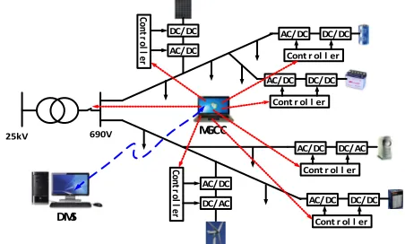
N renewable and electric power system applications, a three-phase grid-connected dc/ac voltage-source pulse-width-modulated (PWM) converter is usually employed to interface between the dc and ac systems. Typical converter configurations containing the grid-connected converter (GCC) include: 1) a dc/dc/ac converter for solar, battery and fuel cell applications [1, 2], 2) a dc/ac converter for STATCOM applications [3, 4], and 3) an ac/dc/ac converter for wind power and HVDC applications [4-8]. Figure 1 demonstrates
This work was supported in part by the U.S. National Science Foundation under Grant EECS 1059265/1102159, the Mary K. Finley Missouri Endowment, and the Missouri S&T Intelligent Systems Center.
Shuhui Li and Julio Proano are with the Department of Electrical & Computer Engineering, The University of Alabama, Tuscaloosa, AL 35487, USA (email: sli@eng.ua.edu, jlproano@crimson.ua.edu).
Michael Fairbank and Eduardo Alonso are with the School of Informatics, City University London, UK (email: michael.fairbank@virgin.net, e.alonso@city.ac.uk).
Donald C. Wunsch, the Mary K. Finley Missouri Endowment professor, and Cameron Johnson are with the Department of Electrical & Computer Engineering, Missouri University of Science and Technology, Rolla, MO 65409-0040, USA (email: dwunsch@mst.edu, cej@mst.edu).
the grid-connected dc/ac converter used in a microgrid to connect distributed energy resources. Conventionally, this type of converter is controlled using the standard decoupled d-q vector control approach [5-8].
25kV 690V
AC/DC DC/DC DC/DC
AC/DC
Co
nt
ro
ll
er Cont r ol l er
AC/DC DC/DC
Cont r ol l er
AC/DC DC/DC
Cont r ol l er AC/DC DC/AC
Cont r ol l er AC/DC
DC/AC
Co
nt
ro
ll
er
MGCC
[image:2.612.331.557.240.376.2]DMS
Fig. 1. Application of grid-connected rectifier/inverter in a microgrid
Notwithstanding its merits, recent studies indicate that this control strategy is inherently limited due to its competing nature [9, 10]. Issues reported in the literature include: i) difficulty in tuning the proportional-integral (PI) controllers [3], ii) instability in low voltage applications [11], iii) fluctuating dc-link voltage [12], iv) malfunction such as unexpected trips [5], and v) difficulty to synchronize for initial connection of the GCC to the electric power grid [13].
For example, in [3], it is noted that tuning PI parameters for a standard decoupled d-q vector controller in a STATCOM application is difficult. This finding is consistent with a result reported in this paper, which shows that tuning the PI gains is hard at a large sampling time. [14]-[16] show that the inner-current controller and the phase-locked loop dynamics of conventional control techniques may be affected significantly in weak ac-system connections. [11] also informs of instable operability in such conditions. [12] indicates that there is a high fluctuating dc-link voltage using the conventional GCC control approach. [5], [17] and [18] show that wind farms periodically experience a high degree of imbalance and harmonic distortions, which has resulted in numerous trips. [13] and [19] point out that using conventional vector control methods, synchronization is always required for initial connection of a GCC to the electric power grid. [20] and [21] indicate that the poor performance of such technology has become an obstacle for GCCs in HVDC transmission under challenging ac-system conditions.
To overcome the deficiencies, an adaptive control approach was proposed recently that employs a direct-current
Artificial Neural Networks for Control of a Grid-Connected
Rectifier/Inverter under Disturbance, Dynamic and Power
Converter Switching Conditions
Shuhui Li, Michael Fairbank, Cameron Johnson, Donald C. Wunsch, Eduardo Alonso, and Julio Proano
control (DCC) strategy [22, 23]. However, a major challenge of the direct-current-based vector control mechanism is that no well-established systematical approach to tuning the PI controller gains exists, so that optimal DCC is hard to obtain. Other control methods have also been developed recently, direct power control [24-26] and predictive current control [27-29] in particular. Notwithstanding their merits, all these control methods show some limitations. This situation motivates the development of neural-network based optimal control techniques for GCC vector control applications, as presented in this paper.
In recent years, significant research has been conducted in the area of dynamic programming (DP) for optimal control of nonlinear systems [30-34]. Classical DP methods discretize the state space and directly compare the costs associated with all feasible trajectories that satisfy the principle of optimality, guaranteeing the solution of the optimal control problem [35]. Adaptive critic designs constitute a class of approximate dynamic programming (ADP) methods that use incremental optimization combined with parametric structures that approximate the optimal cost and the control [36-38]. Both classical DP and ADP methods have been used to train neural networks for many nonlinear control applications, such as steering and controlling the speed of a two-axle vehicle [39], intercepting an agile missile [40], performing auto landing and control of an aircraft [41-43], controlling a turbogenerator [44], and tracking control with time delays [45]. As for GCC controllers, neural networks have been primarily used to generate external reference signals. In [46], a neuro-fuzzy external controller is developed to generate reference ac bus voltage signal to the PI controller of a STATCOM for coordinated optimal control of the STATCOM and two synchronous generators. In [47], an interface neuro-controller is proposed for coordinated reactive power control between a large wind farm equipped with doubly fed induction generators (DFIGs) and a STATCOM, while the GCC controllers within both DFIGs and the STATCOM have adopted conventional standard PI vector control structures.
In [48], we developed a preliminary neural network vector control structure for GCCs in renewable and electric power system applications. However encouraging the results were, the design showed steady-state errors and was unable to track targets properly under variable system parameters. This paper has extended far beyond [48] by developing an improved neural network design to overcome these limitations and by testing the neural vector control strategy in a more practical nested-loop control condition. Moreover, a control signal can only be applied to an actual system through power converters, which involves continuous switching on and off of the converters [49] and hence distorts the ideal control signal. This switching impact is carefully evaluated in this paper.
The rest of the paper is structured as follows. The basic topologies of the standard vector control method, DCC, DPC and PCC are briefly evaluated in Section II. Section III proposes a neural network vector control configuration. Section IV explains how to employ dynamic programming to achieve optimal neural vector control for the GCC system.
The performance of the neural network vector control scheme is assessed in dynamic and power converter switching environments in Section V. Section VI analyzes the performance of the neural vector controller in a nested-loop control condition. Finally, the paper concludes with a summary of the main points.
II. CONVENTIONAL GCCCONTROL TECHNIQUES
Figure 2 shows the schematic of the GCC, in which a dc-link capacitor is on the left, and a three-phase voltage source, representing the voltage at the Point of Common Coupling (PCC) of the ac system, is on the right.
C
+
-Vdc
va
vc vb
R L
va1
vb1
vc1
ia
ib ic
Fig. 2. Grid-connected converter schematic
In the d-q reference frame, the voltage balance across the grid filter is:
1
1
d d d q d
s
q q q d q
v i d i i v
R L L
v i dt i
ω
i v−
⎡ ⎤= ⎡ ⎤+ ⎡ ⎤+ ⎡ ⎤+⎡ ⎤
⎢ ⎥ ⎢ ⎥ ⎢ ⎥ ⎢ ⎥⎣ ⎦ ⎢ ⎥
⎣ ⎦ ⎣ ⎦ ⎣ ⎦ ⎣ ⎦ (1)
where ωs is the angular frequency of the grid voltage, and L
and R are the inductance and resistance of the grid filter. In the PCC voltage-oriented frame [3, 50], the instant active and reactive powers absorbed by the GCC from the grid are proportional to the grid's d- and q-axis currents, respectively, as shown by Eqs. (2) and (3).
( )
d d q q d dp t
=
v i
+
v i
=
v i
(2)( )
q d d q d qq t
=
v i
−
v i
=
−
v i
(3)A. Standard Vector Control
The standard vector control method for the GCC, widely used in renewable and electric power system applications, deploys a nested-loop structure consisting of a faster inner current loop and a slower outer loop, as shown in Fig. 3 [3, 4, 50]. In this figure, the d-axis loop is used for dc-link voltage control, and the q-axis loop is used for reactive power or grid voltage support control. The control strategy of the inner current loop is developed by rewriting Eq. (1) as:
(
)
1
d d d s q d
v
=
−
Ri
+
L di dt
⋅
+
ω
Li
+
v
(4)(
)
1
q q q s d
v
=
−
Ri
+
L di dt
⋅
−
ω
Li
(5)
Fig. 3 Standard vector control structure
B. Direct-Current Vector Control (DCC)
The DCC [22, 23], developed recently to overcome the deficiencies of standard vector control techniques, is considered as a pilot adaptive vector control strategy. The theoretical foundation of the DCC is expressed in Eqs. (2) and (3), i.e., the use of d- and q-axis currents directly for active and reactive power control of the GCC system. Unlike the conventional approach that generates a d- or q-axis voltage from a GCC current-loop controller, the DCC outputs a current signal by the d- or q-axis current-loop controller (Fig. 4). In other words, the output of the controller is a d- or q-axis tuning current i'd or i'q, while the input error signal tells the
controller how much the tuning current should be adjusted during the dynamic control process. The development of the tuning current control strategy has adopted intelligent control concepts [23], e.g., a control goal to minimize the absolute or root-mean-square (RMS) error between the desired and actual d- and q-axis currents through an adaptive tuning strategy. Nonetheless, a major challenge of the DCC is that no well-established systematical approach exists for tuning the controller PI gains, so an optimal DCC controller is difficult to obtain. Actually, the cross terms as shown in Fig. 4 imply that a neural network vector controller could be a better fit to meet the GCC control requirements.
Fig. 4. GCC direct-current vector control structure
C. Direct Power Control (DPC)
The basic idea of the Direct Power Control approach, proposed by Noguchi [24], is the direct control of active and reactive power. In DPC, the inner current control loops and the PWM modulator are not required because the converter switching states are selected by a switching table based on the instantaneous errors between the commanded and the estimated values of active and reactive powers (Fig. 5). The active and reactive power errors are fed to hysteresis comparators and their outputs, together with the system’s vector phase, are used to select from the switching tables the best vector for the next control cycle. DPC has the advantages of high dynamic response to demands in active or reactive power and simplicity in implementation [25, 26]. But, primary disadvantages of this control technique are high harmonic distortion and unbalance in the system current, variable
switching frequency under different operating conditions, and requirement of a high switching frequency [26], which causes major impacts to a GCC system.
[image:4.612.325.544.94.191.2]
Fig. 5. Direct power control configuration
D. Predictive Current Control (PCC)
The predictive control algorithm first estimates the model parameters, including R and L of the grid filter and PCC voltage [27]. The model is then used to predict the current and to determine the voltage necessary to meet the control objective for each control interval. In Fig. 6, the PCC block involves a current prediction equation to estimate the grid current at the next sampling interval and a control equation to determine the next GCC control voltage [27, 28].
A PCC has a fast current tracking response, which permits the minimization of the dc-bus capacitance, increases the voltage loop bandwidth, and reduces harmonic distortions in ac current waveforms [28, 29]. But, a PCC becomes unstable when the programmed filter inductance differs from its actual value. In addition, if the resistive part of the filtering inductors is not accurately measured and programmed, the predictive control presents a steady-state error. Since filter parameters vary along with inverter operation, it is difficult to achieve an adequate static and dynamic performance [29].
In summary, in order to meet to the optimal GCC control requirements it is important to develop new methods that integrate the advantages of different conventional control techniques and at the same time avoid their shortcomings. Our neural network controller proposal is a step in that direction.
Fig. 6. Predictive current vector control structure
III. STRUCTURE OF GCCVECTOR CONTROL USING
ARTIFICIAL NEURAL NETWORKS
The neural-network-based vector control structure of the GCC current-loop is shown in Fig. 7, in which the converter output voltage, grid PCC voltage, and grid current are consistent with those shown in Fig. 2. The neural network, known here as the action network, is applied to the GCC through a PWM mechanism to regulate the GCC output
PI V*
dc Vdc
+
- i*
d
PI id
+
- v’
d
-ωsL⋅iq +
v* d1
PI V*
bus Vbus
+
- i*
q
PI iq
+
- v’
q
-ωsL⋅id
-v* q1 vd
[image:4.612.70.268.449.537.2] [image:4.612.341.529.515.615.2]voltage va1,b1,c1 in the three-phase ac system. The ratio of the
GCC output voltage to the output of the action network is a gain of kPWM, which equals to Vdc/2 if the amplitude of the
triangle voltage waveform in the PWM scheme is 1V [49]. The integrated GCC and grid system is described by Eq. (1), which is rearranged into the standard state-space representation as shown by Eq. (6), where the system states are id and iq, grid PCC voltages vd and vq are normally
constant, and converter output voltages vd1 and vq1 are the
control voltages that are to be specified by the output of the action network. For digital control implementation and the offline training of the neural network, the discrete equivalent of the continuous system state-space model from Eq. (6) must be obtained [51] as shown by Eq. (7), where Ts represents the
sampling period, k is an integer time step, F is the system matrix, and G is the matrix associated with the control voltage. In this paper, a zero-order-hold discrete equivalent is used to convert the continuous state-space model of the system in Eq. (6) to the discrete state-space model in Eq. (7). We used
Ts=1ms in all experiments.
1
1
1 1
d f f s d d d
q s f f q f q f q
i R L i v v
d
i R L i v v
dt L L
ω
ω
−
⎡ ⎤ ⎡ ⎤ ⎡ ⎤ ⎡ ⎤ ⎡ ⎤
=− − +
⎢ ⎥ ⎢ ⎥ ⎢ ⎥ ⎢ ⎥ ⎢ ⎥
⎣ ⎦ ⎣ ⎦ ⎣ ⎦ ⎣ ⎦ ⎣ ⎦ (6)
(
)
(
)
( )
( )
11( )
( )
d s s d s d s d
q s s q s q s q
i kT T i kT v kT v
i kT T i kT v kT v
+ −
⎡ ⎤ ⎡ ⎤ ⎡ ⎤
= +
⎢ + ⎥ ⎢ ⎥ ⎢ − ⎥
⎣ ⎦ F⎣ ⎦ G⎣ ⎦ (7)
The discrete system model in Eq. (7) can be written more concisely as
(
1
)
( )
(
1( )
-
)
dq dq dq dq
i k
+ =
F
⋅
i k
+
G
⋅
v
k v
r
r
r
r
(8)
The action network makes the control decision
v
r
dq1( )
k
at each time step k in the above equation. The action network is a fully connected multi-layer perceptron [52], and its position and role in the GCC architecture are shown in Fig. 7. As indicated in Fig.7, the inputs to the neural network are( ) ( )
,
*( )
, and ( ),
dq dq dq
i k i k
−
i k
s k
r
r
r
r
where s kr( )represents is an integral term defined below in (9). Since each of these inputs is a 2-dimensional vector (with d and q components), the
action network has 6 inputs in total. The action network we used had 2 hidden layers of 6 nodes each, and 2 output nodes, and short-cut connections between all pairs of layers, with hyperbolic tangent functions at all nodes. With the inputs and weight vectorwr, we will denote the action network as the function
(
( ) ( )
,
*( )
, ( ),
)
.
dq dq dq
A i k i k
r
r
−
i k s k w
r
r
r
The integral-term input,s k
r
( )
, is defined by( )
( )
(
*)
0
( )
k dq dqs k
r
=
∫
i t
r
−
i t dt
r
(9)Prior work with this sort of neurocontroller utilized a similar set of neural inputs [46], except that in that work the integral input
s k
r
( )
was not present. This system produced good tracking performance during testing when the system equation (8) was identical to that under which the network was trained, but when the system equation (8) was varied slightly (for example if the inductance L or resistance R of the plant deviated slightly), then the tracking system showed a steady-state error. In this case the system was unable to track the reference dq current exactly. This is due to the fact that the feed-forward network was trained to act on slightly different plant dynamics than it was actually experiencing. The extra integral input term, given by (9) and introduced in this paper, is designed to resolve this steady-state tracking error.For a trained neural network controller, the integral term would provide a history of all past errors by summing them together. If there is an error in a given time step, it gets added to the integral term for the next time step. Thus, the integral term will only be the same as it was last time step if there is no error in this time step, preventing the neural network controller from staying at a non-target value after the controlled system reaches its steady state unless
(
r
i
dq=
r
i
dq*)
. The other terms drive a controlled variable closer to the reference, and as the error becomes smaller, the integral term’s difference from its value for the prior time step diminishes, reducing its steady-state error influence and allowing the system to home in on the target.PWM
3/2
3-phase supply
2/3
-
+
v* a1,b1,c1
vα,β
v*α1
v*
β1
v*d1
i* d
Vdc
va,b,c
e
j
e
θ-
+ i*q
v* q1
3/2 iα,β
ia,b,c
e
j
e
θid
iq
va1,b1,c1
∫
∫
Voltage angle calculation
Fig. 7. GCC neural vector control structure. va1,b1,c1 stands for the GCC output voltage in the three-phase ac system and the corresponding voltages in dq-reference frame are vd1 and vq1. va,b,c is the three-phase PCC voltage and the corresponding voltage in dq-reference frame are vd and vq. ia,b,c stands for the three-phase current flowing from PCC to GCC and the corresponding currents in dq-reference frame are id and iq. v*d1 and v*q1 are d- and q-axis voltages from neural controller and the corresponding control voltage in the three-phase domain is v*
a1,b1,c1. ia,b,c
[image:5.612.115.517.49.212.2]For a reference dq current *
( )
dq
i k
r
, the control action applied to the system is expressed by:( )
(
( ) ( )
*( )
)
1
,
, ( ),
dq PWM dq dq dq
v
r
k
=
k
⋅
A i k i k
r
r
−
i k s k w
r
r
r
(10) where A(•) represents the action network as described above.IV. TRAINING NEURAL NETWORK FOR OPTIMAL VECTOR
CONTROL OF AGCC
A. Dynamic Programming in GCC Vector Control
Dynamic programming employs the principle of optimality and is a very useful tool for solving optimization and optimal control problems. According to [34], the principle of optimality is expressed as: “An optimal policy has the property that whatever the initial state and initial decision are, the remaining decisions must constitute an optimal policy with regard to the state resulting from the first decision.”. The typical structure of the time DP includes a discrete-time system model and a performance index or cost associated with the system [37].
The DP cost function associated with the vector-controlled system is:
( )
(
,)
K k j(
( ) ( )
, *)
dq dq
k j
J x j w
γ
− U i k i k=
=
∑
⋅ r rr r
(11) where γ is the discount factor with 0 ≤γ≤ 1, K is the trajectory length used for training, and U(•) is defined as
( ) ( )
(
*)
(
( )
*( )
)
2(
( ) ( )
*)
2, .
dq dq d d q q
U ir k ir k = i k −i k + i k −i k (12)
The function J(•), dependent on the initial time j and the initial state
i
r
dq( )
j
, is referred to as the cost-to-go of state( )
dqi
r
j
in the DP problem. The objective of the DP problem is to choose a vector control sequence,v
r
dq1( )
k
, k=j, j+1, ... , so that the function J(•) in Eq. (11) is minimized.B. Backpropagation Through Time Algorithm
The action network was trained to minimize the DP cost of Eq. (11) by using the backpropagation through time (BPTT) algorithm [53]. BPTT is gradient descent on
J x j w
(
r
( )
,
r
)
with respect to the weight vector of the action network. BPTT can be applied to an arbitrary trajectory with an initial state( )
,
dq
i
r
j
and thus be used to optimize the vector control strategy. In general, the BPTT algorithm consists of two steps: a forward pass which unrolls a trajectory, followed by a backward pass along the whole trajectory which accumulates the gradient descent derivative. Algorithm 1 gives pseudocode for both stages of this process. Lines 1-9 evaluate a trajectory of length K using Eqs. (8)-(12). The integral inputs defined by (9) are approximated by a rectangular sum, in line 7 of the algorithm.The second half of the algorithm calculates the desired gradient, ∂ ∂J wr. This would then be used for optimization of
the function
J x j w
(
r
( )
,
r
)
by using multiple iterations and multiple calls to Alg. 1. In this code, the variables J i k−rdq( ),Algorithm 1: BPTT algorithm for GCC Vector controller 1: J←0
2: sr(0)←0r {Integral input} 3: {Unroll a full trajectory} 4: fork = 0 to K-1do
5:
v
dq1( )
k
←
k
PWM⋅
A i k i k
(
dq( ) ( )
,
dq−
i k s k w
dq*( )
, ( ),
)
r
r
r
r
r
r
{Control action}
6:
i k
dq(
+
1
)
← ⋅
F
i k
dq( )
+
G
⋅
(
v
dq1( )
k v
-
dq)
r
r
r
r
{Calculate next state}
7:
s k
(
+
1
)
←
s k
( )
+
(
i k
dq( )
−
i k
dq*( )
)
⋅
T
sr
r
r
r
8:
J
←
J
+
γ
k⋅
U i k i k
(
dq( ) ( )
,
dq*)
r
r
9: end for
10: {Backwards pass along trajectory} 11: J w−r←0
12: J i−rdq
( )
K ←013: J s K−r
( )
←014: fork = K-1 to 0 step -1 do
15: 1
( )
T(
1)
dq dq
J v−r k ←G ⋅J i−r k+
16:
( )
(
(
( ) ( )
( )
)
)
( )
( )
(
)
( ) ( )
(
)
(
)
( )
* 1 * , , ( ),( 1) 1
,
dq dq dq
dq PWM
dq T
dq s dq
dq dq
k
dq
d A i k i k i k s k w
J i k k
di k
J v k T J s k F J i k
U i k i k
i k γ − − − − − ← ⋅ + + + + ∂ + ⋅ ∂
r r r r r
r r r r r r r r
17:
( )
( ) ( )
( )
(
)
(
)
( )
( )
* 1 ( 1) , , ( ), PWMdq dq dq
dq
J s k J s k k
A i k i k i k s k w
s k
J v k
− − − ← + + ⋅ ∂ − ⋅ ∂ r r
r r r r r
r r 18:
( ) ( )
( )
(
)
(
)
( )
( )
* 1 , , ( ), PWMdq dq dq
dq
J w J w k
A i k i k i k s k w
J v k
w k − − − ← + ⋅ ∂ − ∂ r r
r r r r r
r r
19: end for
20: {on exit, J w−r holds J
w
∂
∂r for the whole trajectory}
( )
J s k−r and J w−rare workspace column vectors of dimension 2, 2, and dim(wr ), respectively. These variables hold the “ordered partial derivatives” of J with respect to the given variable name, so that for example
J i k
dq( )
+J i k
dq( )
−
=
∂
∂
r
r
. This ordered partial derivative, as defined by Werbos [53, 54], represents the derivative of J with respect to i krdq( ), assuming
exact, and was derived following the method described in detail by [54], which is referred to as generalized backpropagation [53], or automatic-differentiation [55]. In the pseudocode, the vector and matrix notation is such that all vectors are columns; differentiation of a scalar by a vector gives a column. Differentiation of a vector function by a vector argument gives a matrix, such that for example
(dA/dw)ij=dAj/dwi.
In lines 16-18, the algorithm refers to derivatives of the action network function A(•) with respect to its arguments,
( ) dq
i k
r
, s kr
( )
and wr. These derivatives would be calculated by ordinary neural-network backpropagation, which needs to be implemented as a sub-module, and should not be confused with BPTT itself. The BPTT pseudocode also requires the derivatives of the function U(•), which can be found directly by differentiating Eq. (12). The pseudocode uses matrices Fand G which represent the exact model of the plant; there was no need for a separate system identification process or separate model network. For the termination condition of a trajectory, we used a fixed trajectory length corresponding to a real time of 1 second (i.e. K=1000). We used γ=1 for the discount factor.
C. Training the Neural Controller
To train the neural controller, the system data of the integrated GCC and grid system is specified for a typical GCC in renewable energy conversion system applications [6, 7, 22]. These include 1) a three-phase 60Hz, 690V voltage source signifying the grid, 2) a reference voltage of 1200V for the dc link, and 3) a resistance of 0.012Ω and an inductance of 2mH standing for the grid filter.
The training was repeated for 10 different experiments, with each experiment having different initial weights. For each experiment, the training procedure includes 1) randomly generating a sample initial state idq(j), 2) unrolling the
trajectory of the GCC system from the initial state, 3) randomly generating a sample reference dq current trajectory, 4) training the action network based on the DP cost function in Eq. (11) and the BPTT training algorithm, and 5) repeating the process for all the sample initial states and reference dq currents. For each experiment, 10 sample initial states were generated uniformly from id=[100A, 120A] and iq=[0A, 20A].
[image:7.612.312.557.51.126.2]Each initial state was generated with its own random seed. Each trajectory duration was unrolled during training for a duration of 1 second, and the reference dq current was changed every 0.1 seconds. Ten reference current trajectories were generated randomly, with each trajectory having its own seed too. Figure 8 shows a randomly generated reference current trajectory. The weights were initially all randomized using a Gaussian distribution with zero mean and 0.1 variance. Training used RPROP [56] to accelerate learning, and we allowed RPROP to act on 10 trajectories simultaneously in batch update mode. For each experiment, training stops at 1000 iterations and the average trajectory cost per time step over the 10 trajectories was calculated. The trained network with the lowest average trajectory cost from the 10 experiments is picked as the final action network.
Fig. 8. A reference dq current trajectory for training neural controller
The generation of the reference current considered the physical constraints of a practical GCC system. Both the randomly generated d- and q-axis reference currents were first chosen uniformly from [-500A; 500A], where 500A represents the rated GCC current in this paper. Then, these randomly generated d- and q-axis current values were checked to see whether their resultant magnitude exceeds the GCC rated current limit and/or the GCC exceeds the PWM saturation limit. From the neural network standpoint, the PWM saturation constraint stands for the maximum positive or negative voltage that the action network can output. Therefore, if a reference dq current requires a control voltage that is beyond the acceptable voltage range of the action network, it is impossible to reduce the cost (Eq. (11)) during the training of the action network.
The following two strategies are used to adjust randomly generated reference currents. If the rated current constraint is exceeded, the reference dq current is modified by keeping the d-axis current reference id* unchanged to maintain active
power control effectiveness (Eq. (2)) while modifying the q-axis current reference iq* to satisfy the reactive power or ac
bus voltage support control demand (Eq. (3)) as much as possible as shown by [22, 23]
( ) (
) ( )
2 2* * * *
_ sign _ max
q new q dq d
i = i ⋅ i − i (13)
If the PWM saturation limit is exceeded, the reference q-axis current is modified by
(
) ( )
(
)
2 2
* * * * *
1 1 1_ max 1
* *
1
q d f d dq q
q d d f
v i X v v v
i v v X
=− = −
= − (14)
which represents a condition of keeping the q-axis voltage reference vq1* unchanged so as to maintain the active power
control effectiveness while modifying the d-axis voltage reference vd1* to meet the reactive power control demand as
much as possible [22, 23, 48]
.
Figure 9 shows the average DP cost per trajectory time step for one successful training of the action neural network. As the figure indicates, the overall average trajectory cost dropped to small number quickly, demonstrating good learning ability of the neural controller for the vector control application.
[image:7.612.313.560.641.730.2]Fig. 9. Average DP cost per trajectory time step for training neural controller
0 0.1 0.2 0.3 0.4 0.5 0.6 0.7 0.8 0.9 1 -500
-250 0 250 500
Time (sec)
Cu
rr
e
n
t
(A
) Id* Iq*
0 100 200 300 400 500
101 102 103 104
Av
er
ag
e
To
ta
l C
os
t
V. PERFORMANCE EVALUATION OF TRAINED NEURAL
VECTOR CONTROLLER
[image:8.612.314.561.347.547.2]To evaluate the performance of the neural network vector control approach and compare the neural controller with the conventional standard and DCC vector control methods, an integrated transient simulation system of a GCC system is developed by using power converter switching models in SimPowerSystems (Fig. 10). The power converter is a dc/ac PWM converter. The dc voltage source represents the dc-link. The converter switching frequency is 1980Hz, and loss of the power converter is considered. In the converter switching environment, the evaluation can be made under close to real-life conditions, which includes 1) real-time computation of PCC voltage space vector position, 2) measurement of instant grid dq current and PCC dq voltage, and 3) generation of the dq control voltage by the controller in the PCC voltage-oriented frame [23]. The PCC bus is connected to the grid through a transmission line that is modeled by an impedance. A fault-load is connected before the PCC bus for the purpose to evaluate how the controller behaves when a fault appears in the grid. For digital control implementation of the neural or conventional controllers, the measured instantaneous three-phase PCC voltage and grid current pass through a zero-order-hold (ZOH) block. The ZOH is also applied to the output of the controller before being connected to the converter PWM signal generation block.
Fig. 10. Vector control of GCC in power converter switching environment
A. Ability of Neural Controller to Track Reference Current
The reference current is generated randomly within the acceptable GCC current range for the neural controller tracking validation. Figure 11 presents a case study of tracking the reference current by using neural vector controller in the power converter switching environment. The sampling time is
Ts=1ms. In the figure, initial system states can be generated
randomly and the reference dq currents can change to any values, within the converter rated current and PWM saturation limit, that are not used in the training of the neural network. At the beginning, both GCC d- and q-axis currents are zero, and the d- and q-axis reference currents are 100A and 0A, respectively. After the start of the system, the neural controller quickly regulates the d- and q-axis currents to the reference values. When the reference dq current changes to new values at t=2s and t=4s, the neural controller restores d- and q-axis current to the reference currents immediately (Fig. 11a). However, due to the switching impact, the actual dq current oscillates around the reference current. An examination of the three-phase grid current shows that the current is properly balanced (Fig. 11b). For any command change of the reference
current within the converter rated current and PWM saturation limit, the system can be adjusted to a new reference current immediately, demonstrating strong optimal control capability of the neural vector controller. Since the rated GCC current used in this paper is 500A, for a d-axis reference current id*
within [-500A, 500A], the q-axis current iq* cannot exceed the
lower value calculated from (13) and (14).
B. Comparison of Neural Controller with Conventional Standard and DCC Vector Control Methods
For the comparison study, the current-loop PI controller is designed by using the conventional standard and the direct-current vector control methods, respectively, as shown in Section II. For the conventional standard vector control structure (Fig. 3), the gains of the digital PI controller are designed based on the discrete equivalent of the system transfer function, as shown in Eqs. (4) and (5) [7]. For the DCC vector control structure (Fig. 4), the gains of the digital PI controller is tuned until the controller performance is acceptable [22]. With the sampling time of Ts=1ms, no stable
PI gains were obtained for the conventional standard vector control approach; for the DCC vector control method, it is easier to get a stable PI gain but the actual dq current oscillates around the reference current much higher than that of the neural network controller.
a) dq current
b) three-phase current
Fig. 11. Performance of neural vector controller (Ts=1ms)
Figures 12 and 13 present the performance of the standard and DCC vector controllers under the same conditions used in Fig. 11 but with a smaller sampling time of 0.1ms. Even so, compared to the neural network controller having the sampling time of 1ms, the actual dq current of the standard and DCC vector controllers oscillates worse than that of the neural network controller and there are more distortion and unbalance in the three-phase grid current.
The comparisons were also conducted for many other reference dq current cases. All the case studies showed that the neural network controller always performs better than both conventional and DCC vector control mechanisms. In general, the neural network controller can get to a reference current very quickly and stabilize around the reference with very
0 0.5 1 1.5 2 2.5 3 3.5 4
-300 -200 -100 0 100 200
d-/q
-a
xi
s
C
ur
re
nt
s
(A
)
Time (sec) Id
Iq Id* Iq*
1.95 1.975 2 2.025 2.05
-300 -200 -100 0 100 200 300
T
h
re
e
-p
h
a
se
c
u
rre
n
ts
(A
)
[image:8.612.51.301.361.456.2]small oscillations. This may give the neural network controlled GCC system the following advantages: i) low harmonic current distortion, ii) small ac system unbalance, iii) reduced sampling and computing power requirement, and iv) improvement of GCC connection to the grid without synchronization. In particularly, the synchronization for GCC grid connection has been an issue investigated by many researchers in the field [13, 19]. The advantage of the neural network vector controller in this perspective may result in important impact in developing new microgrid control technologies and overcome many existing challenges for control and operation of a microgrid.
C. Ability to Track Fluctuating Reference Current
GCCs are typically used to connect wind turbines and solar photovoltaic (PV) arrays to the electric power grid. Due to variable weather conditions, the power transferred from a wind turbine or PV array changes frequently, making the GCC reference current vary constantly over the time. Over periods shorter than one hour, for example, wind speed can be approximated as the superposition of a slowly varying mean speed Vwplus N sinusoidal components having frequencies ωi,
amplitudes Aiand random phases φi as shown by [57].
1
( ) cos( )
N
w w i i i
i
v t V A ωt φ
=
= +
∑
+ (15)a) dq current
[image:9.612.312.559.173.260.2]b) three-phase current
Fig. 12. Performance of conventional standard vector controller (Ts=0.1ms)
a) dq current
b) three-phase current
Fig. 13. Performance of DCC vector controller (Ts=0.1ms)
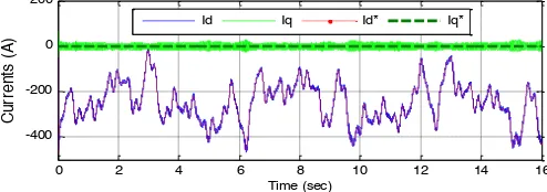
Based on Eq. (15), a variable d-axis reference current is generated as shown in Fig. 14 while q-axis reference current is zero (i.e., zero reactive power), which corresponds to typical wind power production under a fluctuating and gusty wind condition. Due to the motor sign convention used in Fig. 2, power generation from a wind turbine is represented by negative d-axis current values as shown in Fig. 14. Again, the figure shows that the neural network performs very well in tracking the variable reference current in the power converter switching environment.
Fig. 14. Performance of neural vector controllers under a variable reference current condition in power converter switching environment (Ts=1ms)
D. Performance Evaluation under Variable Parameters of GCC System
GCC stability has been one of the main issues to be investigated in conventional vector controls. In general, such studies primarily focus on the GCC performance for either system parameter changes or for unbalanced or distorted ac system conditions. For instance, in [1], a small-signal model is used for a sensitivity study of the GCC under variable system parameter conditions. In [58], a control strategy is developed to improve the GCC performance under variable system conditions. In this paper, the neural control method is investigated for two variable GCC system conditions, namely 1) variation of grid-filter resistance and inductance, and 2) variable PCC voltage.
(a) Actual inductance is 60% above the nominal inductance
(b) Actual inductance is 40% below the nominal inductance
(c) Actual inductance is 50% below the nominal inductance Fig. 15. Performance of conventional standard vector controller (Ts=1ms)
0 1 2 3 4 5 6
-400 -200 0 200 C ur re nt s (A ) Time (sec) Id Iq Id* Iq*
1.95 1.975 2 2.025 2.05
-400 -200 0 200 400 3-ph as e cu rr en ts (A ) Time (sec)
0 1 2 3 4 5 6
-400 -200 0 200 C ur re nt s (A ) Time (sec) Id Iq Id* Iq*
1.95 1.975 2 2.025 2.05
-400 -200 0 200 400 3 -p h a se cu rr e nt s (A ) Time (sec)
0 2 4 6 8 10 12 14 16
-400 -200 0 200 C ur re nt s (A ) Time (sec)
Id Iq Id* Iq*
0 0.5 1 1.5 2 2.5 3 3.5 4
-300 -200 -100 0 100 200 C ur re nt s (A ) Time (sec) Id Iq Id* Iq*
0 0.5 1 1.5 2 2.5 3 3.5 4
-300 -200 -100 0 100 200 C ur re nt s (A ) Time (sec) Id Iq Id* Iq*
0 0.5 1 1.5 2 2.5 3 3.5 4
[image:9.612.48.560.356.726.2]It was found that the neural network controller is mainly affected by variation of the grid-filter inductance but not the resistance. Figure 15 shows how the neural vector controller is affected as the grid-filter inductance deviates from its nominal value used in training the network. In general, if the actual inductance is smaller than the nominal value, the performance of the neural controlled GCC deteriorates (Figs. 15b and 15c). If the actual inductance is larger than the nominal value, the performance of the controller is almost not affected (Fig. 15a). However, as the actual inductance is higher than the nominal inductance, it is easier for the GCC to get into the PWM saturation as explained in [22, 23], particularly for generating reactive power conditions. The study shows that when the actual inductance is over 50% below the nominal value, the impact becomes significant and high distortion and unbalance are found in the grid current (Fig. 15c). A comparison study also demonstrates that the neural controller is much more stable and that it performed better than both conventional standard and DCC vector control methods under the variable grid-filter inductance conditions.
Regarding the variation of the GCC voltage, a special technique is employed in this paper to prevent the neural controller from being affected by the GCC voltage variation. Assume that the nominal and disturbance components of the PCC dq voltage are
v
r
dq n_ andv
r
dq dis_,
respectively. Then, Eq. (6) can be rewritten as(
1 _ _)
dq dq dq dq n dq dis f d
i i v v v L
dt =− ⋅ −Fc −⎡⎣ + ⎤⎦
r r r r r
(16)
where Fc is the continuous system matrix. Since the training of the neural network in Section IV does not consider PCC voltage disturbance, the neural controller will be unable to track the reference demand or lose stability if a high voltage disturbance appears on the PCC bus. One way to overcome the disturbance impact is to introduce d- and q-aixs disturbance voltage terms to the network inputs. However, this makes the training more difficult and the improvement is not evident or worse. Instead of using the disturbance voltage as network inputs, this paper introduces the disturbance voltage to the output of a well trained action network, with the intention of
neutralizing the disturbance. This makes the final control voltage applied to the system become
( )
(
( )
)
1 , _
dq PWM dq dq dis PWM
vr k =k ⋅⎡⎣A ir k wr +vr k ⎤⎦ (17)
where
v
r
dq=
v
r
dq n_+
v
r
dq dis_ is the actual PCC voltage. With the introduction of the disturbance voltage to the output of the action network, the neural network vector control structure, different from Fig. 7, is shown by Fig. 16. The performance evaluation demonstrates that this strategy is very effective to maintain neural network performance under distorted PCC voltage conditions.(a) PCC bus voltage in per unit
(b) dq grid current
[image:10.612.73.545.50.223.2](c) Three-phase grid current
Fig. 17. Performance of neural vector controllers for short-circuit ride through
Figure 17 presents how the neural controller performs under variable PCC voltage caused by a fault. The fault starts at 1s and is cleared at 3s, which causes a voltage drop on the
0 0.5 1 1.5 2 2.5 3 3.5 4
0 0.2 0.4 0.6 0.8 1
PC
C
v
ol
ta
ge
(
p.
u.
)
Time (sec)
0 0.5 1 1.5 2 2.5 3 3.5 4
-300 -200 -100 0 100 200
C
ur
re
nt
s
(A
)
Time (sec) Id
Iq Id* Iq*
2.95 2.975 3 3.025 3.05 -300
-200 -100 0 100 200 300
3-ph
as
e
cu
rr
en
ts
(A
)
Time (sec)
PWM
3/2
3-phase supply 2/3
-
+ v
* a1,b1,c1
vα,β
v*α1
v*
β1
i* d
Vdc
e
j
e
θ-
+ i*q
3/2
iα,β ia,b,c
e j
e
θ idiq
va1,b1,c1 or vd1,q1
∫
∫
Voltage angle calculation
Fig. 16. GCC neural vector control structure when considering voltage disturbance impact. Vd_n and Vq_nare the d and q components of the nominal GCC voltage. In the PCC voltage oriented frame Vq_n=0V and therefore Vq_n is not listed in the figure. kPWMis the gain of the GCC and equals to Vdc/2.
ia,b,c or id,q θe
+
+
+
+
v* d1
v* q1
+
- Vd_n
e
j
e
θvd
vq 1/kPWM
1/kPWM
[image:10.612.311.563.392.686.2]Fig. 19. Neural vector controller in nested-loop control condition
PCC bus during this time period (Fig. 17a) depending on the fault current levels. As it can be seen from Fig. 17b, the neural
vector controller can still effectively regulate the dq current even under a voltage drop of more than 80% at the PCC caused by a fault, demonstrating strong short-circuit
ride-through capability of the neural controller. For many other cases, the neural vector controller demonstrates excellent performance from various aspects. At the start and end of the fault, there is a high peak in the dq current. However, it is necessary to point out that this peak does not mean a high grid current but represents a rapid transition from the previous three-phase current state to a new one (Fig. 17c).
VI. EVALUATION OF NEURAL VECTOR CONTROLLER IN
NESTED-LOOP CONTROL CONDITION
In many renewable and microgrid applications, the GCC control has a nested-loop structure consisting of a faster inner current loop and a slower outer control loop that generates d- and q-axis current references, id* and iq*, to the current loop
[image:11.612.311.560.436.716.2]controller [7, 22]. Figure 18 shows the neural network in the nested-loop control condition, in which the d-axis loop is used for dc-link voltage control and q-axis loop is used for reactive power or grid voltage support control [22, 23]. The error signal between measured and reference dc voltage generates a d-axis current reference to the neural network through a PI controller while the error signal between actual and desired reactive power generates a q-axis current reference. Figure 19 shows the schematics of the neural vector controller in a ac/dc/ac converter structure, which is the typical situation for grid integration of distributed energy resources as shown in Fig. 1. In Fig. 19, the left side represents the grid and the right side represents a renewable energy source (RES) such as a wind turbine. The power transfers from the RES through the dc-link capacitor and the GCC to the grid.
Figure 20 shows the performance of the neural control approach in the nested-loop structure. Before t=4s, the RES generates an active power of 100kW while the GCC reactive power reference is 100kVar, i.e., the GCC should absorb
reactive power from the grid. The initial dc-link voltage is 1200V. Although no synchronization control is employed at the start of the system, both the dc-link voltage and the GCC reactive power are adjusted around the reference values quickly and have very small oscillations by using the neural network control. At t=4s, the active power generated by the RES changes to 200kW, which causes more active power delivered to the grid through the dc-link and the GCC. The reactive power reference is unchanged. Therefore, the dc-link voltage increases. But, with the neural network vector control, the dc-link voltage are quickly regulated around the reference value. At t=8s, the reactive power reference changes from 100kVar to -25kVar, i.e., the GCC should generate reactive power to the grid. At t=12s, the reactive power reference changes from -25kVar to 50kVar, i.e., a condition of absorbing reactive power. In general, for all the reference changes, the neural network controller demonstrates very good performance to meet the nested-loop control requirements.
a) dc link voltage
b) Instantaneous active/reactive power waveforms
c) Grid three-phase current waveforms
Fig. 20. Performance of neural controller in nested-loop control condition
0 2 4 6 8 10 12 14 16
1000 1200 1400 1600 1800
dc
-li
nk
vo
lta
ge
(
V
)
Time (s)
0 2 4 6 8 10 12 14 16
-300 -200 -100 0 100 200
P
ow
er
(
kW
/kV
ar
)
Time (s)
7.95 7.96 7.97 7.98 7.99 8 8.01 8.02 8.03 8.04 8.058.05 -400
-200 0 200 400
ab
c
cu
rr
en
ts
(A
)
Time (s)
-
+ i*d
-
+ i*
q
id
iq
∫
∫
Fig. 18. Nested-loop GCC neural vector control structure PI
V* dc
Vdc
+
-PI V*
bus
-+
Vbus
Reactive power Active
[image:11.612.50.300.580.679.2]VII. CONCLUSIONS
Three-phase grid-connected rectifier/inverters are used widely in renewable, microgrid and electric power system applications. This paper has analyzed the limitations associated with conventional vector control methods for the grid-connected converters. Then, a neural-network based vector control method was developed. The paper described how the vector controller was developed based on a dynamic-programming technique and trained via a backpropagation through time algorithm.
The performance evaluation demonstrated that the neural controller can track the reference d- and q-axis currents effectively even for highly random fluctuating reference currents. Compared to standard vector control methods and direct-current vector control techniques, the neural vector control approach produces the fastest response time, low overshoot, and, in general, the best performance.
To improve neural controller performance and stability under disturbance conditions, we used additional strategies. These include adding integrals of error signals to the network inputs and introducing grid disturbance voltage to the outputs of a well-trained network rather than to the inputs of the network. We have proved that these strategies are effective. In both power converter switching environments and nested-loop control conditions, the neural network vector controller demonstrates strong capability in tracking reference command while maintaining a high power quality. Under a fault in the grid system, the neural controller exhibits a strong short-circuit ride-through capability.
For future work, we plan to purchase equipment and develop hardware experiment system for a laboratory setup as shown by Fig. 19. We believe that the successful hardware experiment would accelerate the commercialization of the proposed neural network vector control technology in power and energy industry.
VIII. ACKNOWLEDGEMENT
The authors would like to thank the reviewers for their helpful comments which contributed to an improved paper.
IX. REFERENCE
[1] E. Figueres, G. Garcera, J. Sandia, F. Gonzalez-Espin, and J.C. Rubio, “Sensitivity Study of the Dynamics of Three-Phase Photovoltaic Inverters With an LCL Grid Filter,” IEEE Trans. on Ind. Electron., vol. 56, no. 3, pp. 706-717, 2009.
[2] C. Wang, and M.H. Nehrir, “Short-Time Overloading Capability and Distributed Generation Applications of Solid Oxide Fuel Cells,” IEEE
Trans. on Energy Convers., vol. 22, no. 4, pp. 898-906, 2007.
[3] A. Luo, C. Tang, Z. Shuai, J. Tang, X. Xu, and D. Chen, “Fuzzy-PI-Based Direct-Output-Voltage Control Strategy for the STATCOM Used in Utility Distribution Systems,” IEEE Trans. on Ind. Electron., vol. 56, no. 7, pp. 2401-2411, July 2009.
[4] J.M. Carrasco, L.G. Franquelo, J.T. Bialasiewicz, E. Galván, R.C.P. Guisado, Ma.Á.M. Prats, J.I. León, and N. Moreno-Alfonso, “Power-Electronic Systems for the Grid Integration of Renewable Energy Sources: A Survey,” IEEE Trans. on Ind. Electron., vol. 53, no. 4, 2006.
[5] L. Xu, and Y. Wang, “Dynamic Modeling and Control of DFIG Based Wind Turbines under Unbalanced Network Conditions”, IEEE Trans. on Power Syst., vol. 22, no. 1, pp. 314-323, 2007.
[6] A. Mullane, G. Lightbody, and R. Yacamini, “Wind-Turbine Fault Ride-Through Enhancement,” IEEE Trans. on Power Syst., vol. 20, no. 4, pp. 1929-1937, 2005.
[7] R. Pena, J.C. Clare, and G.M. Asher, “Doubly fed induction generator using back-to-back PWM converters and its application to variable speed wind-energy generation,” IEE Proc. Electr. Power Appl., vol. 143, no 3, pp. 231-241, 1996.
[8] B.C. Rabelo, W. Hofmann, J.L. Silva, R.G. Oliveira, and S.R. Silva, “Reactive Power Control Design in Doubly Fed Induction Generators for Wind Turbines,” IEEE Trans. on Ind. Electron., vol. 56, no. 10, pp. 4154-4162, 2009.
[9] S. Li and T.A. Haskew, “Transient and Steady-State Simulation of Decoupled d-q Vector Control in PWM Converter of Variable Speed Wind Turbines,” Proc. 33rd Annual Conf. of IEEE Ind. Electron.
(IECON 2007), Taipei, Taiwan, Nov. 5-8, 2007.
[10] S. Li and T.A. Haskew, “Analysis of Decoupled d-q Vector Control in DFIG Back-to-Back PWM Converter,” Proc. 2007 IEEE Power
Engineering Society General Meeting, Tampa FL, June 24-28, 2007.
[11] P. Fischer, “Modeling and control of a line-commutated HVDC transmission system interacting with a VSC STATCOM,” Ph.D.
dissertation, School Electr. Eng., Royal Inst. Technol. Stockholm,
Sweden, 2007.
[12] U.I. Dayaratne, S.B. Tennakoon, N.Y.A. Shammas, and J.S. Knight, "Investigation of variable DC link voltage operation of a PMSG based wind turbine with fully rated converters at steady state," Proc. 14th
European Conf. on Power Electron. and Appl., Birmingham, UK, Aug.
30 - Sept. 1 2011
[13] J. Rocabert, G.M.S. Azevedo, A. Luna, J.M. Guerrero, J.I. Candela, and P. Rodr´ıguez, “Intelligent Connection Agent for Three-Phase Grid-Connected Microgrids,” IEEE Trans. on Power Electron., vol. 26, no. 10, pp. 2993-3005, 2011.
[14] D. Jovcic, L.A. Lamont, and L. Xu, “VSC transmission model for analytical studies,” Proc. 2003 IEEE Power Engineering. Society
General Meeting, Toronto, Canada, 2003.
[15] M. Durrant, H. Werner, and K. Abbott, “Model of a VSC HVDC terminal attached to a weak ac system,” Proc. IEEE Conf. Control
Appl., Istanbul, Turkey, pp. 178–182, 2003.
[16] L. Harnefors, M. Bongiornos, and S. Lundberg, “Input-admittance calculation and shaping for controlled voltage-source converters,”
IEEE Trans. Ind. Electron., vol. 54, no. 6, pp. 3323–3334, 2007.
[17] I. Codd, “Windfarm Power Quality Monitoring and Output Comparison with EN50160”, Proc. 4th Int. Workshop on Large-scale Integration of Wind Power and Transmission Networks for Offshore
Wind Farm, Sweden, Oct. 20-21, 2003.
[18] B.I. Nass, T.M. Undeland, and T. Gjengedal, “Methods for Reduction of Voltage Unbalance in Weak Grids Connected to Wind Plants”, Proc. IEEE Workshop on Wind Power and the Impacts on Power
Systems, Oslo, June 2002.
[19] A. Timbus, R. Teodorescu, F. Blaabjerg and M. Liserre, “Synchronization Methods for Three Phase Distributed Power Generation Systems - An Overview and Evaluation,” Proc.36th IEEE Power Electronics Specialists Conference, Recife, Brazil, pp. 2474 - 2481, June 12-16 2005.
[20] L. Zhang, “Modeling and control of VSC-HVDC links connected to weak AC systems,” Ph.D. dissertation, School Electr. Eng. Royal Instit. Technol., Stockholm, Sweden, 2010.
[21] L. Zhang, L. Harnefors, and H.P. Nee, “Power-synchronization control of grid-connected voltage-source converters,” IEEE Trans. Power Syst., vol. 25, no. 2, pp. 809–820, 2010.
[22] S. Li, T.A. Haskew, Y. Hong, and L. Xu, “Direct-Current Vector Control of Three-Phase Grid-Connected Rectifier-Inverter,” Electric
Power System Research, Vol. 81, Issue 2, pp. 357-366, 2011.
[23] S. Li, T.A. Haskew, and L. Xu, “Control of HVDC Light Systems using Conventional and Direct-Current Vector Control Approaches,”
IEEE Trans. on Power Electron., vol. 25, no. 12, pp. 3106-3118, 2010.
[24] T. Noguchi, H. Tomiki, S. Kondo, and I. Takahashi, “Direct power control of PWM converter without power-source voltage sensors,”
IEEE Trans. Ind. Appl., vol. 34, no. 3, pp. 473–479, 1998.