Multi-perspective analysis of mobile phone call data records: A visual analytics approach

City, University of London Institutional Repository

Citation

:

mobile phone call data records: A visual analytics approach. Paper presented at the Multi-perspective Analysis of Mobile Phone Call Data Records: a Visual Analytics Approach.

This is the accepted version of the paper.

This version of the publication may differ from the final published

version.

Permanent repository link:

Link to published version

:

Copyright and reuse:

City Research Online aims to make research

outputs of City, University of London available to a wider audience.

Copyright and Moral Rights remain with the author(s) and/or copyright

holders. URLs from City Research Online may be freely distributed and

linked to.

City Research Online: http://openaccess.city.ac.uk/ [email protected]

Multi-perspective Analysis of Mobile Phone Call Data

Records: a Visual Analytics Approach

Gennady Andrienko1,2_{, Natalia Andrienko}1,2_{, Georg Fuchs}1

1 _{Fraunhofer Institute IAIS, Schloss Birlinghoven, 53757 Sankt Augustin, Germany} 2 _{City University London, Northampton Square, London EC1V 0HB, UK}

{Gennady.Andrienko, Natalia.Andrienko, Georg.Fuchs}@iais.fraunhofer.de

Abstract. Analysis of human mobility is currently a hot research topic in data mining, geographic information science and visual analytics. While a wide variety of methods and tools are available, it is still hard to find recommendations for considering a data set systematically from multiple perspectives. To fill this gap, we demonstrate a workflow of a comprehensive analysis of a publicly available data set about mobile phone calls of a large population over a long time period. We pay special attention to the evaluation of data properties. We outline potential applications of the proposed methods.

Keywords: visual analytics, mobility data, call data records.

1 Introduction

Nowadays, huge amounts of movement data describing changes of spatial positions of discrete mobile objects are collected by means of contemporary tracking technologies such as GPS, RFID, and positions within mobile phone call records. Extensive research on trajectory analysis has been conducted in knowledge discovery in databases [1], spatial computing [2], and moving object databases [3]. Automatically collected movement data are semantically poor as they basically consist of object identifiers, coordinates in space, and time stamps. Despite that, valuable information about the objects and their movement behavior, as well as about the space and time in which they move can be gained even from such basic movement data by means of analysis [4].

Movement can be viewed from multiple perspectives: as consisting of continuous paths in space and time [5], also called trajectories, or as a composition of various spatial events [6]. Movement data can be aggregated in space, enabling identification of interesting places and studying their activity characteristics, and by time intervals, enabling similarity analysis of situations comprising different time intervals as well as detection of extraordinary events.

For the most comprehensive analysis of movement data, the analyst would look at the data from all perspectives: mover-oriented, event-oriented, space-oriented, and time-oriented. However, data properties often limit possible directions of analysis.

properties of the data that restrict potentially applicable movement data analysis methods (Section 2). A first analysis step is to study spatio-temporal patterns of calling activities at multiple resolutions of time. To this end we apply spatio-temporal aggregations by antennas, counting number of calls per day (Section 3) and per hour (Section 4). To further identify different kinds of activity neighborhoods and to study their spatial distribution we then characterize antennas by feature vectors of hourly activities within a week and cluster them by similarity of the feature vectors (Section 5). In order to identify peak events – i.e., time intervals during which extraordinarily large number of people made calls in one location simultaneously - we compare time series comprising counts of distinct phone users per time interval and antenna (Section 6). This procedure allows us to identify large-scale events that, possibly, happened in the country. We use trajectories of mobile phone subscribers for reconstructing flows between major towns and between activity regions of the country (Section 7). Finally, we make an attempt at semantic interpretation of individuals’ personal places, such as home and work locations, based on these user trajectories (Section 8). We conclude this paper with an outline of a general procedure of data analysis from multiple perspectives (Section 9) and a short discussion on the results and possible directions for further work.

2 Evaluating Data Properties

In analyzing movement data, it is important to take into account the following properties [14]:

• Temporal properties:

o temporal resolution: the lengths of the time intervals between the position measurements;

o temporal regularity: whether the length of the time intervals between the measurements is constant or variable;

o temporal coverage: whether the measurements were made during the whole time span of the data or in a sample of time units, or there were intentional or unintentional breaks in the measurements;

o time cycles coverage: whether all positions of relevant time cycles (daily, weekly, seasonal, etc.) are sufficiently represented in the data, or the data refer only to subsets of the positions (e.g., only to work days or only to daytime), or there is a bias towards some positions.

• Spatial properties:

o spatial resolution: the minimal change of position of an object that can be reflected in the data;

o spatial precision: whether the positions are defined as points (by exact coordinates) or as locations having spatial extents (e.g. areas). For example, the position of a mobile phone call is typically a cell in a mobile phone network;

studied territory (in terms of the spatial extent, uniformity, and density)?

• Mover set properties:

o number of movers: a single mover, a small number of movers, a large number of movers;

o population coverage: whether there are data about all movers of interest for a given territory and time period or only for a sample of the movers;

o representativeness: whether the sample of movers is representative, i.e., has the same distribution of properties as in the whole population, or biased towards individuals with particular properties. • Data collection properties:

o position exactness: How exactly could the positions be determined? Thus, a movement sensor may detect an object within its range but may not be able to determine the exact coordinates of the object. In this case, the position of the sensor will represent the position of the object in the data;

o positioning accuracy, or how much error may be in the measurements;

o missing positions: in some circumstances, object positions cannot be determined, which leads to gaps in the data;

o meanings of the position absence: whether absence of positions corresponds to stops, or to conditions when measurements were impossible, or to device failure, or to private information that has been removed.

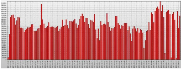
The provided data set [7] comprises a total of 55,319,911 CDRs distributed over ten individual chunks of between 4.8 and 6.5 million records, each corresponding to a set of two-week time intervals. Of these, 47,190,414 CDRs are associated with one of the 1,214 antennas and thus be referenced by the corresponding antenna’s geographic coordinates. CDR temporal references are given with minute accuracy (i.e., seconds were suppressed) ranging from December 5, 2011 till April 22, 2012. Aggregation of geo-referenced calls by days (Figure 1) shows that some days (e.g. March 24, 2012) have much less number of calls than neighboring days. This observation suggests that quite many call activities are missing in the database, especially in April 2012. In addition, 8,129,497 calls refer to unknown antennas (id=-1), with maximal count 166,621 calls on April 1, 2012. Because these CDRs could not be geo-located and thus not related to other calls originating from the same location they were ignored during data import.

The figure also suggests obvious call peak patterns at New Year, Easter, and, to some extent, at Christmas 2011. Other peaks correspond to public holidays like The Day after the Prophet's Birthday (Sunday, February 5, 2012) and Post African Cup of Nations Recovery (Monday, February 13,2012)1.

1 _{Public holidays in Ivory Coast in 2012:}

Fig. 1. Daily counts of calls.

Fig. 2. Space-Time Cube displaying the full 20-week data set of CDRs integrated into trajectories (sequence of calls with the same user id) with time increasing from bottom to top of the cube. Besides expected daily cycles e.g. in the area of Abidjan one can spot missing days (near the top), and very clearly the distinct pattern of bi-weekly “false trip” movement caused by re-assigning user IDs to different mobile phone users in other parts of the country between data chunks.

Wikipedia2 suggests that religion in Ivory Coast remains very heterogeneous, with Islam (almost all Sunni Muslims) and Christianity (mostly Roman Catholic) being the major religions. Muslims dominate the north, while Christians dominate the south. Unfortunately, the amount of data available for the northern part of the country does not allow comparison of patterns in respect to religious holidays.

A considerable constraint in terms of mobility pattern analysis and semantic interpretation (Sections 7 and 8, respectively) arises from the anonymization procedure applied to the data [7]. Each of the 10 data chunks is a subset of 50,000 distinct mobile phone subscribers tracked over 2 weeks. User IDs associated with each CDR are obviously not real, traceable customer IDs but rather consecutive integer numbers. And while a given user ID is unique with respect to one data chunk, integers are reused (i.e., the counter was reset) between different chunks. This means that it is not possible to analyze movement patterns or flows over periods exceeding two weeks, or generally cover time intervals distributed over multiple chunks (compare Figure 2).

Moreover, a check for repeated combinations of user ID and time stamp produced 5,225,989 pairs that occurred 12,861,168 times in the database. The duplicates have been removed. This operation thus reduced the number of geo-referenced CDRs in the database by about 25%.

3 Assessing daily aggregates for antennas

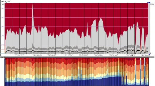
We have aggregated the remaining CDRs by antennas and days, producing daily time series of calls for each of the 1,214 antennas. Figure 3 presents an overview of their statistical properties. The upper part of the image shows the call counts’ running average line (in bold) and dynamics by deciles (grey bands, min = 0, 10%, 20%, …, 90%, max = 5584) over time. Vertical lines correspond to weeks. The lower part of the image uses segmented bars to represent distribution of antennas categorized by their daily call counts. The darkest blue denotes absence of any calls at those antennas; blue colors correspond to intervals from 1 to 50 calls per day, yellow represents 50 to 100 calls, orange and reds – more than 100 calls.

Fig. 3. Top: dynamics of deciles of counts of call per antenna distributions. Bottom: daily proportions of antennas with N calls in intervals of 0 (darkest blue), 1..10, 10..50, 50..100 (yellow), 100..200, 200..500, 500..1000, and more than 1000 (darkest red) per day. Note that in the upper image, corresponding interval boundaries are indicated in the scale to the left.

 Too few data records on Dec 5, 2011 even though CDR time stamps for that day cover the entire 24h period.

 Gradual increase of counts of antennas without activity (0 calls per day) from Dec 6, 2011 till March 27, 2012.

 Several days with missing data on many antennas (March 29, April 1, April 10, April 15, April 19).

 Absence of typical weekly patterns with different amounts of calls at working days and weekends.

Fig.4. Mosaic (segmented) diagrams show counts of calls for all antennas in the whole country. Counts are represented by colored segments ranging from blue (0 calls) through yellow (50..100 calls) to red (more than 1,000 calls). Diagram rows correspond to weeks (top to bottom – from week 1 to week 20) and columns to days of week (left to right: from Monday to Sunday)

Monday to Sunday, from left to right) and rows correspond to weeks (from 1 to 20, from top to bottom). Figure 4 shows the entire country, Figure 5 a close-up of the region of the towns Abidjan and Abobo. The large consecutive sections of dark blue colors in many diagrams suggest that the data contain systematically missing portions. In particular, data are completely unavailable 12-14 weeks for many antennas in the northern part of the country, and for more than 16 weeks in the southern part of Abidjan.

Fig. 5. Close-up view of the region of the towns Abidjan and Abobo. The mosaic diagrams are encoded in the same way as in Figure 4 and use the same color coding.

application of analysis methods developed primarily for European countries is not valid.

One more complexity of the data is caused by the data sampling and anonymization procedures [7]. For each two-week period, a subset of 50,000 customers has been selected. It is not guaranteed that the subsets represent population samples with similar demographic and economical characteristics. Indeed, clustering days by feature vectors comprising counts of calls at each antenna, followed by assigning colors to clusters by similarity [8] clearly demonstrates the dissimilarity of patterns in consecutive two-weeks periods (Figure 6). Additionally, this display also does not give any evidence of differences between week days and weekends.

Fig. 6. Similarity of situations during 7 days x20 weeks, represented by assigning colors to segments of the diagram according to the cluster the corresponding day belongs to.

4 Analyzing hourly aggregate patterns for antennas

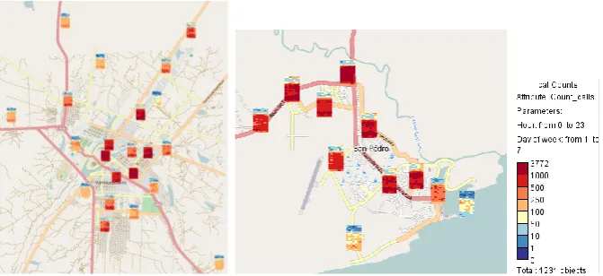
Taking into account the properties of the data, we decided to aggregate calls by antennas for hours of day and days of week, irrespectively of calendar dates. Figure 7 shows mosaic diagram maps for two locations, the country’s capital (Yamoussoukro) and a port town (San Pedro). Like in Figures 4 and 5, the diagrams consist of segments representing call counts by colors, from dark blue (no calls) through yellow (50-100 calls per hour) to red. The segments of each diagram are arranged by days of week (Monday to Sunday from left to right) and by hours of day (from 0:00 on top to 23:00 at bottom).

Fig. 7. Mosaic diagrams show hourly absolute counts of calls for 7 days of week (by columns, from Monday to Sunday) and 24 hours of day (from 0:00 to 23:00) in Yamoussoukro and San Pedro.

Fig. 8. Similarly to Figure 7, mosaic diagrams show hourly show counts of calls for 7 days of week (by columns, from Monday to Sunday) and 24 hours of day (from 0:00 to 23:00) normalized by average count per antenna in Yamoussoukro and San Pedro.

5 Clustering antennas by similarity of hourly aggregate patterns

Visual inspection and comparison of mosaic diagrams has limited applicability. We can perform it for selected cities and regions, but can’t apply systematically for the whole country. Instead, we can apply clustering of antennas according to mean-normalized hourly activity profiles over week. We’ve used k-Means and varied the desired number of clusters from 5 to 15, the most interpretable results have been obtained with N=7. Lower number of clusters mixes several behaviors, while large counts extract small clusters with too specific behaviors.

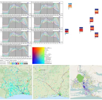
The results are presented in Figure 9. Seven time graphs show profiles of the 7 clusters for 7 days of week. Centroids of the clusters have been projected onto the 2d plane by Sammons mapping [9] (middle left). Following the ideas of [10], colors have been assigned to the clusters according to these 2D positions, thus reflecting relative cluster similarities. The representative feature vector of the cluster centroids are presented by mosaic diagrams (middle right, days of week in columns, hours of day in rows, similarly to Figures 7 and 8), with their placement again corresponding to the respective centroid’s Sammons projection. Using these visualizations, we can suggest some interpretations to the clusters:

Cluster 1:High calling activity in the evenings, irrespective of the day of week. Such a profile is typical for residential districts with a high proportion of employed population.

Cluster 2:Uniform calling activity during the day, with some increase in the morning on Monday, Wednesday, Friday and Saturday.

Cluster 3:High calling activity in the evenings, medium activity in mornings, and decreased activity in the middle of the day (except Sundays)

Cluster 4:High calling activity during working hours (except Sundays), with extremes in mornings. Such a profile is typical for business districts. Cluster 5:Very low calling activity, with only small differences between day and

night. This is quite typical for unpopulated areas and for antennas masked (in terms of call handling) by neighboring antennas.

Cluster 6:Similar to cluster 3, however with a less prominent evening pattern but more prominent morning pattern, and increased activity on Saturdays and Sundays.

Cluster 7:Similar to clusters 3 and 6, but with decreased activity on Sundays.

Our experience of analyzing mobile phone usage data in different countries suggests that cluster 1 corresponds to residential districts with high proportion of regularly employed population, in other words, people having fixed out-of-home work schedules, and that cluster 4 represents business districts. We guess that cluster 2 either represents regions with a mix of residential and business land use, or businesses with irregular schedules. Major transportation corridors (main roads, railways) can be characterized by similar temporal patterns, too. Clusters 3, 6 and 7 may represent mostly residential areas with partly employed population, or population with flexible work schedule.

Abidjan, respectively. We can observe that our possible interpretations correspond to geographical patterns.

Fig. 9. Normalized temporal signatures of antennas are used for defining 7 clusters by k-Means. Time graphs in the upper panel show profiles of these clusters during 7 days of week. Colors are assigned to the clusters according to positions of cluster centroids in Sammons mapping (middle). Representative activity profiles for the clusters are shown by 2D mosaic diagrams in the yop-right. The maps at the bottom show spatial distributions of the clusters for the whole country (left), south-west part (center) and the region around Abidjan (right).

6 Peak detection from hourly time series at antenna level

portions, therefore limiting time intervals eligible for such analysis in this particular data set due to the inability to distinguish users between data chunks.

We focus our further analysis on trajectories (sequences of positions) of different users during last two weeks of the data set. This is the only period that contains rather complete geographic coverage, see Section 3 for details. For each distinct antenna we have computed hourly counts of distinct user IDs active at this antenna. These counts roughly represent the presence of people in antenna cells. If a person made several calls from the same antenna, we assume that he did not move away between the calls. It should be noted that this assumption may be incorrect in some cases, in that people may transition out of an antenna’s cell and back without making a call at another antenna in the meantime.

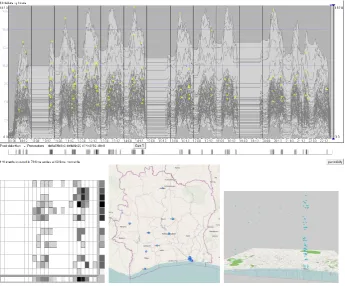
Fig. 10. The time graph at the top shows time series of counts of mobile phone users grouped by antennas, at 1 hour resolution. Peaks with magnitude of at least 20 users over 3 hour intervals are marked by yellow crosses. Counts of peaks are shown in 2d periodic event bar at the left. Positions of peak events are shown on the map of the country in the bottom-center map and in the space-time cube at bottom-right.

presence magnitudes exceeding 20 distinct peoples over a sliding, 3 hours time window [11]. The appropriate parameters for magnitude threshold and time window width have been defined using a sensitivity analysis procedure as suggested by [12]. In particular, the time graph in Figure 10 (top) only shows lines for those antennas that exhibit at least one such peak event. The horizontal event bar immediately below the time graph shows the counts of events over time. The 2D periodic event bar in Figure 10 (bottom left) shows counts of peak events per 24 hours of day (columns) and 14 days of two weeks (rows). The map (bottom-center) and space-time cube (bottom-right) show spatial and spatio-temporal distributions of peak events.

We can observe that peak events are frequent in the middle of the day and early in the evening. There are only few exceptions. Thus, several peak events happened during the 15:00 – 16:00h interval on Monday and Fridays of the 1st _{week, and late in}

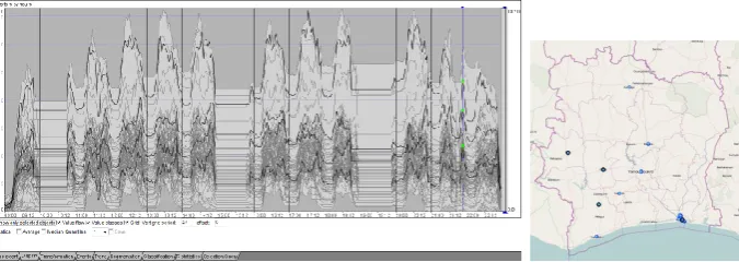
the evening of Saturday of the 2nd _{week. By clicking the corresponding segment of the}

periodic event bar, we select the corresponding antennas and time series (see Figure 11). We can see that these peaks happened in 4 different towns in different parts of the country. The time series profiles for those regions indicate that these peaks are rather unusual. We guess that some kind of connected public events happened simultaneously in these regions.

Fig. 11. Peaks that happened at 21:00 on the 2nd _{week’s Saturday and their containing time}

series are highlighted in the time graph (left). Simultaneously, their positions are marked on the map (right).

It is interesting to relate the magnitude of peaks with the maximal values of the time series. We found two extreme cases of time series with peaks of more than 20 people contained in time series with maximum (peak) values of about 40 but average daily values of only about 10..15 people (Figure 12). Both events happened in Abidjan. Probably, some local events happened at about 10:00 on Monday and at 21:00 of Thursday in these locations.

Fig. 12. Peaks on Monday morning (yellow cross) and Thursday evening (green cross) are shown on top of two time series with otherwise usually low presence of calling activities. Both peaks have happened in Abidjan.

Fig. 13. Flows between regions that correspond to peaks in people presence.

7 Analysis of flows

Figure 14 (left) shows the original trajectories rendered with high level of transparency (about 99%). This representation gives us a hint about major flows, but does not allow quantifying them. Figure 14 (right) shows the flows between aggregated regions as well as the accumulated counts of distinct users recorded in each region during the two-week period.

We can observe the consistency between the flow maps in Figures 13 and 14, respectively. However, the latter map uncovers more structural details. In particular, we can see a branch connecting Abidjan with the mid-eastern region of the country. There are only relatively few direct connections between Abidjan and Yamoussoukro, and fewer still between these two and towns in the northern part of the country. This indicates that despite the existences of several local airports, people mostly use ground transportation and make phone calls / send SMS during their lengthy trips. By contrast, air travel typically manifests itself as long-distance flows since the mobile phone is switched of or out of range during flight with no calls at intermediate antennas.

Further analysis (omitted here for space / time constraints) could allow us to identify temporal patterns of flows and assess usual travel times between different locations. We could also find frequent sequences of visited regions and assess the dynamics of such trips.

Fig. 14. All trajectories during last two weeks drawn as accumulation of semi-transparent lines (left). Trajectories are summarized by 28 aggregated regions (Voronoi polygons) of approximately 100km radius. Flows between regions are represented by red arrows with flow magnitudes encoded in the arrow width. Counts of mobile phone owners registered in each area are shown by yellow bars.

8 Semantic analysis of personal places

two weeks of the data period and with bounding rectangle diagonals exceeding 5km. The total number of call records in this sample is 133,029. First, we have identified stops as sequences of consecutive calls that occurred within 30 minutes and a rectangular region of less than 500m diagonal. Using these parameters extracted 7,149 stops. The stops have then been clustered by means of the density-based clustering method Optics [155], separately for each trajectory. Parameters have been chosen to group points having at least 5 neighbors within 500m distance. Noise points not grouped into any cluster (1,300 points in total, or about 19% of the set) have been excluded from subsequent analysis as they are assumed to represent infrequently visited locations. For each cluster the counts of calls have been aggregated for every hour of the day. This resulted in time series comprised of 24 one-hour intervals assigned to each cluster.

Fig. 15. Individual locations of repeated activities are shown by 500m buffer polygons for subscriber #548709. Hourly temporal signatures (according to hours of day) are shown by time flow diagrams. Spatio-temporal positions of calls are shown in the space-time cube. Red dots represent home-based calls, blue dots correspond to the person’s work place, and prurple to the primary location of her evening activities. Gray dots in the space-time cube represent irregular activities.

including night times (but less during the day). We interpret this place as the person’s home.

Fig. 16. Locations from other trajectories characterized by temporal profiles similar to that was identified as work in Figure 15.

A better quality of semantic interpretation could be achieved if CDRs included times and positions of both the beginnings and ends of calls. In this case it becomes possible to distinguish stationary calls from calls on move, and to estimate movement speeds during the latter.

By applying the described procedure systematically to all subsets of the data and matching routine activity locations of persons in different subsets, it might further be possible to link partial trajectory corresponding to the same person in different data chunks (see Section 2). However, such re-integration may be harmful in terms of personal privacy [166].

9 A general procedure of analysis

In this section, we attempt to outline a general procedure for analyzing movement data from multiple perspectives. For the most comprehensive analysis of movement data, the analyst would look at the data from all perspectives: mover-oriented, event-oriented, space-event-oriented, and time-oriented. Such an analysis would include the following groups of tasks:

• Mover-oriented tasks dealing with trajectories of movers:

o Characterize trajectories as units in terms of their positions in space and time, shapes, and other overall characteristics.

o Analyze the variation of the positional attributes in space and time.

o Discover and investigate occurrences of various types of relations between the movers and the spatio-temporal context, including other movers.

• Event-oriented tasks dealing with relevant spatial events, in particular, events that have been extracted from trajectories, local presence dynamics, or spatial situations in the process of the analysis:

o Characterize the relevant events in terms of their spatio-temporal positions and thematic attributes.

o Discover and investigate occurrences of various types of relations between the events and the spatio-temporal context, including other events.

• Space-oriented tasks dealing with a set of places of interest (POI) and local dynamics (temporal variations) of presence and flows:

o Define a set of relevant POI.

o Characterize the POI in terms of the local presence dynamics.

o Characterize binary links between the POI in terms of the flow dynamics.

• Time-oriented tasks dealing with a set of time units and respective spatial situations:

o Characterize the time units in terms of the spatial situations.

o Discover and characterize the relations between the time units imposed by movers and/or events, in particular, similarity and change relations.

This list of tasks is not meant to specify any order in which the tasks should be performed. During the process of analysis, tasks of different types intermix; however, they do not intermix fully arbitrarily but follow one another in certain logical sequences.

It is not necessary that all types of tasks are included in an analysis. Only a subset of tasks may be relevant to the analysis goals.

Based on our experience and the existing dependencies between the analytical methods in terms of their inputs and outputs, we can suggest a number of possible rational sequences of tasks in movement analysis. These task sequences are presented in Figure 17 in the form of flow chart. The tasks are represented by brief descriptions preceded by characters M, E, S, or T, which denote the possible task foci: Movers, Events, Space, and Time.

Although the graph specifying the possible task sequences has a single root node, it does not mean that any analysis must begin with the task “Analyze trajectories as units” represented by this node. For a particular application, the characteristics of trajectories as units may be of no interest but analysts may be interested first of all in the positional attributes or in relations of movers to the context or in aggregated movement characteristics over a given territory. Furthermore, the analysis may initially focus on spatial events, in particular, when the movement data are originally available in the form of spatial events rather than trajectories, as, for example, data from Flickr or Twitter or data about mobile phone use. In the flow chart, the nodes where the analysis can start are marked by grey background.

It is also not necessary that the analysis ends only when one of the terminal nodes is reached and the respective task fulfilled. The analysis may end in any intermediate node when the application-relevant analysis goals are achieved. The analysis may also continue by switching to another branch. In particular, there are two terminal nodes labelled “M: Analyze trajectories responsible for the discovered relations” (where relations between POI or time units are meant). Here it is assumed that a subset of trajectories is selected for which the analysis is done starting from the root node of the flowchart and following the left branch.

Fig. 17. The flow chart represents possible sequences of tasks in movement analysis.

10 Conclusions

In this paper, we report on analysis results of a medium-size set of call data records referring to antenna positions. The analysis was performed with V-Analytics – a research prototype integrating visual analytics techniques for spatial, temporal and spatio-temporal data that our group develops since the mid-90s [177]. We considered

M: Analyse trajectories as units

M: Analyse positional attributes

M: Analyse relations to context

M: Extract movement events

M: Extract relation events

E: Analyze movement events

E: Analyze relation events

M: Analyze event impact

S: Define POI based on events

E,M: Aggregate events or trajectories by POI and time units

S: Analyse dynamics of events or mover presence in POI

S: Analyse relations between POI

S: Define POI based on trajectories

(space tessellation)

M: Aggregate trajectories by POI and time units

S: Analyse dynamics of presence and flows

T: Analyse spatial situations

S: Analyse temporal and ordering relations

between POI

M: Analyse trajectories responsible for the discovered relations

S: Extract peak/pit events from presence

or flow dynamics

T: Extract peak/pit events from spatial situations

T: Analyse change relations between

time units

M: Analyse trajectories responsible for the discovered relations

E: Analyse peak/pit events

M: Analyze event impact

the data from multiple perspectives, including views on locations of varying resolution, time intervals of different length and hierarchical organization, and trajectories. We detected a number of interesting patterns that could facilitate a variety of applications, including

 Reconstructing demographic information (to replace expensive and difficult to organize census studies)

 Reconstructing patterns of mobility (to enhance transportation studies)

 Identifying places of important activities (for improving land use and infrastructure)

 Identifying events (for improving safety and security)

 Detecting social networks (for marketing purposes)

While in some cases we considered the complete data set, we had to restrict parts of our analysis to the last two weeks of the provided data due to undesirable properties (namely, missing, incomplete or duplicate data records for several key regions for a large portion of the time period). However, most of the applied techniques scale (or can be scaled up conceptually) for much larger data sets. Some kinds of analysis that we planned to perform were simply impossible due to the data fragmentation into chunks with duplicate user IDs. For example, we were not able to build predictive models of people’s presence and mobility [188], as data for longer time periods are needed. We also did not search for interaction patterns between people and did not try to detect social networks.

Limitation caused by data quality could be relaxed by joining the provided data set with data from publicly available sources such as Flickr and Twitter in future work. Textual aggregates of activity records could greatly facilitate understanding and deeper semantic interpretation of the data.

References

1. F.Giannotti, D. Pedreschi (Eds.). Mobility, Data Mining and Privacy - Geographic Knowledge Discovery. Springer, 2008.

2. P.Laube. Progress in movement pattern analysis. In BMI Book (2009), Gottfried B., Aghajan H. K., (Eds.), vol. 3 of Ambient Intelligence and Smart Environments, IOS Press, pp. 43–71.

3. R.H.Güting, M.Schneider. Moving Objects Databases. Morgan Kaufmann, 2005

4. G.Andrienko, N.Andrienko, P.Bak, D.Keim, S.Kisilevich, S.Wrobel. A conceptual framework and taxonomy of techniques for analyzing movement. Journal of Visual Languages and Computing, 2011, 22(3), pp.213-232

5. T.Hägerstrand. What about people in regional science? Papers, Regional Science Association, 24, 1970, pp.7-21.

6. G.Andrienko, N.Andrienko, M.Heurich. An event-based conceptual model for context-aware movement analysis. International Journal Geographical Information Science, 2011, 25(9), pp.1347-1370

8. G.Andrienko, N.Andrienko, P.Bak, S.Bremm, D.Keim, T.von Landesberger, C.Pölitz, T.Schreck. A Framework for Using Self-Organizing Maps to Analyze Spatio-Temporal Patterns, Exemplified by Analysis of Mobile Phone Usage. Journal of Location Based Services, 2010, v.4 (3/4), pp.200-221

9. J.W.Sammon. A nonlinear mapping for data structure analysis. IEEE Transactions on Computers, 1969, v.18, pp.401–409

10. G.Andrienko, N.Andrienko, S.Bremm, T.Schreck, T.von Landesberger, P.Bak, D.Keim. Space-in-Time and Time-in-Space Self-Organizing Maps for Exploring Spatiotemporal Patterns. Computer Graphics Forum, 2010, v.29 (3), pp.913-922

11. G.Andrienko, N.Andrienko, M.Mladenov, M.Mock, C. Pölitz. Discovering Bits of Place Histories from People's Activity Traces. In IEEE Visual Analytics Science and Technology (VAST 2010), Proceedings, IEEE Computer Society Press, pp.59-66

12. G.Andrienko, N.Andrienko, M.Mladenov, M.Mock, C. Pölitz. Identifying Place Histories from Activity Traces with an Eye to Parameter Impact. IEEE Transactions on Visualization and Computer Graphics, 2012, v.18 (5), pp.675-688

13. N.Andrienko, G.Andrienko. Spatial Generalization and Aggregation of Massive Movement Data. IEEE Transactions on Visualization and Computer Graphics, 2011, v.17 (2), pp.205-219

14. G.Andrienko, N.Andrienko, P.Bak, D.Keim, S.Wrobel. Visual Analytics of Movement. Springer, 2013.

15. M.Ester, H.-P.Kriegel, J.Sander, X.Xu. A density-based algorithm for discovering clusters in large spatial databases with noise. Second International Conference on Knowledge Discovery and Data Mining, Portland, Oregon, 1996, pp.226-231

16. G.Andrienko, N.Andrienko. Privacy Issues in Geospatial Visual Analytics. 8th Symposium on Location-Based Services (LBS 2011), Proceedings, Springer, pp.239-246 17. N.Andrienko, G.Andrienko. Visual Analytics of Movement: an Overview of Methods,

Tools, and Procedures. Information Visualization, 2013, v.12(1), pp.3-24