Identification and Estimation of Differentiated Products Models using Market Size and Cost Data

City, University of London Institutional Repository

Citation

: Byrne, D. P., Imai, S., Jain, N., Sarafidis, V. and Hirukawa, M. (2015).

Identification and Estimation of Differentiated Products Models using Market Size and Cost Data (15/05). London, UK: Department of Economics, City University London.

This is the published version of the paper.

This version of the publication may differ from the final published

version.

Permanent repository link:

Link to published version

: 15/05

Copyright and reuse:

City Research Online aims to make research

outputs of City, University of London available to a wider audience.

Copyright and Moral Rights remain with the author(s) and/or copyright

holders. URLs from City Research Online may be freely distributed and

linked to.

Department of Economics

Identification and Estimation of Differentiated Products

Models using Market Size and Cost Data

David P. Byrne

University of Melbourne

Susumu Imai1

University of Technology Sydney and Queen’s University

Neelam Jain

City University London

Vasilis Sarafidis

MonashUniversity

Masayuki Hirukawa

Setsunan University

Department of Economics Discussion Paper Series

No. 15/05

Identification and Estimation of Differentiated

Products Models using Market Size and Cost Data

∗

.

David P. Byrne

Susumu Imai

Neelam Jain

Vasilis Sarafidis

and Masayuki Hirukawa

.

August 8, 2015

Abstract

We propose a new methodology for estimating the demand and cost functions

of differentiated products models when demand and cost data are available. The

method deals with the endogeneity of prices to demand shocks and the endogeneity

of outputs to cost shocks, by using variation in market size that does not need to be

exogenous, and cost data. We establish nonparametric identification, consistency

and asymptotic normality of our estimator. Using Monte-Carlo experiments, we

show our method works well in contexts where instruments are correlated with

de-mand and cost shocks, and where commonly-used instrumental variables estimators

are biased and numerically unstable.

∗_{We are grateful to Herman Bierens, Micheal Keane, Robin Sickles and the seminar participants at the}

University of Melbourne, Monash University, ANU, Latrobe University, UTS, UBC, UNSW, University of Sydney, University of Queensland, City University London and Queen’s for comments.

†_{Dept. of Economics, University of Melbourne,[email protected].}

‡_{Corresponding author, Economics Discipline Group, University of Technology Sydney and Queen’s}

University, e-mail: [email protected].

§_{Department of Economics, City University London, e-mail: [email protected].}

¶_{Department of Econometrics and Business Statistics, Monash University, e-mail: vasilis.sarafidis} @monash.edu.

k_{Department of Economics, Setsunan University, e-mail:}

Keywords: Differentiated Goods Oligopoly, Instruments, Parametric Identifica-tion, Nonparametric IdentificaIdentifica-tion, Cost data.

1

Introduction

In this paper, we develop a new methodology for estimating models of differentiated

products markets. Our approach requires commonly used demand-side data on products’

prices, market shares, observed characteristics and some firm-level cost data. The novelty

of our method is it does not use conventional instrumental variables strategies to deal with

the endogeneity of prices to demand shocks in estimating demand, nor the endogeneity of

outputs to cost shocks in estimating cost functions. Instead, we use variation in market

size (which does not need to be exogenous) and cost data for identification.

The frameworks of interest are the logit and random coefficient logit models of Berry

(1994) and Berry et al. (1995) (hereafter, BLP), methodologies that have had a

substan-tial impact on empirical research in IO and various other areas of economics.1 These

models incorporate unobserved heterogeneity in product quality, and use instruments to

deal with the endogeneity of prices to such heterogeneity. As Berry and Haile (2014) and

others point out, as long as there are instruments available, fairly flexible demand

func-tions can be identified using market-level data. Popular instruments include cost shifters

such as market wages, product characteristics of other products in a market (“BLP

in-struments”), and the price of a given product in other markets (“Hausman instruments”).

The attractiveness of this approach is that even in the absence of cost data, firms’ marginal

cost functions can be recovered with a consistently estimated demand system, and the

assumption that firms set prices to maximize profits given their rivals’ prices.2

Recently, some researchers have started incorporating cost data as an additional source

of identification. For instance, Houde (2012) combines wholesale gasoline prices with

first order conditions that characterize stations’ optimal pricing strategies to identify

stations’ marginal cost function parameters. Crawford and Yurukoglu (2012) and Byrne

(2015) similarly exploit first order conditions and firm-level cost data to identify the cost

1_{Leading examples from IO include measuring market power (Nevo (2001)), quantifying welfare gains}

from new products (Petrin (2002)), and merger evaluation (Nevo (2000)). Applications of these methods to other fields include measuring media slant (Gentzkow and Shapiro (2010)), evaluating trade policy (Berry et al. (1999)), and identifying sorting across neighborhoods (Bayer et al. (2007)).

2_{There has been some research assessing numerical difficulties with the BLP algorithm (Dube et al.}

functions of cable companies.3 Kutlu and Sickles (2012) estimate market power while

allowing for inefficiency in production by exploiting cost data. Like previous research,

these researchers use instrumental variables (IVs) to identify demand in a first step.

Our study is motivated by these recent applications that combine cost data with

standard demand data for model identification and testing.4 The type of cost data we

have in mind comes from firms’ income statements and balance sheets, among other

sources. Such data has been used extensively in a large parallel literature on cost function

estimation in empirical IO.5 _{We thus believe our study is promising since it aims to unify}

this literature with research on differentiated products models.

We extend the existing research on BLP-type models by developing and formalizing

new ways to obtain additional identification with cost data. Our main theoretical finding

is that by combining demand and cost data, one can jointly identify BLP demand and

a nonparametric cost function using variation in market size Q and the restriction that marginal revenue is a function of marginal cost.6 _{The implicit exclusion restrictions that}

we exploit for identification are: (1) price p and market share s determine marginal revenue but do not directly enter in the cost function; and (2) ouput q = sQ enters the cost function but does not directly enter the demand function.

Our paper is related to Bresnahan and Reiss (1990), who use variation in market size

to empirically analyze firms’ markups. The challenge in this direction of research is how

to use the exclusion restriction for estimation if we allow for the supply shock, which

we need to control for. In this paper, we propose to use the cost data. Formally, we

argue that variation in market share, (i.e., variation in market size) that keeps output,

input prices and expected cost (conditional on observed demand and supply variables)

the same, should come solely from variation in the demand shock, not from changes in

3_{A number of papers have also used demand and cost data to test assumptions regarding conduct in}

oligopoly models. See, for instance, Byrne (2015), McManus (2007), Clay and Troesken (2003), Kim and Knittel (2003), and Wolfram (1999).

4_{At a broader level, our paper shares a common theme with De Loecker (2011). In particular, he}

investigates the usefulness of previously unused demand-side data in identifying production functions and measuring productivity.

5_{Numerous studies have used such data to estimate flexible cost functions (e.g., quadratic, translog,}

generalized leontief) to identify economies of scale or scope, measure marginal costs, and quantify markups for a variety of industries. For identification, researchers either use instruments for quantities, or argue that in the market they study quantities are effectively exogenous from firms’ point of view.

6_{As in the existing research on BLP models, profit maximization is only required to identify the cost}

the supply shock. Hence, our results imply that one does not need to use conventional

instruments to identify the endogenous price parameters in differentiated goods demand,

nor to identify the cost function parameters where output is potentially endogenous.

In the empirical IO literature, it is often argued that cost data is unreliable and should

not be used for the purposes of studying firm behavior.7 In light of these concerns, we

try to use cost data in as limited manner as possible. In particular, we use it only to

alleviate the endogeneity issue of product price to demand shocks. We also show that

our identification results go through in model specifications that allow for cost data with

measurement error as well as systematic over/under reporting by firms. Furthermore, we

impose minimal assumptions on our nonparametric cost function: we require only that

the true total cost be increasing in output, input price and the cost shock. We do not

need to derive the marginal cost, analytically or numerically, in identifying and estimating

logit or BLP demand and cost functions.

We also prove nonparametric identification to demonstrate that our identification

strategy is not entirely based on functional form assumptions on the demand side. We

prove that marginal revenue and marginal cost are jointly nonparametrically identified by

the sample analog of the first order condition that equates marginal revenue and marginal

cost corresponding to two close points in the data. We do so on a cross section of data,

without any functional form restrictions on demand or costs, nor on the observed

vari-ables and unobserved demand and cost shocks, and without any use of orthogonality

conditions between observed variables and demand/cost shocks. From marginal revenue,

one can locally identify a nonparametric market share function.

Our nonparametric identification analysis also highlights a Curse of Dimensionality

that likely makes an estimator based on the nonparametric identification argument and

the direct application of the parametric identification argument impractical for applied

research. This motivates our efficient Non-Linear Least Squares (NLLS)-sieve estimator,

which does not suffer from the dimensionality problem. This estimator is semi-parametric

in that it recovers a parametric logit or BLP demand structure and a non-parametric cost

function. We also show how this estimator can be adapted to accommodate various

data and specification issues that arise in practice. These include endogenous product

characteristics, imposing restrictions to ensure well-behaved cost functions, dealing with

the difference between accounting cost and economic cost, missing cost data for certain

products or firms, and multi-product firms.

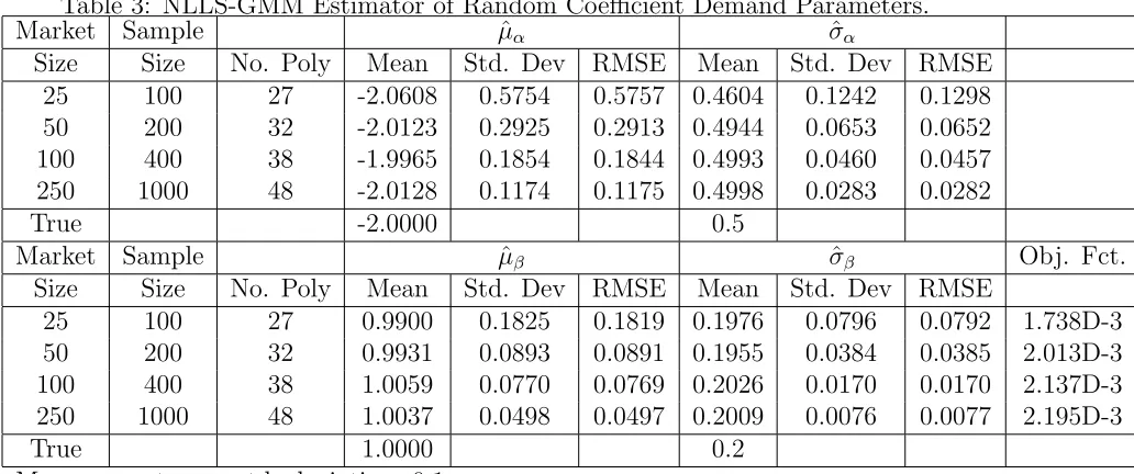
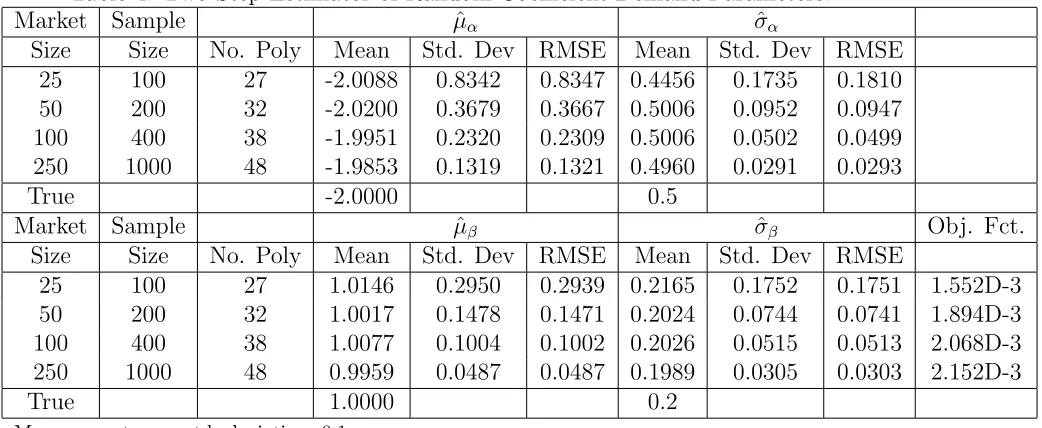
Through a set of Monte-Carlo experiments, we illustrate how our estimator delivers

consistent parameter estimates when demand shock is not only correlated with equilibrium

price and output, but also with cost shock, input prices and market size, and when cost

shock is correlated with market size. In such a setting there are no valid instruments to

account for price endogeneity, and market size alone cannot control for the supply side.

The IV estimates, on the other hand, are shown to have bias.8

A prominent example of papers that exploit first order conditions to estimate demand

parameters is Smith (2004). He estimates a demand model using consumer-level choice

data for supermarket products. He does not, however, have product-level price data.

To overcome this missing data problem, he develops a clever identification strategy that

uses data on national price-cost margins, and identifies the price coefficient in the demand

model as the one that rationalizes these national margins.9 Our study differs considerably

in that we focus on the more common situation where a researcher has data on prices,

aggregate market shares and total costs, but not marginal costs. Indeed, we directly build

on the general BLP framework.

This paper is organized as follows. In Section 2, we specify the differentiated products

model of interest and review the IV based estimation approach in the literature. In Section

3, we study identification when demand and cost data are available and develop our formal

identification results. Section 4 proposes estimators that are based on our identification

arguments and analyzes the large sample properties of our preferred NLLS-sieve estimator.

Section 5 contains a Monte-Carlo study that illustrates the effectiveness of our estimator

in environments where standard approaches to demand estimation yield biased results.

In Section 6 we conclude and discuss potential applications of our estimator.

8_{A further result from our experiments speaks to the relative numerical performance of ours and}

IV estimators. Whereas we easily obtain convergence in our estimation routines, for most Monte-Carlo samples, like Dube et al. (2012) and Knittel and Metaxoglou (2012) we find the BLP algorithm to be quite unstable.

9_{Genesove and Mullin (1998) use data on marginal cost to estimate the conduct parameters of the}

2

Differentiated products models and IV estimation

2.1

Differentiated products models

Consider the following standard differentiated products discrete choice demand model.

Consumer i in market m gets the following utility from consuming one unit of product j

uijm =x0jmβ+αpjm+ξjm+ijm, (1)

where xjm is a K ×1 vector of observed product characteristics, pjm is price, ξjm is the unobserved product quality (or demand shock) that is known to both consumers and firms

but unknown to researchers, and ijm is an idiosyncratic taste shock. Denote the demand parameter vector by θ = [β0, α]0 whereβ is a K×1 vector.

Suppose there are m = 1. . . M isolated markets that have respective market sizes

Qm.10 Each market hasj = 0. . . Jm products whose aggregate demand across individuals is

qjm =sjmQm,

where qjm denotes output and sjm denotes market share. In the case of the Berry (1994) logit demand model which assumes ijm has a logit distribution, the aggregate market share for product j in market m is

sjm(θ)≡s(pm,Xm,ξm, j,θ) =

exp x0_jmβ+αpjm+ξjm

PJm

k=0exp (x

0

kmβ+αpkm+ξkm)

= exp (δjm)

PJm

k=0exp (δkm)

, (2)

where pm = [p0m, p1m, ..., pJmm]

0 _{is a (J}

m+ 1)×1 vector, Xm = [x0m,x1m, ...,xJmm]

0 _{is a}

(Jm+ 1)×K matrix, ξm= [ξ0m, ξ1m, ..., ξJmm]

0 _{is a (J}

m+ 1)×1 vector, andδjm =x0jmβ+

αpjm+ξjm is the “mean utility” of productj. Notice from the definition of mean utility that we can also denote the market share equation by s(δm(θ), j)≡s(pm,Xm,ξm, j,θ) where δm(θ) = [δ0m(θ), δ1m(θ), . . . , δJmm(θ)]

0 _{is a J}

m+ 1×1 vector of mean utilities.

Following standard practice, we label good j = 0 as the “outside good” that corre-sponds to not buying any one of the j = 1, . . . , Jm goods. We normalize the outside good’s product characteristics, price, and demand shock to zero (i.e., x0m =0, p0m = 0,

and ξ0m = 0 for all m), which implies δ0m(θ) = 0. This normalization, together with the logit assumption for the distribution of ijm, identifies the level and scale of utility.

In the case of BLP, one allows the price coefficient and coefficients on the observed

characteristics to be different for different consumers. Specifically, α has a distribution function Fα(.;θα), where θα is the parameter vector of the distribution, and similarly,

β has a distribution function Fβ(.;θβ) with parameter vector θβ. The probability a consumer with coefficients α and β purchases product j is identical to that provided by the market share formula in equation (2). The aggregate market share is obtained by

integrating over the distribution of α and β,

s(pm,Xm,ξm, j,θ) = ˆ

α ˆ

β

exp x0_jmβ+αpjm+ξjm

PJm

j=0exp x

0

jmβ+αpjm+ξjm

dFβ(β;θβ)dFα(α;θα). (3)

Often the distributions of α and each element of β are assumed to be independently normal, implying that the parameters consist of mean and standard deviation, i.e., θα =

[µα, σα]0, θβk = [µβk, σβk]0, k = 1, ..., K. The mean utility is then defined to be δjm =

x0_jmµ_β +µαpjm+ξjm, with δ0m = 0 for the outside good.

2.1.1 Recovering demand shocks

Given θ and data on market shares, prices and product characteristics, we can solve for

the vectorδmthrough market share inversion. This involves findingδm for marketmthat solves s(δm,θ)−sm = 0, where sm = (s0m, s1m, ..., sJmm)

0

is the observed market share

and s(δm(θ), j,θ) is the market share of firm j predicted by the model. That is, market share inversion involves solving the following set of Jm equations,

s(δm(θ), j,θ)−sjm = 0, for j = 0, . . . , Jm, (4)

and therefore,

δm(θ) =s−1(sm,θ), (5)

The vector of mean utilities that solves these equations perfectly aligns the model’s

pre-dicted market shares to those observed in the data.

utilities for productj using its market share and the share of the outside good asδjm(θ) = log(sjm)−log(s0m), j = 1, . . . , Jm (with δ0m normalized to 0). In the random coefficient case, there is no such closed form formula for market share inversion. Instead, BLP

propose a contraction mapping algorithm that recovers the unique δm(θ) that solves (5)

under some regularity conditions.

With mean utilities in hand, recovering the structural demand shocks is

straightfor-ward,

ξjm(θ)≡ξ(pm,Xm,ξm, j,θ) = δjm(θ)−x0jmβ−αpjm (6) for the logit model. For the BLP model, we use µ_β instead of β and µα instead of α as coefficients. That is,

ξjm(θ)≡ξ(pm,Xm,ξm, j,θ) =δjm(θ)−xjm0 µβ −µαpjm (7)

2.1.2 IV estimation of demand

A simple regression of δjm(θ) = x0jmβ+αpjm +ξjm with δjm(θ) being the dependent variable and x0_jm and pjm being the regressors would yield a biased estimate of the price coefficient. This is because firms likely set higher prices for products with higher

unob-served product quality, which creates correlation betweenpjm and ξjm.

Researchers use a variety of demand instruments to overcome this issue. That is, using

the inferred values ofξjmfor all products and markets, we can construct a GMM estimator for θ by assuming the following population moment conditions are satisfied at the true

value of the demand parameters θ0: E[ξjm(θ0)zjm] = 0, where zjm is an L×1 vector of instruments. However, good instruments are not easy to find, as we discuss below.

Cost shifters are often used as instruments. This is in line with traditional market

equilibrium analysis which identifies the demand curve from shifts in the supply curve.

Popular examples are input prices, wjm. However, one cannot rule out the possibility

that the exclusion restriction of cost shifters in the demand function does not hold. Input

prices, like wages, may affect demand of products in the same local market through

changes in consumer income. Changes in other input prices such as gasoline or electricity

firms to reduce unobserved product quality, and hence could also undermine the exclusion

restriction.

In instances where cost shifters are likely to satisfy the exclusion restriction, they are

often weak instruments. For example, if one assumes that input prices are exogenously

determined in external labor and capital markets, then all firms will face the same input

prices. Therefore, cost shifters may not have sufficient within-market variation across

firms to identify the demand parameters, especially if market fixed effects are included in

the utility function in (1).

BLP originally proposed using product characteristics of rivals’ products as price

in-struments. As we can see in equation (3), a firm’s market share is a function of prices

and observed product characteristics of all firms in its market. Therefore, the exclusion

restriction that enables one to use rivals’ product characteristics as price instruments

heav-ily depends on functional form assumptions for the utility function and the distribution

function of utility shocks.

A further potential issue with these instruments is that product characteristics, like

prices, may be chosen strategically by firms. Indeed recently a literature on endogenous

characteristics has emerged,11 which raises concerns that product characteristics are also

endogenous. In this case, IVs are needed for prices as well as product characteristics for

identification.

A final commonly-used set of instruments is the set of prices of product j in markets other than m (Nevo (2001); Hausman (1997)). The strength of these instruments comes from common cost shocks for products across markets that create cross-market correlation

in product prices. However, researchers need to ensure they use such instruments in cases

where there is no spatial correlation in demand shocks across markets as this would render

these instruments invalid. Regional demand shocks or national marketing campaigns, for

example, could generate such correlation.12

11_{See Crawford (2012) for an overview of this literature.}

12_{Firm, market, and year fixed effects are typically included in the set of instruments when panel}

2.2

Supply

The cost of producingqjm units of productj in marketm,Cjm, is assumed to be a strictly increasing function of output, L×1 vector of input prices wjm, and a cost shock υjm. That is,

Cjm =C(qjm,wjm, υjm,τ), (8) where τ is the cost parameter vector. In addition, C() is assumed to be continuously differentiable with respect to output.

Given this cost function and the demand model above, we can write firm j’s profit function as

πjm =pjm×s(pm,Xm,ξm, j,θ)×Qm−C(s(pm,Xm,ξm, j,θ)×Qm,wjm, υjm,τ), (9)

where we assume there is one firm for each product. Keeping with BLP, we for now

assume that firms act as differentiated products Bertrand price competitors. Therefore,

the optimal price and quantity of productj in marketmare determined by the first order condition (F.O.C.) that equates marginal revenue and marginal cost

pjm+sjm

∂s(pm,Xm,ξm, j,θ)

∂pjm

−1

| {z }

M Rjm

= ∂C(qjm,wjm, υjm,τ)

∂qjm

| {z }

M Cjm

. (10)

Note thatM Rjm in (10) can be written solely as a function of prices, market shares and parameters. This is because, given the market share inversion in (5), and the specification

of mean utility δjm, demand shock ξm is a function of Xm, pm, sm and θ. Therefore, marginal revenue can be written as

M Rjm ≡M Rjm(θ)≡M R(pm,sm,Xm, j,θ). (11)

This turns out to be quite useful in developing our identification and estimation approach

below. Also, equations (10) and (11) imply that demand parameters can potentially be

identified if there is data on marginal cost or even without such data, if the cost function

2.2.1 Cost function estimation

As with demand estimation, a similar inversion procedure can be used to recover

unob-served cost shocks,

Cjm=C(qjm,wjm, υjm,τ)⇒υjm(τ) =C−1(qjm,wjm, Cjm,τ). (12) Like demand estimation, there are important endogeneity concerns with standard

ap-proaches to estimating cost functions. Specifically, outputqjmis endogenously determined by profit maximizing firms equating marginal revenue to marginal cost as in equation (10),

and is potentially negatively correlated with the cost shockυjm. That is, all else equal, less efficient firms tend to produce less. In dealing with this issue, researchers have

tradition-ally focused on selected industries where endogeneity can be ignored, or used instruments

for output.

The IV approach to cost function estimation typically uses excluded demand shifters

as instruments. We denote this vector of cost instruments by ˜zjm. We can estimate τ

assuming that the following population moments are satisfied at the true value of the

cost parameters τ0: E[υjm(τ0)˜zjm] = 0. This approach potentially has pitfalls that are similar to the ones we discussed with IV demand estimation. In particular, typical

excluded demand shifters such as demographics affect all firms, and thus generate little

within-market, across-firm variation in equilibrium output for identification. Moreover,

one cannot completely rule out the possibility of correlation between demand shifters and

cost shocks.

3

Identification and estimation of the price

coeffi-cient

In this section, we investigate the benefits of jointly using demand and cost data to

identify the model. It turns out that the endogeneity concerns in estimating the demand

and cost parameters can be mitigated if the parameters are jointly estimated using such

data. Fundamental to this result is having variation in market size across markets, which

The identification analysis is developed in three parts. For now we focus solely on

identification of the price coefficient; later we extend the analysis to include other

de-mand parameters such as the coefficients on product characteristics, and cost function.

First we present the main idea for our general identification results in a simple monopoly

model with Berry (1994) logit demand. We then maintain the simple logit demand

struc-ture, and prove identification under various extensions to the supply-side of the model:

oligopoly, cost data with measurement error and systematic misreporting, and fixed costs.

Second, we prove identification in a setting with a richer BLP/random coefficients model

of demand. Here we emphasize the need to assume that marginal revenue identifies the

price coefficient and show this assumption holds for logit and BLP demand. Third, we

show the marginal revenue and market share functions are in fact non-parametrically

iden-tified. We find, however, that the estimation strategy that directly follows our parametric

or nonparametric identification argument is likely to be subject to a Curse of

Dimension-ality in practice. This motivates us to pursue a different parametric estimation strategy

in Section 4.

3.1

Identification in the Logit model

3.1.1 Main assumptions

We begin by considering identification in the simplest possible environment: a monopolist

who sells one product and faces logit demand. The following six assumptions are the main

ones needed for identification in this model and its extensions.

Assumption 1 Researchers have data on outputs, product prices, market shares, input

prices, and observed product characteristics of firms. In addition, data on firms’ total cost

are available.

Assumption 2 Marginal revenue is a function of observed product characteristics,

prod-uct prices and market shares. Marginal cost is a function of output, input prices and cost

shock.

Assumption 3 The cost function is strictly increasing, continuously differentiable in

Assumption 4 Markets are isolated. Market size is not a deterministic function of

de-mand/supply shocks, and/or dede-mand/supply shifters.

We denote M Cjm to be the marginal cost of firm j in market m, i.e. M Cjm =

M C(qjm,wjm, υjm).

Assumption 5 Firms set prices such that marginal revenue is a function of marginal

cost, taking as given their rivals’ prices. That is, M Rjm =ζ(M Cjm).

Assumption 6 The support of the supply shock υjm is in R+ and the support of the demand shock ξ_m is in RJm_{. However, only firms that have p}

m, sm, Xm, υjm and ξm such that under the true parameter vector θ0, δ0−1 ≤

h

∂lns(pm,Xm,ξm,j,θ0)

∂lnpjm

i−1

≤ −δ0 for

a small δ0 > 0, are observed in the market. The rest of the firms are out of the market.

Furthermore, for the sake of simplicity, we assumeα0 <0for the logit model and µα0 <0

for the BLP random coefficient model.13

For simplicity, throughout, we also assume that firms in the same market m share the common input price vector wm. This assumption can be weakened without changing any

of the results below.

3.1.2 Monopoly

The intuition for how the price coefficient can be identified by using demand and cost data

jointly can be illustrated with a single-product monopolist facing logit demand. Assuming

for the moment that the monopolist maximizes profits, the following first order condition

holds in equilibrium:

M R(pm,sm,Xm,θ0) =pm+

1 (1−sm)α0

=M C(qm,wm, υm), qm =Qmsm,

13_{Assumption 6 is not often discussed in the BLP setup. If we generate demand shocks that have}

reasonably large variance and are independent of other exogenous variables and cost shocks, then even for many parameter values with negativeµα some outcomes will have market shares with positive slope

with respect to price. In effect, previous researchers may have either: (1) allowed positive slopes to occur in the data; (2) implicitly avoided parameters that generate these anomalies; or (3) implicitly assumed that only demand shocks that generate negative slope are selected in the data. The latter two strategies potentially result in bias of the price coefficient estimate. As we will see later, since our identification and estimation strategy of the price coefficient does not use any orthogonality conditions involving demand shocks, it is not subject to this form of selection bias. However, our estimator forβorµβwill be subject

where α0 is the true price coefficient. We use the exclusion restriction that the

monop-olist’s market share sm does not directly enter in the marginal cost function, and its outputqm does not directly enter in the marginal revenue equation. It is the market size

Qm that provides the link between market share and output, and variation between the two. Now, suppose there were no cost shocks. That is, the marginal cost function is

M C(qm,wm). Then, if we find a pair of monopolists in different markets with different market sizes, prices and market shares but with the same output and input price vector,

then we know they must have the same marginal cost. Thus, the equality of marginal

revenue to marginal cost implies

pm+

1 (1−sm)α0

=pm0+

1 (1−sm0)α₀

, α0 =−

1

pm−pm0

1 1−sm

− 1

1−sm0

(13)

and the price coefficient α0 is identified.

The same argument cannot be made in the presence of a cost shock υm to M Cm, i.e.

M Cm = M C(qm,wm, υm). Then, marginal costs of two firms with the same output qm and input prices wm will not be equal, thus, for these two firms, equation (13) will not

hold. In order to allow for a cost shock, we modify this identification argument and pair

up firms that have differentQmandsm, but have the sameqm,wm and Cm. It follows that these firms must have the same cost shock, and thus, we can identify the price coefficient

with equation (13)

Note that we have assumed profit maximization for expositional purposes only. It is not

required for identification. Assumption 5 ensures that if we pair firms such that they have

the same output, input prices, total cost and (hence) cost shock, then M Cm =M Cm0⇒

M Rm =M Rm0 and we can identify the price coefficient using equation (13).

3.1.3 Oligopoly

We now extend the identification argument to the oligopoly case, where in market m

there are Jm firms selling one product each.14. Let Cjmd be the observed cost, and let

Pjm ={Qm, qjm,wm,pm,sm,Xm, j}contain the other relevant information (beyond cost) about firm j in market m.

In addition to Assumptions 1-6, identification in the oligopoly case relies on the

fol-lowing assumption,

Assumption 7 There exists a pair of observations Pjm = {Qm, qjm,wm,pm,sm,Xm, j} and Pj0_m0 ={Q_m0, q_j0_m0,w_m0,p_m0,s_m0,X_m0, j0} that satisfy w_m =w_m0, q_jm =q_j0_m0, Cd

jm =

C_jd0_m0 and p_jm6=p_j0_m0.

Going forward, we drop the cost parameter vectorτ as we will treat the cost function

C(·) as nonparametric for the remainder of the paper.

Proposition 1 Suppose Assumptions 1-7 are satisfied. Then, wm = wm0, q_jm = q_jm0,

C_jmd = C_jd0_m0 implies υjm = υj0_m0, where υ_jm is the cost shock corresponding to the set of observations Pjm, and υj0_m0 for P_j0_m0. Further, under the logit demand model the true price coefficient α0 is identified by

α0 =−

1

pjm−pj0_m0

1 1−sjm

− 1

1−sj0_m0

. (14)

Proof. Suppose υjm> υj0_m0. Then, since the cost function is strictly increasing in υ,

C(qjm,wm, υjm) =C(qj0_m0,w_m0, υ_jm)> C(q_j0_m0,w_m0, υ_j0_m0),

contradicting Cd

jm = Cjd0_m0. A similar contradiction obtains for υ_jm < υ_j0_m0. Therefore,

υjm =υj0_m0. Thus,

M C(qjm,wm, υjm) =M C(qj0_m0,w_m0, υ_j0_m0).

Because M R = ζ(M C) by Assumption 5, if data points jm and j0m0 have the same marginal cost then they must have the same marginal revenue. In the case of logit model,

this implies

pjm+

1 (1−sjm)α0

=pj0_m0 +

1 (1−sj0_m0)α₀

.

It then follows that α0 is identified from such a pair of data points as follows

α0 =−

1

pjm−pj0_m0

1 1−sjm

− 1

1−sj0_m0

The above result highlights the importance of the variation of market size for

iden-tification. If all the data came from a single market, or from two markets of the same

size, then qjm =qj0_m0 implies s_jm =s_j0_m0, thus p_jm = p_j0_m0 if α₀ 6= 0 and thus α₀ cannot

be identified from (14), unless the true value is α0 = 0. The example also illustrates the

role of cost data in identifying the price coefficient. As long as we can find firms with the

same cost, output, and input price, they will have the same cost shock and marginal cost,

thereby allowing us to difference away their supply side effects in a pairwise fashion.

What Assumption 7 states is that there exist two markets m,m0 with different market sizesQm 6=Qm0 with two firmsjm, j0m0 that have the same input price vectorw_m =w_m0

and the same output qjm = qj0_m0, but potentially different vectors of demand shocks

ξ_m 6= ξ_m0, thus, different market shares s_m 6=s_m0. Two such firms can exist even if we

allow for correlation between the input price and the cost shocks. In the same manner,

correlation between demand shocks and input price, or between demand shocks and cost

shocks do not prevent us from finding pairs of firms satisfying Assumption 7, as long as

there is sufficient variation in market size and demand shocks.

In addition to allowing for such correlation between observables and unobservables

within markets, our approach also allows demand and cost shocks to be correlated across

markets, as long as the correlation is not perfect. Further yet, we do not need to assume

exogeneity of Xm to identify α as is typically assumed. In sum, these findings illustrate that given cost data, one does not need any conventional IV- or orthogonality assumptions.

And, as long as marginal revenue is a function of, but not necessarily equal to, marginal

cost, we can identifyα without assuming profit maximization. This makes our framework applicable to firms that are under government regulation and firms under organizational

incentives or behavioral aspects that prevent them from maximizing profit.

We note that, in practice, Assumption 7 is unrealistic. However, a similar argument

can be made for pairs that satisfy the equalities in Assumption 7 approximately.

3.1.4 Measurement error and misreporting in costs

Two important issues are likely to arise in practice with the above identification strategy.

different estimate of α. This would immediately lead a practitioner to conclude that the model is misspecified since, if the model is correct, it is impossible to have two such pairs

of markets that deliver differentαestimates. This issue arises because the specification of the model is too strong. According to the model, given output and input price, cost data

uniquely identify cost shocks. Second, it is widely accepted that cost data are measured

with error.

In light of these issues, we weaken the model specification by allowing for both

mea-surement error as well as systematic misreporting of true costs. The following assumption

generalizes our cost function specification.

Assumption 8 The observed cost of firm j in market m, Cd

jm differs from the true cost

Cjm as follows.

C_jmd =ϕ(Cjm) +ηjm. (15) where ϕ is a strictly increasing function and measurement error ηjm is i.i.d. distributed with mean 0 and variance σ2

η. In addition, we assume measurement error is independent

of {qjm,wjm,pm,sm,Xm, j}, for all j, m.

So, for example, if firms report costs truthfully but with error then ϕ(C) = C. Alter-natively, if firms systematically under-report their true costs, then we could consider a

specification likeϕ(C) =ϕC where 0< ϕ <1. Over-reporting could be captured by the same specification, but where ϕ >1.

It turns out that in order to identify the price coefficient given cost data characterized

by Assumption 8, the only modification we need to make to our identification argument is

that we work with firms with the same mean cost conditional on{qjm,wjm,pm,sm,Xm, j}, rather than firms with the same cost data. Assumption 9 formalizes this requirement.

Assumption 9 There exist two firms with P ={Qm, qjm,wm,pm,sm,Xm, j}

and P0 = {Qm0, q_j0_m0,w_m0,p_m0,s_m0,X_m0, j0}, where q_jm = q_j0_m0, w_m = w_m0, p_m 6= p_m0 and

ECd|qjm,wm,pm,sm,Xm, j

=ECd|qj0_m0,w_m0,p_m0,s_m0,X_m0, j0.

Proof. The proof is very similar to that of Proposition 1. Since the measurement errors

are i.i.d. and independent of {qjm,wm,pm,sm,Xm, j} and {qj0_m0,w_m0,p_m0,s_m0,X_j0, j0},

ECd|qjm,wm,pm,sm,Xm, j

=E[(ϕ(C(qjm,wm, υjm)) +η)|qjm,wm,pm,sm,Xm, j] =ϕ(C(qjm,wm, υjm)).

Similarly,

E

Cd|qj0_m0,w_m0,p_m0,s_m0,X_j0, j0=ϕ(C(q_jm,w_m, υ_j0_m0)).

By Assumption 9,

ECd|qjm,wm,pm,sm,Xm, j

=ECd|qj0_m0,w_m0,p_m0,s_m0,X_j0, j0.

Thus, given qjm =qj0_m0, w_m =w_m0, and ϕ() being an increasing function, it follows that

υjm =υj0_m0. Therefore,

M C(qjm,wm, υjm) =M C(qj0_m0,w_m0, υ_j0_m0),

and,

α0 =−

1

pjm−pj0_m0

1 1−sjm

− 1

1−sj0_m0

,

and the price coefficient α0 is identified.

The conditional mean function ECd_{|q,w,p,s,X, j}

can be recovered from the data

by kernel or sieve based regression where the dependent variable is the cost data Cd and the independent variables are sieve polynomials of (q,w,p,s,X). In practice, this would likely be subject to a Curse of Dimensionality.

3.1.5 Fixed costs

We can further extend the above identification argument to include a fixed cost. To begin,

we denote fixed costs as

where ς_jmF is independent of υjm, and wlog, has mean zero. The modified cost function that includes variable and fixed costs is

˜

C(qjm,wm, υjm) +ςjmF ≡C(qjm,wm, υjm) +F (υjm) +ςjmF .

where ˜C(qjm,wm, υjm) ≡ C(qjm,wm, υjm) +F(υjm) and the relationship between the observed and true costs is updated to be

C_jmd =ϕC˜(qjm,wm, υjm) +ςjmF

+ηjm.

That is, we allow for the systematic misreporting of the true cost, which now includes the

random term of the fixed cost, ςF jm.

In this set-up, as long as ˜Cjm ≡C˜(qjm,wm, υjm) satisfies Assumption 3 then Propo-sition 2 holds. To see why, first note that

E_(ςF_,η) h

ϕC˜jm+ςF

+η|C˜jm

i

> E_(ςF_,η) h

ϕC˜j0_m0 +ςF

+η|C˜j0_m0

i

implies

E_ςF h

ϕC˜jm+ςF

i

> E_ςF h

ϕC˜j0_m0 +ςF

i

.

Becauseϕ() is an increasing function, this implies ˜Cjm >C˜j0_m0. The opposite inequalities

also hold. That is,

E_(ςF_,η) h

ϕC˜jm+ςF

+η|C˜jm

i

< E_(ςF_,η) h

ϕC˜j0_m0 +ςF

+η|C˜j0_m0

i

implies ˜Cjm <C˜j0_m0. Therefore,

E(ςF_,η) h

ϕC˜jm+ςF

+η|C˜jm

i

=E(ςF_,η) h

ϕC˜j0_m0 +ςF

+η|C˜j0_m0

i

implies ˜Cjm = ˜Cj0_m0. Therefore,

˜

and the same identification proof from Proposition 2 goes through.

3.2

Identification of marginal revenue

We now enrich the demand-side of the model, and show that parameters of the distribution

of price coefficients in the BLP model are identified as well. As with the logit model, the

identification analysis has two parts. The first part, which is related to supply, concerns

finding pairs of firms with the same output, input price vector and conditional mean

cost. The second part, which is related to demand, concerns whether price coefficients

can be identified from these firm pairs with the same marginal revenue. Since the cost

function is nonparametric, the first part of the analysis remains unchanged for different

parametric demand specifications. Only the second part changes, for which we present

general conditions for identification. We then show that the logit and BLP demand model

satisfy these conditions.

3.2.1 General conditions for identification

We make the following assumptions on the support of the market size, demand and

cost shock, and marginal cost. These greatly simplify the identification proofs without

imposing any orthogonality restrictions.

Assumption 10 The following properties hold for all jm:j = 1, . . . , Jm, m= 1, . . . , M. Let X = (X1, . . . ,Xm). Let the vector of market size of all markets other than m be

Q−m = (Q1, Q2, . . . , Qm−1, Qm+1, . . . QM). Similarly let the vector of input prices of all markets other than m be denoted as W−m = (w1,w2, . . . ,wm−1,wm+1, . . .wM). Let the vector of demand shock of all firms other thanjmbeΞ−j,−m = ξ01, . . . ,ξ

0

m−1,ξ

0 −jm,ξ

0

m+1, . . .ξ

0

M

,

where ξ_−jm is the vector of demand shocks of all firms in market m other than the firm

Furthermore, the support of the input price wm given Qm, ξjm, υm and V−j,−m is RL+,

where L is the number of inputs.

Assumption 11 For anyq >0, w>0, the marginal cost function satisfies the following properties:

limυ↓0M C(q,w, υ) = 0, limυ↑∞M C(q,w, υ) =∞.

Furthermore,

limM C↓0ζ(M C) = 0, limM C↑∞ζ(M C) =∞.

The key identification assumption for a general parametric demand function is that

marginal revenue identifies the price coefficient. That is, one can find two vectors of

prices, market shares and matrices of observed characteristics that have the same marginal

revenue under the true price parameters, but different marginal revenues under the wrong

price parameters. We introduce some notation before stating this assumption formally.

Let the parameter vector have two components, θ = (θ−p,θp)∈Θ−p×Θp where Θ−p is the parameter space ofθ−p andΘp is the parameter space ofθp. Roughly,θp corresponds

to the price coefficient that we identify below.

Let ν and ν0 be two sets of vectors of prices, market shares, and observed product

characteristics that can be generated as an equilibrium of the oligopoly model under

corre-sponding assumptions, withJrows for the former andJ0 rows for the latter, corresponding to two markets,

ν ={p,s,X}, ν0 ={p0,s0,X0}, ν 6=ν0.

Assumption 12 For any given θp 6=θp0, there exist ν and ν0,ν 6=ν0, andj that satisfy

the following properties.

1. pl > 0, 0 < sl < 1 for l = 1, ..., J and p0l > 0, 0 < s

0

l < 1, for l = 1, .., J

0_{, and}

0<PJ

l=1sl <1, 0<

PJ0

l=1s

0

l<1.

2. For any θ−p ∈Θ−p,

M R(p,s,X, j,θ−p,θp0) = M R(p0,s0,X0, j,θ−p,θp0)

where θ0 = (θ−p0, θp0) is the true parameter vector.

Proposition 3 Suppose cost data is generated as in equation (15), and Assumptions 1-6

and Assumption 10-12 are satisfied. Then, θp0 is identified.

Proof. See Appendix

3.2.2 Identification in the logit and BLP model

It is important to note that Assumption 12 is a high level assumption; it is not necessarily

satisfied in all demand models. For example, if marginal revenue is a multiplicative,

separable function of θp, then θp is not identifiable by MR. To see this, notice that for

any θp, and for any (p,s,X) and (p0,s0,X0), M R(p,s,X, j,θ) = M R(p0,s0,X0, j,θ) implies M R(p,s,X, j,θ−p)g(θp) = M R(p0,s0,X0, j,θ−p)g(θp) for some g(·). Hence, Assumption 12 is violated.

The marginal revenue function for logit and BLP does not have a multiplicative,

separable form, nor do most functions commonly used by researchers. The important

question, then, is whether the logit and BLP demand models satisfy Assumption 12. The

proposition below answers this question for the monopoly case.

Proposition 4 Suppose Assumptions 1-6 and Assumptions 10-11 are satisfied, and there

exist two firms jm and jm0 with demand variables νm = {pm,sm,Xm} and νm0 =

{pm0,s_m0,X_m0} where p_jm 6=p_jm0. Then,

a. Assumption 12 is satisfied for the logit model for monopoly markets.

b. Assumption 12 is satisfied for the BLP model without observed product characteristics

for monopoly markets if sm 6=sm0 and

η0 ≡

µα0

σα0

<− 1

2φ(0). (16)

Proof. See Appendix.

We can further include controls Xm into the demand model, and show that the cost

data identifies parameters of the random coefficients on price (µα, σα), as well as σβ, the

we formally prove identification when the observed product characteristicxjm is a scalar for all firms jm. As we can see from equations (6) and (7), what is not identified from the cost data alone is µ_β. This is because given (µα, σα), and σβ, only ξjm+x0jmµβ is identified without further restrictions imposed from the model.

Proving Assumption 12 for the BLP model with oligopoly markets is a straightforward

extension of Proposition 4 and is thus omitted. It requires data that contain firms with

high and similar prices: p1m = p2m = ...pJmm = p for sufficiently high p. Despite the

need for these strong assumptions in the formal argument for parametric identification of

the BLP model, we later show that the parameters are well-identified in our Monte-Carlo

experiments.15

Next we prove nonparametric identification to illustrate that identification of the

de-mand function does not rely on its functional form restrictions like logit or BLP. Readers

who are more interested in our new estimation procedure can skip Subsection 3.3 and

directly move to Section 4.

3.3

Nonparametric identification of marginal revenue function

In this section, we show that marginal revenue is nonparametrically identified, and that the

market share function can be recovered from nonparametric marginal revenue estimates.

To simplify our discussion, we again first focus on monopoly markets and then extend our

identification arguments to oligopoly markets.

We begin by making the following auxiliary assumptions for the monopoly model:

Assumption 13 LetM R(p,x, ξ)be the marginal revenue specified as a function of price

p, vector of product characteristics x and the demand shock ξ.

a. M R(p,x, ξ) is strictly increasing in p.

b. For any x, x0 and two pairs of prices and market shares (p, s) and (p0, s0) such that

15_{The proof for the BLP model relies on firms with very high prices for identification. This is}

s=s0 and p > p0,

M R(p,x, ξ(p, s,x))> M R(p0,x0, ξ(p0, s0,x0)).

where recall the demand shock ξ is an unspecified function of p, s and x.

Assumption 14 The market share function s(p,x, ξ) is strictly decreasing and continu-ous in p and strictly increasing and continuous in ξ. Furthermore,

limξ↓−∞s(p,x, ξ) = 0, limξ↑∞s(p,x, ξ) = 1 and limp↑∞s(p,x, ξ) = 0.

Assumption 15 Firms maximize profits, setting prices to equate marginal revenue and

marginal cost. Furthermore,

C_jmd =C(qjm,wjm, υjm) +ηjm

where E(ηjm|qjm,wjm, υjm) = 0

Assumption 30 For any w, the marginal cost function is nondecreasing and continuous

in q and increasing and continuous in υ. Furthermore, for any w>0, and q >0,

limυ↓0M C(q,w, υ) = 0, and limυ↑∞M C(q,w, υ) =∞.

Given these additional assumptions, we prove that marginal cost and marginal revenue

are nonparametrically identified. The following proposition formally states our claim.

Proposition 5 Suppose Assumptions 1, 2, 30, 4, 5, 6 and Assumptions 13, 14 and

15 are satisfied. Consider a monopolist in market m with the set of observables Pm = {Qm,wm, qm, pm, sm,x}, and demand shock and cost shock ξm and υm, respectively.

a. Suppose the marginal cost is increasing in output. Then consider the monopolist firm

ξm =ξ) and cost shock (υm0 =υ_m =υ) but has a different market size Q_m0 > Q_m. It follows that

sm > sm0, p_m < p_m0, q_m < q_m0, (17) and

pm

1 + lnpm0−lnpm

lnsm0−lns_m

=E

Cd_|q

m0,w_m0, p_m0, s_m0,x_m0−ECd|q_m,w_m, p_m, s_m,x_m

qj0_m0−q_m

+O(|Qm0 −Q_m|). (18)

b. Suppose the marginal cost is increasing in output. Suppose we have a firm m0 with

Pm0 close to P_m, such that both (17) and (18) hold. Then, the true marginal cost at

{Qm,wm, qm, pm, sm,xm}, M Cm satisfies

M Cm =

E

Cd_|q

m0,w_m0, p_m0, s_m0,x_m0−ECd|q_m,w_m, p_m, s_m,x_m

qm0−q_m

+O(|Qm0 −Q_m|),

and the nonparametric estimate of M Cm is given by,

d

M Cm =

ECd_|q

m0,w_m0, p_m0, s_m0,x_m0−ECd|q_m,w_m, p_m, s_m,x_m

qm0 −q_m

(19)

c. Suppose the marginal cost is constant in output. Then consider another firm m0 with

Pm0 = {Q_m0,w_m0, q_m0, p_m0, s_m0,x_m0} close to P_m, that is generated by the same de-mand shock (ξm0 =ξ_m =ξ) and cost shock (υ_m0 =υ_m =υ) and that has a different market size Qm0 6=Q_m. It follows that

sm0 =s_m, p_m0 =p_m, q_m0 =Q_m0s_m0, (20)

and

M Cm =

ECd|qm0,w_m0, p_m0, s_m0,x_m0−ECd|q_m,w_m, p_m, s_m,x_m

qm0 −q_m

. (21)

Proof. See Appendix.

identified.16 That is, parts a and b say that for a point Pm in the population, if we can find a nearby pointPm0 with the samexand w, satisfying some inequalities relating their

market shares, prices and outputs, and if the first order condition using these points is

approximately satisfied, then a nonparametric estimate of marginal cost can be computed

from these points as the local slope of the average cost, where the average is taken over

the total cost conditional on output, input price, observed product characteristics, prices,

and market shares in (19).

Part c of Proposition 5 states the following: if one cannot find Pm0 close toP_m where

the sample analog of marginal revenue equals marginal cost, and one finds a nearby point

whose prices and market shares are the same as Pm, but output is different, then it is likely that the marginal cost is a constant. Thus one can derive the marginal cost as in

equation (21).

In implementing the above identification approach, in practiceECd|qm,wm, pm, sm,xm

could be nonparametrically estimated in a first step. Given the profit maximization

as-sumption, we could then obtain a nonparametric marginal revenue estimate M Rd_m from

the corresponding marginal cost estimate in a second step, M Rdm =M Cdm.17

It is fairly straightforward to see that the logit model with a negative price coefficient

satisfies Assumptions 13 a and b. We conducted an extensive numerical analysis with the

BLP demand model with negative µβ in monopoly markets and found that in all cases we tried, Assumptions 13 a. and b. are satisfied as long as marginal revenue is positive.

However, we have not provided a formal proof, and thus one cannot completely rule out

the possibility of Assumption 13 being violated.

Fortunately, Assumption 13 b. can be tested. Consider two monopoly firms who have

the same input prices and product characteristics, and whose output, market size, and

market shares are close to each other. In particular, for the point{Qm, qm,wm, pm, sm,xm}, take another close point{Qm0, q_m0,w_m0, p_m0, s_m0,x_m0}that satisfiesQ_m =Q_m0,s_m =s_m0 =

s, thusqm =qm0, butp_m< p_m0. Then, ifE Cd|q_m,w_m, p_m, s_m,x_m< E Cd|q_m0,w_m0, p_m0, s_m0,x_m0,

16_{Notice that a marginal revenue function that is multiplicatively separable in price parameters and}

other parameters and variables, is now identifiable given the additional identification assumptions.

17_{Recall that with parametric identification, we only needed to assume that marginal revenue was a}

it implies that C(qm,wm, υm) < C(qm0,w_m0, υ_m0), thus, υ_m < υ_m0, and given q_m =

qm0, M R_m = M C(q_m,w_m, υ_m) < M C(q_m0,w_m0, υ_m0] = M R_m0, and Assumption 13 b

holds. If, on the other hand, EC_md|qm,wm, pm, sm,xm

≥EC_md0|q_m0,w_m0, p_m0, s_m0,x_m0,

then M Rm = M C(qm,wm, υm) ≥ M C(qm0,w_m0, υ_m0) = M R_m0 and Assumption 13

b does not hold. Therefore, by testing the hypothesis EC_md|qm,wm, pm, sm,xm

< ECd

m0|q_m0,w_m0, p_m0, s_m0,x_m0 given q_m =q_m0, one can test Assumption 13 b.

Furthermore, even if Assumption 13 does not hold, if it is reasonable to assume that

marginal cost does not vary with output locally around the point Pm, then one can still nonparametrically identify marginal cost, and thus marginal revenue by using equation

(21) in part c of Proposition 5.

3.3.1 Oligopoly

We next consider oligopoly models with Jm firms in market m. We apply the same argument wlog to firm j = 1 in two different markets m and m0 with variables P1m ≡

{Qm, q1m,wm, p1m, s1m,s−1m,p−1m,Xm}andP1m0 ≡ {Q_m0, q_1m0,w_m0, p_1m0, s_1m0,s_−1m0,p_−1m0,X_m0},

where s−1m and p−1m are vectors of market shares and prices of firms other than firm 1

in market m and likewise for s−1m0 and p_−1m0. As in Proposition 5, we need to find two

close points in the data that have the same product characteristics (Xm = Xm0 = X)

and input price vector (wm =wm0 = w). In addition, the two markets must satisfy the

following properties

Qm < Qm0, s_1m > s_1m0, p_1m < p_1m0, s_1mQ_m < s_1m0Q_m0 and p_−1m =p_−1m0,

as well as

p1m

1 +lnp1m0−lnp1m

lns1m0−lns_1m

= E

Cd_|q

1m0,w_m0,p_m0,s_m0,X_m0−ECd|q_1m,w_m,p_m,s_m,X_m

q1m0−q_1m +O(

|Qm0 −Q_m|).

Then, with only slight modifications to the proof of Proposition 5 for the monopoly case, we

can prove nonparametric identification of the marginal revenue function for the oligopoly case.

3.3.2 Recovering the market share function

We can use this marginal revenue estimate to recover a nonparametric estimate of the

market share function. Denote the nonparametric marginal revenue estimate of firm 1

evaluated at point (pm,sm,Xm) by M Rd(p_m,s_m,X_m,1). Using the definition of marginal

revenue, we can recover the derivative of the market share function at this point as

∂s(pm,Xm,ξm(pm,Xm, sm),1)

∂p1m

=

M R(pm,sm,Xm,1)−p1m

s1m

−1

.

A nonparametric estimate of the market share derivative around the pointpm,sm,Xm for firm 1 can then be calculated as

\

∂s(p,X,ξ(p, X, s),1)

∂p1

=X

m

" d

M R(pm,sm,Xm,1)−p1m

s1m

#−1

Kh(p−pm,s−sm,X−Xm)

P

nKh(p−pn,s−sn,X−Xn)

,

where Kh(·) is a kernel with bandwidth vector h.

We can use this nonparametric estimate of the market share derivative to recover a

nonparametric estimate of the demand function. Starting from the point ¯p,¯s,X¯ (where ¯

s=s p¯,X¯,ξ¯,1 for someξ¯), we derive the approximation of s p¯+ ∆p,X¯,ξ¯,1, that is, the market share of firm 1 with price vector ¯p+ ∆p where ∆p = [∆p1m,0, . . . ,0]0 and where ∆p1m is small. The approximation is computed as

ˆ

s1 ≡ˆs(¯p+ ∆p,X¯,ξ¯,1) = ¯s+

\

∂s(¯p,X¯,ξ¯,1)

∂p

0

∆p,

where ∂s\(¯p_∂,X¯_p,ξ¯,1) =

\ ∂s( ¯p,X,¯ξ,¯1)

∂p1 ,0, . . . ,0

0

. The market share function can be iteratively

recovered in a similar fashion, where at iterationk the share estimate at price ¯p+k∆p is

ˆ

sk ≡sˆ p¯+k∆p,X¯,ξ¯,1

= ˆs p¯+ (k−1) ∆p,X¯,ξ¯,1+

\

∂s p¯+ (k−1) ∆p,ξ¯,X¯,1

∂p

0

Then,

ˆ

s p¯+k∆p,X¯,ξ¯,1=s p¯+k∆p,X¯,ξ,¯,1 +

k

X

l=1 

 



\

∂s p¯+l∆p,sˆl−1,X¯,1

∂p −

∂s p+l∆p,X¯,ξ,1

∂p





0

∆p+O k∆pk2 

.

Therefore, with some additional assumptions on the regularity of the marginal revenue

function, one can show that

ˆ

s p¯+k∆p,X¯,ξ,1 =s p¯+k∆p,X¯,ξ,1+O kk∆pk2

+kop(1)k∆pk.

Hence, we can obtain a nonparametric market share function estimate given X and p.

3.3.3 Curse of Dimensionality

In practice, a nonparametric estimator for the demand and cost parameters based on

Proposi-tions 5 and 6 will likely suffer from a Curse of Dimensionality. To implement such an estimator,

one would need to obtain a nonparametric estimate of ECd|qjm,wm,pm,sm,Xm

. For most

markets of interest,Xm will contain a number of product characteristics across a non-negligible

number of firms. This makes the dimensionality problem potentially quite severe.

Because of this dimensionality issue, in estimation we pursue the common practice where

researchers use parametric restrictions to reduce the dimensionality of the estimation problem,

essentially transforming the nonparametric estimation exercise into a semi-parametric one. In

particular, we adopt the Berry (1994) logit or Berry et al. (1995) random coefficients demand

model. This relaxes the need to condition on the individual variablespm,sm,Xm in developing

our estimator; we only need to control for the marginal revenue M Rjm, which is a parametric

function of these variables.

4

Estimation

An estimation strategy that reflects the parametric identification results the closest is to

construct a pairwise differenced estimator that pairs up firms with similar outputs, input

market. That is,

θpJ M = argminθp∈Θp X

j,m

X

j0_,m0_:(j0_,m0_)6=(j,m)

M Rjm(θ−p,θp)−M Rj0_m0(θ_−p,θ_p)

2

Wh

qjm−qj0_m0,w_jm−w_j0_m0,E_bCd|q_jm,w_jm,p_m,s_m,X_m, j−

b

E

Cd|qj0_m0,w_j0_m0,p_m0,s_m0,X_m0, j0,X_jm−X_j0_m0

,

where Wh is the kernel based weight function with the vector of bandwidth beingh, and b

ECd_{|q,w,p,s,X, j}

is the sample average of cost data conditional on {q,w,p,s,X, j}. The advantage of the above estimator is that it recovers demand parameters even if the

firm is not profit maximizing, and thus, is potentially useful in industries where firms are

under government regulation.

However, the need for Eb

Cd_{|q,w,p,s,X, j}

makes the Curse of Dimensionality of

the estimator just as severe as the one for nonparametric identification discussed above.

Thus the estimator may be impractical in most oligopoly markets where number of firms

is sufficiently high. Therefore, from now on, we focus on developing an estimator that

works well in such situations. To do so, we need to find a way to condition on marginal

revenue, which is a parametric function of the observables, rather than the conditional

expected cost.

As a first step towards constructing such an estimator, we define the MC-pseudo-cost

function and the pseudo-cost function.

Definition 1 An MC-pseudo-cost function is defined to be P Cg(q,w, M C), whereM C is

the marginal cost. Similarly, a pseudo-cost function is defined to be P C(q,w, M R)where

M R is the marginal revenue of the firm.

Next, we state and prove a lemma that relates the cost function to the pseudo-cost

function. The lemma shows that given output and input prices, marginal cost, if

observ-able, can be used as a proxy for the cost shock under the assumption that marginal cost is

an increasing function of the cost shock. Then, when we also assume that marginal cost is

a function of mariginal revenue, one can use marginal revenue, if observable, as a proxy for

the cost shock in order to relate the cost function to the pseudo-cost function. Now recall

data, and thus is observable given the demand parameters. The lemma below formalizes

this idea.

Lemma 1 Suppose that Assumptions 2, 3, 5 and 6 are satisfied. Further, assume that

marginal cost is strictly increasing and continuous in υ and marginal revenue is a strictly increasing and continuous function of marginal cost. Consider a firm {q,w,p,s,X, j}.

Then, there exists a pseudo-cost function that satisfiesC(q,w, υ) =P C(q,w, M R(p,s,X, j,θ0))

and is increasing and continuous in marginal revenue.

Proof. First, we show that there exists an MC-pseudo-cost function such thatC(q,w, υ) =

g

P C(q,w, M C), where P Cg is a strictly increasing and continuous function of M C.

Be-cause the marginal cost function is strictly increasing and continuous inυ givenq and w, there exists an inverse function on the domain ofM C(q,w, υ) such thatυ =υ(q,w, M C), where υ is an increasing and continuous function of M C. This implies that we can use (an unspecified function of) q, w and M C: υ(q,w, M C), to control for υ. Substitut-ing this “control function” for υ into the cost function, we obtain the MC-pseudo-cost function: C(q,w, υ) = P Cg(q,w, M C). Because M R(p,s,X, j,θ₀) = ζ(M C) and ζ()

is assumed to be strictly increasing and continuous, the inverse function ζ−1_{() is well}

defined, strictly increasing and continuous as well. Hence,P Cg can also be expressed as a

strictly increasing and continuous function of M R.

C(q,w, υ) = P Cg(q,w, M C) = P C q,g w, ζ−1(M R(p,s,X, j,θ0))

= P C(q,w, M R(p,s,X, j,θ0))

This lemma allows us to use the pseudo-cost function instead of the cost function in

estimation. The advantage in doing so is that the former is only a function of data and

parameters, whereas the latter depends on the unobservable cost shock υ.

Using the above lemma, one could construct a new estimator that would pair up firms

the price parameters could be estimated as follows.

θpJ M = argminθ∈Θ X

j,m

X

j0_,m0_:(j0_,m0_)6=(j,m)

C_jmd −C_jd0_m0

2

Wh(qjm−qj0_m0,w_jm−w_j0_m0, M R_jm(θ_−p,θ_p)−M R_j0_m0(θ_−p,θ_p)),

whereM Rjm(θ) is the shorthand ofM R(pm,sm,Xm, j,θ).The estimator is based on the argument that two firmsjm andj0m0 that have similar ouput, input prices and marginal revenue should have similar pseudo-cost, and thus their costs in the data should be close

except for the residual variation that is orthogonal to the output, input prices and the

marginal revenue. This method avoids the Curse of Dimensionality because marginal

revenue is a parametric function derived from the demand model.

The above pairwise difference based estimator is subject to some loss of efficiency

because it does not impose the constraint that marginal cost is a funcion of marginal

revenue exactly; it does so only approximately through the kernel weight function Wh.

Pairs of firms that violate the constraint are given low weight in the estimator, depending

on the magnitude of violation, but not eliminated.

Next, we consider an estimator that imposes the restriction exactly. It selects demand

parameters to fit the pseudo-cost function to the cost data using a nonparametric sieve

regression (Chen (2007); Bierens (2014)).

4.1

Non-Linear Least Squares Estimator (NLLS)

We start with the following assumption.

Assumption 16 The true pseudo-cost function can be expressed as a linear function of

an infinite sequence of polynomials.

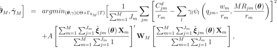
P C(qjm,wjm, M Rjm(θ0)) =

∞

X

l=1

γlψl(qjm,wjm, M Rjm(θ0)), (22)

where ψ1(·), ψ2(·), . . . are the basis functions for the sieve and γ1, γ2, . . . is a sequence of

their coefficients, satisfying P∞

l=1γ 2

l <∞.18

18_{Suppose the vector (q}