The permutation classes
Av(1234
,
2341) and Av(1243
,
2314)
David Bevan
Department of Mathematics and Statistics The Open University
Milton Keynes England
Abstract
We investigate the structure of the two permutation classes defined by the sets of forbidden patterns {1234,2341} and {1243,2314}. By consid-ering how the Hasse graphs of permutations in these classes can be built from a sequence of rooted source graphs, we determine their algebraic generating functions. Our approach is similar to that of “adding a slice”, used previously to enumerate various classes of polyominoes and other combinatorial structures. To solve the relevant functional equations, we make extensive use of the kernel method.
1
Introduction
We consider a permutation to be simply an arrangement of the numbers 1,2, . . . n for some positiven. A permutationπ is said to becontained in another permutation
σ if σ has a subsequence whose terms have the same relative ordering as those of
π. For example, 3241 is contained in 1573462 because the subsequence 5362 is ordered in the same way as 3241. If π is not contained in σ then we say that σ avoids π. For example, 1573462 avoids 3214. In the context of containment and avoidance, a permutation is often called a pattern.
The containment relation is a partial order on the set of all permutations, and a set of permutations closed downwards (a down-set) in this partial order is called a permutation class. It is natural to define a permutation class by the minimal set of permutations that it avoids. This minimal forbidden set of patterns is known as the basis of the class. The class with basis B is denoted Av(B).
Given a permutation class C, we denote by Cn the set of permutations in C of lengthn. The (univariate) generating function ofC is thenn1|Cn|zn=σ∈Cz|σ|, where|σ|is the length of σ. Thegrowth rate of C is defined by the limit lim
n→∞
n
if it exists. It is widely believed (see the first conjecture in [9]) that all permutation classes have a growth rate.
In the study of permutation classes, there has been significant interest in deriving the generating functions for classes with a few small basis elements (see [10] for an up-to-date list of results). This has led to the enrichment of the theory of permutation classes due to the requisite development of a variety of enumeration techniques. We add to this work by proving the following two theorems:
Theorem 1.1 The class of permutations avoiding1234 and 2341 has the algebraic generating function
2−10z+ 9z2+ 7z3−4z4 − (2−8z+ 9z2−3z3)√1−4z (1−3z+z2)(1−5z+ 4z2) + (1−3z)√1−4z .
Its growth rate is equal to 4.
Theorem 1.2 The class of permutations avoiding 1243 and2314 has an algebraic generating function F(z) which satisfies the cubic polynomial equation
(z−3z2+ 2z3)− (1−5z+ 8z2−5z3)F(z) + (2z−5z2+ 4z3)F(z)2 +z3F(z)3 = 0.
Its growth rate is approximately 5.1955, the greatest real root of the quintic polynomial
2−41z+ 101z2−97z3 + 36z4−4z5.
1.1 Hasse graphs
Corresponding to each permutation σ, we define an ordered plane graph Hσ, which we call itsHasse graph. IfPσ is the poset on the points (i, σi) in which (i, σi)<(j, σj) if bothi < jandσi < σj, thenHσ is the graph corresponding to the Hasse diagram of
Pσ. See the figures throughout this paper for illustrations showing the Hasse graphs of permutations. In practice, we tend not to distinguish between a permutation and its Hasse graph. The minimal elements of the poset Pσ are known as the left-to-right minima of the permutation σ. Similarly, maximal elements of Pσ are called right-to-left maxima of σ.
Hasse graphs of permutations were previously considered by Bousquet-M´elou & Butler [4], who determined the algebraic generating function of the family of forest-like permutations whose Hasse graphs are acyclic. More recently, they have been used by the present author [2] to establish a new lower bound for the growth rate of
Av(1324).
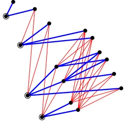
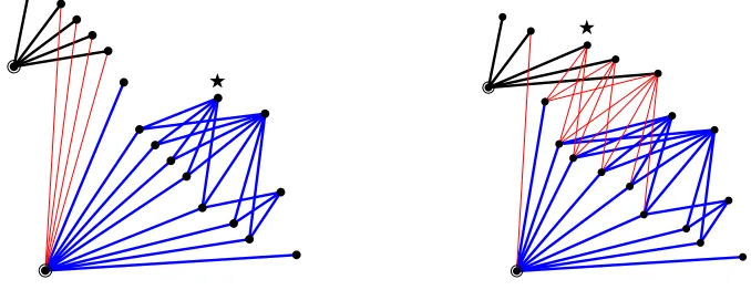
Given a permutation σ, we partition the vertices of Hσ by spanning it with a sequence of graphs, which we call the source graphs of σ. There is one source graph for each left-to-right minimum ofσ. Suppose u1, . . . , um are the vertices ofHσ corresponding to the left-to-right minima of σ, listed from left to right. Then the
and to the right of uk that are not in G1, . . . , Gk−1. We refer to uk as the root of source graphGk. See Figure 1 for an illustration. The structure of the source graphs of permutations in a specific permutation class is constrained by the need to avoid the patterns in the basis of the class. If the source graphs for some class are acyclic, we refer to them as source trees.
The bottom subgraph of a Hasse graph is the graph induced by its lowest vertex (the least entry in the permutation) and all the vertices lying above and to its right. Observe that the bottom subgraph may contain vertices from more than one source graph. For example, the bottom subgraph of the Hasse graph in Figure 1 contains vertices from three source graphs. Bottom subgraphs of permutations in a specific permutation class satisfy the same structural restrictions as do the source graphs. We refer to an acyclic bottom subgraph as a bottom subtree.
We build the Hasse graph of a permutation by starting with a source graph and then repeatedly adding another source graph to the lower right. The technique is sim-ilar to that of “adding a slice”, which has been used to enumerate constrained com-positions and other classes of polyominoes, a topic of interest in statistical mechanics (see, for example, Bousquet-M´elou’s review paper [3], the books of van Rensburg [8] and Guttmann [6], and Flajolet & Sedgewick [5, Examples III.22 and V.20]). When a source graph is added, its vertices are interleaved horizontally with the non-root vertices of the bottom subgraph of the graph built from the previous source graphs. Typically, the positioning of the vertices of the new source graph is constrained by the need to avoid forbidden patterns.
In order to derive the univariate generating functions we require, we make use of multivariate functions involving additional “catalytic” variables that record certain parameters of the bottom subgraph of the permutations. These additional variables enable us to establish recurrence relations which we can then solve using the kernel method. Typically, when employing a multivariate generating function, we treat it simply as a function of the relevant catalytic variable, writing, for example, F(u) rather than F(z, u).
Occasionally, we also make use of a variant of the symbolic structural notation presented in Flajolet & Sedgewick [5] to establish functional equations. In particular,
Z is the atomic class consisting of a single vertex, and we use Seq[A] to represent a possibly empty sequence of elements of A and Seq+[A] to represent a non-empty sequence of elements ofA.
The two classes we enumerate are quite distinct structurally. A source graph in
Av(1234,2341) consists of a root together with a123-avoider formed from the non-root vertices. However, the presence of a 123forces any subsequent source graph to be simply a fan. In contrast, Av(1243,2314) has plane source graphs and a much more uniform structure. We enumerateAv(1234,2341) in Section 2. In doing so, the kernel method is used six times to solve the relevant functional equations. The class
Figure 1: A permutation in class F, spanned by four source graphs
2
Permutations avoiding 1234 and 2341
Let us use F to denoteAv(1234,2341). The structure of class F depends critically on the presence or absence of occurrences of the pattern 123. In light of this, to enumerate this class, we partition it into three sets A, B and C as follows:
• A=Av(123).
• B =Av(1234,2341,13524,14523)\ A. Every permutation in B contains at least one occurrence of a 123, but avoids 13524 and 14523.
• C =Av(1234,2341)\(A ∪ B). Every permutation inC contains a 13524 or a
14523.
We refer to a permutation in A as an A-permutation, and similarly for B and C.
The addition of a source graph to aC-permutation can only yield another permu-tation in C (since it can’t cause the removal a 13524 or 14523 pattern). Similarly, the addition of a source graph to aB-permutation can’t result in anA-permutation. Hence, we can enumerate A without first considering B orC, and can enumerate B before considering C.
Before investigating the structure of permutations in A, B and C, let us briefly examine what a typical source graph in F looks like. Firstly, the avoidance of 1234
means that the non-root vertices of any source graph form a123-avoider. Secondly, the avoidance of2341 presents no additional restriction on the structure of a source graph, because the presence of a2341would imply the presence of a123 in the non-root vertices. Thus a source graph inF consists of a root together with a123-avoider formed from the non-root vertices.
2.1 The structure of set A
Figure 2: Adding a source tree to the bottom subtree of an A-permutation
Let AS denote the set of source graphs in set A. Now, each member of AS is simply a fan, a root vertex connected to a (possibly empty) sequence of pendant edges. Bottom subgraphs are also fans. Thus source graphs and bottom subgraphs of A are acyclic.
When enumerating A, we use the variableu to mark thenumber of leaves (non-root vertices) in the bottom subtree. The generating function for AS is thus given by
AS(u) = z+z2u+z3u2+. . . = 1−zzu.
We now consider the process of building an A-permutation from a sequence of source trees. When a source tree is added to an A-permutation, the root vertex of the source tree may be inserted to the left of zero or more of the leaves of the bottom subtree. See Figure 2 for an illustration. Note that, in this and other similar figures, the original bottom subgraph is displayed to the upper left, with the new source graph to the lower right.
The action of adding a source tree is thus seen to be reflected by the linear operator ΩA whose effect on uk is given by
ΩAuk = AS(u)(1 +u+. . .+uk) = AS(u)1−u
k+1
1−u .
Hence, the bivariate generating function A(u) for A is defined by the following re-cursive functional equation:
A(u) = AS(u) + AS(u)A(1)−uA(u) 1−u .
This equation can be solved using the kernel method. To start, we express A(u) in terms of A(1), by expanding and rearranging to give
A(u) = z
1−u+A(1)
1−u+zu2 . (2.1)
Equivalently, we have the equation
(1−u+zu2)A(u) = z1−u+A(1).
the kernel). The appropriate root to use can be identified from the combinatorial requirement that the series expansion of A(1) contains no negative exponents and has only non-negative coefficients.
In this case, the correct root is u= (1−√1−4z)/2z, which yields the univariate generating function forA,
A(1) = 1−
√
1−4z 2z −1.
This is the generating function for the Catalan numbers as expected.
Finally, by substituting for A(1) back into (2.1) we get the following explicit algebraic expression forA(u):
A(u) = 1−2zu−
√
1−4z 2(1−u+zu2) .
On this occasion, we have explained every step of the derivation. On subsequent occasions, we present fewer details of the algebraic manipulations.
[image:6.595.255.360.369.478.2]
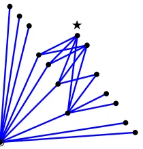
Figure 3: A source graph in set B
2.2 The structure of set B
We now consider set B. Recall that sets B and C consist of those permutations in class F that contain at least one occurrence of a 123. We need to keep track of the position of the leftmost occurrence of a 3in such a pattern. Given a permutation in
B or C, let us call the vertex corresponding to the leftmost 3 in a 123 the spike. In the figures, the spike is marked with a star.
We now make a key observation. When adding a source graph to a permutation containing a 123, no vertex of the source graph may be positioned to the right of the spike, or else a 2341 would be created. Hence, the spike in any permutation in classes B orC occurs in its bottom subgraph. When enumerating sets B and C, we use the variableuto markthe number of vertices to the left of the spike in its bottom subgraph.
LetBS be the set of source graphs in setB. Since B-permutations contain a 123
two descending sequences, the second sequence beginning (with the spike) above the last vertex in the first sequence. See Figure 3 for an illustration. If we consider the non-root vertices in order from top to bottom, then it can be seen that BS is defined by the structural equation
BS = uZ × Seq[uZ] × Z × Seq[uZ +Z] × uZ × Seq[Z].
The first term on the right corresponds to the root and the remaining terms deal with the non-root vertices in order from top to bottom, vertices to the left of the spike being marked with u. The third term corresponds to the spike and the fifth represents the lowest point to the left of the spike (the rightmost2of a123). Hence, the generating function forBS is
BS(u) = z
3u2
(1−z)(1−zu)(1−z−zu).
We now study the process of building aB-permutation from a sequence of source graphs. There are two cases. A permutation inBmay result either from the addition of a source graph to anA-permutation, or else from adding a source graph to another
B-permutation. We address these two cases in turn.
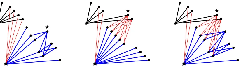
[image:7.595.103.516.403.526.2]
Figure 4: Ways to create aB-permutation by adding a source graph to the bottom subtree of an A-permutation
One way to create a B-permutation from an A-permutation is to add a source graph from BS, positioning its root to the left of zero or more of the leaves of the bottom subtree of the A-permutation and its non-root vertices to the right of the bottom subtree. In this case, the new permutation inherits its spike from the added source graph. This is illustrated in the left diagram in Figure 4. The generating function for this set of permutations is thus given by
BAB1(u) = BS(u)A(1)−uA(u)
1−u .
The other possibility for creating a B-permutation from an A-permutation in-volves the positioning of some non-root vertices of the source graph to the left of some of the leaves in the bottom subtree, making one of the vertices in the original bottom subtree the spike. The source graph may be drawn from either AS or BS, as illustrated in the centre and right diagrams in Figure 4.
In this situation, if the source graph has a spike, it must be positioned to the right of all leaves in the bottom subtree, or else a 1234 would be created. Furthermore, any source graph vertices placed to the left of leaves in the bottom subtree must occur at the same position in the bottom subtree, or else a13524 would be created. This position may be chosen independently of where the root vertex is placed.
From these considerations, it can be determined that the resulting set of permu-tations has the generating function defined by
BAB2(u) =
BS(u) + z
2u2
(1−z)(1−zu) 1 1−u
A(1)− u
1−u
A(1)−A(u) ,
where the presence of the derivative A is a consequence of the independent choice of two positions in the bottom tree.
[image:8.595.262.346.384.472.2]
Figure 5: Adding a source tree to the bottom subgraph of aB-permutation
Finally, we consider the addition of a source graph to a B-permutation. As we noted in our key observation on page 8, no vertex of the source graph may be positioned to the right of the spike in the bottom subgraph. As a result, the new source graph may not contain a123 or else a 1234 would be created, so the source graph must be a member ofAS (a fan). Moreover, the leaves of the source tree must be positioned immediately to the left of the spike, or else a 1234 would be created. See Figure 5 for an illustration.
Note that, as a consequence of these restrictions, it is impossible for the addition of a source graph to a B-permutation to create a 13524 or 14523. So it is not possible to extend a B-permutation so as to create a C-permutation.
Thus the bivariate generating function B(u) of set B is defined by the following recursive functional equation:
B(u) = BS(u) +BAB1(u) +BAB2(u) + zu 1−zu
B(1)−B(u) 1−u ,
This equation is amenable to the kernel method. After rearrangement to express
B(u) in terms ofB(1), the kernel can be cancelled by setting u= (1−√1−4z)/2z, which yields the following expression forB(1):
B(1) = −1 + 8z−19z
2+ 12z3 + (1−6z+ 9z2−2z3)√1−4z
2z3(1−4z) .
Substitution then results in an explicit algebraic expression forB(u), which we refrain from presenting explicitly due to its size.
Figure 6: A source graph in set C
2.3 The structure of set C
We begin our enumeration ofC by counting its set of source graphs, which we denote
CS. Rather than doing this directly, we enumerate all the source graphs that contain
a 123 (i.e. those in either BS or CS) and then subtract those in BS. To begin, we consider how we might build anarbitrary source graph in classF by adding vertices from left to right.
Suppose we have a partly formed source graph with at least one non-root vertex, whose rightmost vertex isv, and we want to add further vertices to its right. What are the options? Ifv is not the lowest of the non-root vertices, then any subsequent vertices must be placed lower thanv. The only other restriction is that vertices must be positioned higher than the root. If we use y to mark the number of positions in which a vertex may be inserted, then the action of adding a new vertex can be seen to be reflected by the following linear operator:
ΩLf(y) = zy2f(1)−f(y) 1−y .
We choose to denote this operator ΩL because it corresponds to the action used in building a Lukasiewicz path.
to the left of the spike. If, in addition, we mark withy those vertices not above the spike, then BS0 is defined by the structural equation
BS0 = uZ × Seq[uZ] × Seq+[uyZ] × yZ.
It is readily seen thatycorrectly marks the number of positions in which an additional vertex may be inserted to the right.
Let DS = BS∪ CS. Since every member of DS is built from an element of BS0 by applying ΩL zero or more times, it follows that the generating function for DS is defined by the recursive functional equation
DS(y) = z
3y2u2
(1−zu)(1−zyu) + zy
2DS(1)−DS(y)
1−y .
This equation can be solved for DS(1) by utilising the kernel method, setting y = (1−√1−4z)/2z to cancel the kernel. The generating function forCS is then defined by
CS(u) = DS(1) − BS(u).
We now study the process of building a C-permutation from a sequence of source graphs. As with set B, there are two cases. A permutation in C may result either from the addition of a source graph to an A-permutation, or else from adding a source graph to another C-permutation. (As we observed above, it is not possible to create a C-permutation by adding a source graph to a B-permutation.) We address the two cases in turn.
[image:10.595.134.473.465.596.2]
Figure 7: Ways to create a C-permutation by adding a source graph to the bottom subtree of an A-permutation
One way to create a C-permutation from an A-permutation is to add a source graph from CS, positioning its root to the left of zero or more of the leaves of the bottom subtree of the A-permutation and its non-root vertices to the right of the bottom subtree. This is illustrated in the left diagram in Figure 7. The generating function for this set of permutations is thus
CAC1(u) = CS(u)A(1)−uA(u)
The other method for creating a C-permutation from an A-permutation involves the positioning of some non-root vertices of the source graph to the left of some of the leaves in the bottom subtree. This is illustrated in the right diagram in Figure 7. In analysing this method, it is more convenient to look, more generally, at how an
A-permutation can be extended to yield a permutation containing a 123, in either
B or C. We can then subtract those members of B that are enumerated by BAB2. We achieve the enumeration by adding vertices from left to right in four steps:
1. The first step adds the root.
2. The second step adds the first non-root vertex, which determines the position of the new spike, and also any other vertices positioned to the left of the spike.
3. The third step adds any additional vertices to the right of the spike but to the left of some other leaves in the bottom subtree. The addition of such vertices creates occurrences of 13524.
4. Finally, the fourth step adds any vertices to the right of the bottom subtree.
Step 1: Permutations that result from the addition of the root vertex are enu-merated by
D1(u) = zuA(1)1−−Au(u).
Step 2: In this step, we insert the descending sequence of vertices that creates the new spike. In the generating function for permutations resulting from this action, we introduce two additional catalytic variables that we require for steps 3 and 4. For use in step 3,v marks the number of source tree leaves to the right of the new spike. For step 4, we use y to mark valid positions for the insertion of subsequent vertices, as we did previously. The generating function is
D2(v) = zy
2u2
1−zyu
D1(v)−D1(u)
v−u .
Step 3: The effect of adding additional vertices to the right of the spike but to the left of some other leaves in the bottom subtree is represented by the recursive functional equation
D3(y, v) = D2(v) + zyvD3(y,1)1−−Dv 3(y, v).
Again, the kernel method can be used to solve this for D3(y,1), the kernel being cancelled by setting v = 1/(1−zy).
Step 4: Finally, the addition of vertices to the right of the bottom subtree is reflected by the Lukasiewicz operator ΩL, giving rise to the recursive functional equation
D4(y) = D3(y,1) + zy2D4(1)1−−Dy 4(y),
The generating function for the set of permutations resulting from the second way of creating a C-permutation from an A-permutation is then defined by
CAC2(u) = D4(1)−BAB2(u).
Our work is almost complete. We only have to consider how a source graph may be added to a C-permutation. In fact, the situation is extremely constrained. First, as noted earlier, the source graph must be positioned to the left of the spike. Furthermore, the presence of a13524 or14523 means that the addition of a source graph with even a single non-root vertex would create a1234. So the only possibility is the addition of a trivial (single vertex) source tree. Thus the bivariate generating function C(u) of setC is defined by the following recursive functional equation:
C(u) = CS(u) +CAC1(u) +CAC2(u) + zuC(1)−C(u) 1−u .
where the final term reflects the addition of a trivial source tree to a C-permutation. This equation can be solved to yield the following expression forC(1) by a sixth and final application of the kernel method, cancelling the kernel by settingu = 1/(1−z):
C(1) = P(z) + Q(z)
√
1−4z 2z3(1−4z)(1−3z+z2),
where
P(z) = −1 + 10z−35z2+ 52z3−35z4+ 12z5,
Q(z) = 1− 8z+ 21z2−22z3+ 11z4− 2z5.
We now have all we need to prove Theorem 1.1 by obtaining an explicit expression for the generating function that enumerates class F. Since F is the disjoint union of A, B and C, its generating function is given by A(1) +B(1) +C(1). Thus, by appropriate expansion and simplification, the generating function forAv(1234,2341) can be shown to be equal to
2−10z+ 9z2+ 7z3−4z4 − (2−8z+ 9z2−3z3)√1−4z (1−3z+z2)(1−5z+ 4z2) + (1−3z)√1−4z .
This has singularities atz = 14,z = 12(3−√5) andz = 12(3 +√5). Hence, the growth rate of Av(1234,2341) is equal to 4, the reciprocal of the least of these.
The first twelve terms of the sequence |Fn| are 1, 2, 6, 22, 89, 376, 1611, 6901, 29375, 123996, 518971, 2155145. More values can be found at A165540 in OEIS [7].
3
Permutations avoiding 1243 and 2314
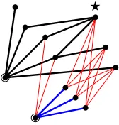
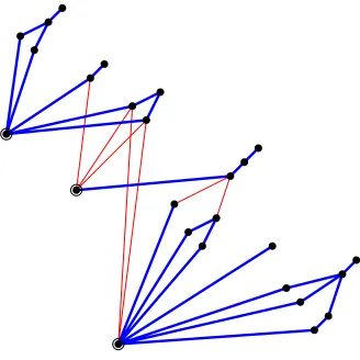
Figure 8: A permutation in class E, spanned by three source graphs
root of a source graph may fork towards the upper right. Secondly, each source graph inE isplane. This is the case because every non-plane graph contains aH2143 = , and, furthermore, any2143in a source graph occurs as part of a13254(where the1
is the root of the source graph). But this is impossible in E, since 13254 does not avoid 1243.
Figure 9: A source graph for class E, constructed from four u-trees
If we combine these two observations, we see that the non-root vertices of a source graph consist of a sequence of inverted subtrees whose roots are right-to-left maxima. The avoidance of H2314 = places restrictions on the structure of the subtrees, so that they must consist of a path at the lower right, which we call the trunk, with pendant edges attached to its left. It is readily seen that these correspond to permutations inAv(132,231). We call trees of this formu-trees, short forunbalanced trees. See Figure 9 for an illustration of a source graph constructed from u-trees.
The class U of u-trees satisfies the structural equation
U = Z ×Seq[Z ×Seq[Z]]
[image:13.595.240.372.399.529.2](possibly empty) sequence of pendant edges attached to the upper left. Hence the generating function forU is
U(z) = z(1−z) 1−2z .
If we use u to mark the number of u-trees, the class S of source graphs satisfies the structural equation
S = Z ×Seq[uU] and thus has bivariate generating function
S(u) = S(z, u) = z(1−2z) 1−(2 +u)z+uz2.
[image:14.595.124.496.375.539.2]Let us now examine how a permutation in E can be built from a sequence of source graphs. Observe that, when a source graph is added, no vertex of the source graph can be positioned between two vertices of a u-tree in the bottom subgraph, because otherwise a2314would be created. In addition, there are strong constraints on when u-trees in the new source graph can be positioned to the left of a u-tree in the bottom subgraph.
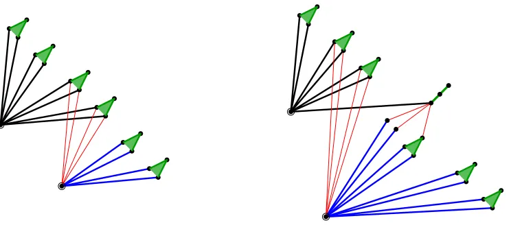
Figure 10: The two methods for adding a source graph in class E; u-trees are shown schematically as filled triangles
These conditions result in there being two distinct ways in which a source graph may be added. These are illustrated in Figure 10. In the first method, the root of the source graph is positioned to the left of zero or more u-trees in the bottom subgraph and the u-trees in the source graph are positioned to the right of the bottom subgraph.
In order to handle this second method, we need to keep track of those source graphs in which the rightmost u-tree is a path. Let SP be the class of such graphs. It satisfies the structural equation
SP = Z ×Seq[uU]×uSeq+[Z],
where umarks the number of u-trees as before. This class thus has bivariate gener-ating function
SP(u) = SP(z, u) = uz
2(1−2z)
(1−z)1−(2 +u)z+uz2.
In order to distinguish between those situations when the second method of adding a source graph is applicable and those when it isn’t, let us use P to de-note the set of those permutations inE whose Hasse graphs have bottom subgraphs in which the rightmost u-tree is a path.
We are interested in determining the two bivariate generating functions E(u) =
E(z, u) and P(u) =P(z, u) for E and P respectively, where u marks the number of u-treesin the bottom subgraph. To do this, we will establish four linear operators on these generating functions that reflect the different ways in which a source graph can be added.
The action of adding a source graph using the first method is readily seen to be reflected by the following linear operator:
ΩEEf(u) = S(u)f(1)−uf(u) 1−u .
The first method creates a member of P from an arbitrary element of E whenever the source graph is in SP (i.e. its rightmost u-tree is a path). Thus the appropriate linear operator is
ΩEPf(u) = SP(u)f(1)−uf(u) 1−u .
Now let us determine the linear operators corresponding to the second method of adding a source graph.
The set, S, of source graphs that can be added using the second method satisfies the structural equation
S = Z ×
Seq[Z]×uU ×Seq[uU],
in which the third term on the right identifies the u-tree which is positioned im-mediately to the left of the rightmost (path) u-tree in the bottom subgraph. This specification thus counts multiple times those source graphs that can be added in more than one way due to the presence of a non-empty initial sequence of single-vertex u-trees. Note also that we don’t mark the initial sequence of single-single-vertex u-trees with u. The generating function for S is
S(u) = uz2
The action of adding a source graph using the second method is then seen to be reflected by the following linear operator:
ΩPEfP(u) = S(u)fP(1)−fP(u) 1−u .
Finally, let us consider when adding a source graph to an arbitrary member of P creates another permutation in P. The second method creates an element of P if the source graph is in SP and its rightmost (path) u-tree is added to the right of the bottom subgraph. An element of P is also created if the source graph has a single path u-tree or consists of a single vertex (the root). Thus the set, SP, of source graphs, counted with multiplicity, that can be added to create an element of
P satisfies the structural equation
S
P = Z ×Seq[Z]×Seq+[uU]×uSeq+[Z] + Z ×uSeq[Z].
Its generating function is
S
P(u) = uz
(1−2z)(1−uz) (1−z)1−(2 +u)z+uz2,
and the corresponding linear operator is
ΩPPfP(u) = SP(u)fP(1)−fP(u) 1−u .
We are now in a position to derive the generating function for E and hence prove Theorem 1.2. From the analysis above, we know that the bivariate generating function E(u) = E(z, u) of class E is defined by the following pair of mutually recursive functional equations:
E(u) = S(u) + ΩEEE(u) + ΩPEP(u)
P(u) = SP(u) + ΩEPE(u) + ΩPPP(u) .
These can be expanded to give the following:
E(u) = z(1−2z)
1−u+E(1)−uE(u) + uzP(1)−P(u)
(1−u)1−(2 +u)z+uz2 , (3.1)
P(u) = uz(1−2z)z
1−u+E(1)−uE(u) + (1−uz)P(1)−P(u)
(1−u)(1−z)1−(2 +u)z+uz2 . (3.2)
An unusual simultaneous double application of the kernel method can then be used to yield the algebraic generating function for class E as follows.
First, we eliminate P(u) from (3.1) and (3.2), and express E(u) in terms ofE(1) and P(1) as a rational function. Cancelling the resulting kernel,
with the appropriate root then gives us an equation relating E(1) and P(1).
Secondly, we eliminate E(u) from (3.1) and (3.2), and express P(u) in terms of
E(1) and P(1). Cancelling the (same) kernel (using a different root) gives a second equation relating E(1) andP(1).
Finally, we eliminate P(1) from these two equations to yield an extremely com-plicated explicit expression for E(1).
Thus, using a computer algebra system to handle the details of the algebraic manipulation, it can be determined that the generating function F(z) = E(1) for
Av(1243,2314) has the minimal polynomial
(z−3z2+ 2z3) − (1−5z+ 8z2−5z3)F(z) + (2z−5z2+ 4z3)F(z)2 + z3F(z)3.
The growth rate of the class is given by the reciprocal of the least positive real singu-larity of its generating function [5, Theorems IV.6 and IV.7]. Hence, by determining the location of the singularities ofE(1), it is possible to establish that the growth rate of class E is approximately 5.1955, the greatest real root of the quintic polynomial
2−41z+ 101z2−97z3 + 36z4−4z5,
as required.
The first twelve terms of the sequence |En| are 1, 2, 6, 22, 88, 367, 1571, 6861, 30468, 137229, 625573, 2881230. More values can be found at A165539 in OEIS [7].
Acknowledgements
Michael Albert’s PermLab software [1] was of particular benefit in helping to visualise and explore the structure of permutations in the two permutation classes. The author is also grateful to Robert Brignall and two anonymous referees for suggestions that led to improvements in the presentation of parts of the paper.
Soli Deo gloria!
References
[1] Michael Albert, PermLab: Software for permutation patterns, http://www.cs .otago.ac.nz/PermLab, 2012.
[2] David Bevan, Permutations avoiding 1324 and patterns in Lukasiewicz paths, J. London Math. Soc. 92 (1) (2015), 105–122.
[3] Mireille Bousquet-M´elou, A method for the enumeration of various classes of column-convex polygons, Discrete Math. 154 (1996), 1–25.
[5] Philippe Flajolet and Robert Sedgewick, Analytic Combinatorics, Cambridge University Press, 2009.
[6] Anthony J. Guttmann, editor, Polygons, Polyominoes and Polycubes, Lecture Notes in Physics Vol. 775, Springer, 2009.
[7] The OEIS Foundation Inc, The On-Line Encyclopedia of Integer Sequences, published electronically athttps://oeis.org.
[8] E. J. Janse van Rensburg, The Statistical Mechanics of Interacting Walks, Poly-gons, Animals and Vesicles, vol. 18 ofOxford Lecture Series in Mathematics and its Applications, Oxford University Press, 2000.
[9] Vincent Vatter, Permutation classes, In Mikl´os B´ona (ed.), The Handbook of Enumerative Combinatorics, CRC Press, 2015.
[10] Wikipedia, Enumerations of specific permutation classes,http://en.wikipedia .org/wiki/Enumerations of specific permutation classes.