Fauxvea: Crowdsourcing Gaze Location Estimates for Visualization Analysis Tasks

(1)

City, University of London Institutional Repository

Citation

:

Gomez, S., Jianu, R., Cabeen, R., Guo, H. & Laidlaw, D. H. (2016). Fauxvea:

Crowdsourcing Gaze Location Estimates for Visualization Analysis Tasks. IEEE Transactions

on Visualization and Computer Graphics, doi: 10.1109/TVCG.2016.2532331

This is the accepted version of the paper.

This version of the publication may differ from the final published

version.

Permanent repository link: http://openaccess.city.ac.uk/15398/

Link to published version

:

http://dx.doi.org/10.1109/TVCG.2016.2532331

Copyright and reuse:

City Research Online aims to make research

outputs of City, University of London available to a wider audience.

Copyright and Moral Rights remain with the author(s) and/or copyright

holders. URLs from City Research Online may be freely distributed and

linked to.

(2)

Fauxvea: Crowdsourcing Gaze Estimates for

Visualization Analysis Tasks

Abstract—We present the design and evaluation of a method for estimating gazes during the analysis of static visualizations using crowdsourcing. Understanding gaze patterns is helpful for evaluating visualizations and user behaviors, but traditional eye-tracking studies require specialized hardware and local users. To avoid these constraints, we created a method called Fauxvea, which crowdsources visualization tasks on the Web and estimates gaze fixations through cursor interactions without eye-tracking hardware. We ran experiments to evaluate how gaze estimates from our method compare with eye-tracking data. First, we evaluated crowdsourced estimates for three common types of information visualizations and basic visualization tasks using Amazon Mechanical Turk (MTurk). In another, we reproduced findings from a previous eye-tracking study on tree layouts using our method on MTurk. Results from these experiments show that fixation estimates using Fauxvea are qualitatively and quantitatively similar to eye tracking on the same stimulus-task pairs. These findings suggest that crowdsourcing visual analysis tasks with static information visualizations could be a viable alternative to traditional eye-tracking studies for visualization research and design.

Index Terms—Eye tracking, crowdsourcing, focus window, information visualization, visual analysis, user studies

F

1 I

NTRODUCTION

T

HEgoal of this work is to make it easier to understand

where people look in visualizations during analysis tasks. This gaze information is helpful for improving vi-sualization designs. For example, gaze data can reveal whether users attend to guide marks in a visualization. A potential application is verifying that increasing the size of marks or repositioning them draws attention to them, thus helping people interpret the visualization. Finding where people look can also help researchers understand analysis strategies and might improve their ability to identify low-level analysis activities, like finding extrema in a chart [1]. Ultimately, this information could be used to improve the usability of visualization interfaces or choose more effective visual mappings for data visualizations.

We present an evaluation of a crowd-based method for estimating gaze fixations for visualizations. The method builds on an earlier technique called the Restricted Focus Viewer (RFV) [2], an image viewer that simulates move-ment of the fovea by blurring the image and requiring viewers to deblur regions using the cursor. Essentially, the RFV requires a person to make manual interactions that are easily recorded and correspond the areas of the image she wants to visually decode. We constructed a Web-based version of the RFV called Fauxvea, which has incremental improvements in the design of the focus window and data capture, but most importantly can be accessed by remote study participants like crowd workers. As a result, the method enables large-scale gaze estimation experiments, and can be used to crowdsource the production of heatmaps showing gaze for visualization stimulus-task pairs.

We demonstrate the method using workers on Amazon Mechanical Turk (MTurk). First, we compared Fauxvea fix-ation estimates to eye tracking from 18 participants for three

common types of information visualization (infovis) charts – scatter plots, bar charts, and node-link diagrams – plus photographs. Second, we compared the Fauxvea estimates with ones predicted by participants with expertise in vision and eye tracking; we show that an individual, even one with experience with vision, cannot predict fixations as well as data from a study using Fauxvea. Third, we reproduced findings from an existing study on tree layouts from Burch et al. [3] that involves a more complex visual analysis task than in the first experiment. In these experiments, we find that gaze locations on the visualizations by online participants are qualitatively and quantitatively similar to gazes from the eye-tracking study.

The contributions of this work are fourfold:

• a novel method for crowdsourcing gaze fixation

esti-mates for visualization analysis tasks (Sec. 3);

• qualitative and quantitative evaluations of the method

that show fixation estimates are comparable to eye-tracking data on basic infovis analysis tasks (Sec. 4);

• an evaluation of how well experts can self-assess

where others will gaze during visualization analysis tasks; we compare self-assessment to data collected using Fauxvea (Sec. 5);

• reproduced findings about visual exploration on tree

layouts using the method instead of eye tracking for a more complex graph analysis task (Sec. 6).

Finally, we discuss limitations of the method and present opportunities for developing models of gaze that factor in both visualization stimuli and analysis tasks.

2 R

ELATED

W

ORK

(3)

IEEE TRANSACTIONS ON VISUALIZATION AND COMPUTER GRAPHICS 2

2.1 Focus-Window Methods

The idea of restricting visual information to the location of a pointer and tracking its location has existed for decades. An early example is the MOUSELAB system, which was aimed at tracking a study participant’s cognitive process during decision tasks involving information on a computer display [4]. In this system, boxes containing information appeared blank until the participant moved the mouse into one, which would reveal the information in that box.

Our method is more closely related to the Restricted Focus Viewer (RFV) [2], an image viewer that requires the user to move the cursor in order to focus regions of the image. Unlike MOUSELAB, the RFV works with images that do not have predefined boundaries of information, so the mouse can be moved to focus any part of the image, and the image outside of the focus window is blurred. Cursor movements can be recorded and replayed as a proxy for actual gaze fixations. Fauxvea adapts this technique for the Web browser, with design changes that make it easier to use. Most significantly, the experiments we performed demonstrate that gaze estimates collected from online crowd workers – even in uncontrolled computing en-vironments – are close to eye tracking for the visualization tasks we studied.

Previous evaluations of the RFV in controlled laboratory experiments have validated the technique and identified some of its limitations, but to the best of our knowledge we are the first to explore its use in estimating gaze during analysis tasks with data visualizations. Blackwell et al. found that when people evaluated causal motions in diagrams of pulley systems, gaze patterns estimated by the RFV were similar to patterns collected from an eye-tracking study on the same stimuli [2]. Bednarik and Tukiaine [5] studied how participants in a controlled eye-tracking study used a Java software debugging environment with the RFV. They found that blurring affected how some users switched gaze between areas on the screen differently compared to eye tracking, but this behavior did not affect task performance; participants were able to extract the same information using the RFV as with a normal image viewer. Stimuli like coding environments or pulley diagrams differ from typical infovis charts in how directly they encode information, so we are motivated to study the focus-window method in this context. We find supporting evidence that the approach works even in realistic visualization scenarios involving moderately complex visual representations and tasks. For instance, as described in Sec. 6.3, we found similarities between eye tracking and our crowd-powered RFV (Fauxvea) in how people switched between areas of interest in tree diagrams during a graph analysis task.

Crowdsourcing might also help users of the RFV to select appropriate parameters for their experiments. Jones and Mewhort [6] found that badly chosen blur levels outside the focus window can affect scan patterns. Earlier works have proposed guidelines for setting blur levels [2], [7], but it remains a challenge to apply these. Because picking blur parameters depends on the stimulus-task and not on

individual differences, blur levels for stimuli and tasks could be tested rapidly, inexpensively, and at scale in pilot studies on MTurk. In our experiment, we chose a reasonable blur level after rapid testing on MTurk.

2.2 Estimating Gaze on the Web

User interfaces have been developed to collect gaze es-timates using a Web browser, but these have focused on domains outside of visualization. Much of this work is based on findings about the relationship between gaze and cursor movements (e.g., [8]), which are easy to track in Web applications. Other studies using Web search tasks in lab settings have identified specific types of eye-mouse coor-dination patterns [9], [10] and demonstrated the predictive power of cursor actions for estimating gaze [11]. Huang et al. performed an eye-tracking study relating cursor activity to gaze in search engine results pages (SERPs), then followed up with a large-scale study of cursor tracking that linked cursor movements and results examination behaviors in SERPs [12]. Our method also uses cursor actions to predict gaze, but we make use of deliberate cursor presses and releases rather than hover locations in order to measure start and end times for gaze fixations.

A Web-based system related to a moving focus window is ViewSer, which helped researchers study how remote users examine SERPs without eye-tracking [13]. The in-terface blurs DOM elements in the page corresponding to search results, and deblurs results when users hover over them with the cursor. One limitation of this method for evaluating visualization analysis is that it can only deblur entire DOM elements. Even if visualization components do correspond with DOM elements, e.g., using D3 [14], the size of the the deblurred component might be large enough that the hovered location does not reflect where the user is gazing at a useful level of precision. With Fauxvea, the deblurring area is based on a simple model of the human fovea. Because the focus region becomes more blurred away from its center, the user must press the cursor near the pixels she wants to see clearly. Therefore, the precision of Fauxvea for estimating gaze is linked to a parameter in the model and is not dependent on the way DOM elements are rendered.

(4)

(a) Browser interface for Fauxvea

r d

p

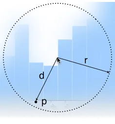
[image:4.567.344.462.52.179.2]

(b) Focus window during fixation

Fig. 1: Left: Fauxvea interface showing analysis task instructions, the blurred image viewer, and an input field for the task answer. This example shows a bar chart task from Experiment 1. Right: The focus window during a Fauxvea fixation.

All pixels outside radius r are fully blurred, and pixels inside are blended between the blurred image and the focused

one. The blend ratio for each pixel p is proportional to its distance d from the cursor location.

2.3 Crowdsourcing Visual Analysis Tasks

Recently, crowdsourcing platforms have been used to eval-uate visualizations with scalable, non-expert populations. Some notable examples include Heer and Bostock’s repro-duction of classic graphical perception results [16], Kong et al.’s study on TreeMap design [17], evaluations by Kosara and Ziemkiewicz of visual metaphors and percentage value reading [18], and Ziemkiewicz et al.’s study of the effects of individual differences on visualization performance [19]. This line of work has provided valuable examples and guidelines for crowdsourcing visualization analysis tasks, but they largely focus on evaluating the speed and accu-racy of Turkers’ task performance as outputs. Instead, we estimate gaze locations with Fauxvea using additional data from the task execution, e.g., cursor presses that facilitate performing a task.

3 D

ESIGN AND

M

ETHODS

We adapted the RFV into a Web-based application called Fauxvea that estimates gaze fixations during visualization analysis tasks without using eye-tracking hardware. By design, tasks on the interface can be performed in parallel by remote users, or crowdsourced as human intelligence tasks (HITs) on MTurk.

We had two main objectives when designing and building the Fauxvea prototype:

• Collect data that is comparable to eye tracking during

analysis of a static visualization.

• Enable scalable experiments with remote users, like

crowdsourced participants or remote domain experts who are unavailable for local eye-tracking studies.

3.1 Interface Design

Comparable to eye tracking–The goal of this work is to make gaze data and metrics more accessible to visualization designers and evaluators. We are mainly interested in the location and duration of fixations – where the eye is focused in the field of view and has the highest visual acuity. If we assume for simplicity the “eye-mind” hypothesis, this data

identifies areas of a visualization that a person cognitively processes during an analysis task.

No part of the Fauxvea viewer is focused until the user presses the cursor in the viewport. The time and location of each cursor press are recorded as the start time, end time, and location point of a fixation estimate. This is more precise than determining a fixation based on the speed of a hovering cursor, as in the original RFV. While the cursor is pressed, image details directly under the cursor are revealed within a focus radius, as shown in Figure 1. The blur approximates how details in one’s peripheral vision appear when the fovea is fixated elsewhere in the field of view; we use a radius instead of the original RFV’s rectangular window with steps of blur. The idea of a focus spotlight is similar to other approaches in foveated imaging and Focus+Context techniques in information visualization, like semantic depth of field [20]. We note that the information loss that occurs in peripheral vision and how it affects visual search are not fully understood. Others have argued that blur is too simple of a model and that other summary statistics may be computed over a pooling region in one’s vision [21]. Incorporating different models of lossy visual information into an RFV-like interface is an open challenge beyond the scope of this work.

For the experiments described later, the focus radius is

equal to the 1/6 the width of each stimulus, or 133 pixels.

For many desktop and laptop computing environments, we expect this radius is a reasonable approximation to the extent of the fovea, which is between 1–2 degrees of the field of view [22]. The Fauxvea focus region does not move if the user drags, forcing the user to release before pressing in a new location. This lets Fauxvea record fixation start and end times. The interface does not support zoom or pan operations, though scrolling in the browser window will not impact the interface. Within the focus radius, each pixel has a color that is a blend of corresponding colors in the original image and blurred image. The blend ratio for each pixel is proportional to its distance from the cursor press location; pixels outside the focus radius are fully blurred.

(5)

anal-IEEE TRANSACTIONS ON VISUALIZATION AND COMPUTER GRAPHICS 4

ysis tasks, the visualization should be blurred enough that the task is impossible to answer correctly without fixating using the cursor. We expect users to fixate in the image using either: 1) previous knowledge of the image type (e.g., where guide marks might exist in a chart), 2) interesting low-resolution details in the blurred image or in the blended focus radius of a previous fixation location. In the Fauxvea prototype, images are blurred as a preprocessing step. For the experiments described later in this paper, all stimuli are blurred with a Gaussian filter that we selected following a pilot study.

Scalable–Fauxvea is designed to support scalable, online

experiments related to visualization analysis. In addition to the image browser, the webpage includes task instructions, controls to navigate between tasks, and an input field for task answers. Cursor interactions and answers to task questions are stored on the client during the task, then sent as a transaction to our database when the task is completed. Full histories of task executions are collected for each user.

3.2 Evaluation Methods

We ran three experiments to evaluate the validity of our method as a viable alternative to eye tracking for visual-ization. First, we collected fixation data using eye tracker with participants performing analysis tasks on basic infovis charts; we compared these fixations to estimates collected online with our method on the same stimuli and tasks using workers on MTurk. Second, we evaluated how well self-assessment works as an alternative to eye tracking or Fauxvea for predicting gaze. Third, we used our method to reproduce findings about visual exploration on tree layouts from an eye-tracking study by Burch et al. [3] to evaluate the method in a realistic scenario with a more complex analysis task.

4 E

XPERIMENT

1

In Experiment 1, we performed in parallel an eye-tracking study and an online study using Fauxvea with workers recruited on MTurk. Both studies asked participants to perform a set of visual analysis tasks for image stimuli. Participants were asked one question per image that re-quired them to inspect the image. In the eye-tracking study, participants viewed the stimuli with a normal image viewer while the eye tracker collected data. In the MTurk study, Turkers used the Fauxvea interface and pressed the cursor on the interface while inspecting each image to focus the viewer.

We hypothesize that fixation data collected from both

studies will be comparable both qualitatively (H1a, H1b)

and quantitatively (H2).

H1a For each stimulus, the two distributions of fixation

locations from eye tracking and Fauxvea studies are qualitatively similar.

H1b For each stimulus, the two distributions show patterns

that are related to the corresponding analysis task.

H2 Quantitatively, the similarity between the two

distribu-tions for each stimulus is significantly higher than the

similarity between the eye-tracking distribution and random fixations drawn from a null distribution.

We evaluateH1a andH1b in Sec. 4.6 by generating and

interpreting heatmaps of fixation locations using data from

each study. We evaluate H2 in Sec. 6.3 by applying a

distance function (described later in Sec 4.4) that compares two fixation distributions.

4.1 Stimuli and Tasks

Three of the most common types of information visualiza-tions were chosen for this experiment: bar charts, scatter plots, and node-link diagrams. A fourth stimulus type, photographs, were also selected from a dataset by Judd et al. [23] and serve in contrast to structured charts in our experiment. We used five images of each type in this experiment, resulting in 20 unique stimuli. All images were scaled to a width of 800 pixels, and the heights ranged from 600-623 pixels.

Each of the visualizations was created programmatically using D3 and Vega. Each bar chart and scatter plot shows 20 samples of a quadratic polynomial with noise added to each value. No axis titles are rendered in the charts. Each node-link diagram showed a graph of 20 nodes with average degree of 3. Networks of this size have been studied in previous eye-tracking experiments [24]. Blurred versions of all stimuli were created using ImageMagick. Additionally, we chose a visual analysis task for each type.

• Bar charts:“Estimate the value (height) at year 2008.”

The domain in each chart represents years from 1993 to 2013, and the year in the task description changed between images.

• Scatter plots: “Estimate the (x, y) position of the

biggest outlier in this data trend. For example, ‘(3.5, 14.8)’.”

• Node-link diagrams: “What is the fewest number of

edges to travel between the red marks A and B?” Each image shows a different graph layout and has two randomly selected nodes colored red and labelled A and B.

• Photos:“Estimate the average age (years) of all people

in the photo.” Each photo contains one or more people. Tasks at this level of complexity have been used in eye-tracking studies involving visualization analysis (e.g., [24]).

4.2 Eye-tracking Study (ET)

(6)

Stimulus Eye tracking (ET) Fauxvea (MT) Saliency

1993 1994 1995 1996 1997 1998 1999 2000 2001 2002 2003 2004 2005 2006 2007 2008 2009 2010 201 12012 2013 -10

-5 0 5 10 15 20 25 30 35 40

1993 1994 1995 1996 1997 1998 1999 2000 2001 2002 2003 2004 2005 2006 2007 2008 2009 2010 201 12012 2013 -10

-5 0 5 10 15 20 25 30 35 40

1993 1994 1995 1996 1997 1998 1999 2000 2001 2002 2003 2004 2005 2006 2007 2008 2009 2010 201 12012 2013 -10

-5 0 5 10 15 20 25 30 35 40

0 1 2 3 4 5 6 7 8 9 10 -6

-4 -2 0 2 4 6 8 10

0 1 2 3 4 5 6 7 8 9 10 -6

-4 -2 0 2 4 6 8 10

0 1 2 3 4 5 6 7 8 9 10 -6

-4 -2 0 2 4 6 8 10

A

B

A

B

A

[image:6.567.51.518.50.433.2]

B

Fig. 2: Comparison of eye-tracking gazes, Fauxvea gaze estimates from Turkers, and visual saliency maps. Red overlays show maps of fixation locations by 18 eye-tracking participants (middle-left) and between 96–100 Turkers per stimulus type (middle-right). Saliency maps (right) were computed from a visual saliency model [23], but models like these do not account for predefined analysis tasks.

were shown at the same pixel resolution as used in the browser setup.

After a minimal introduction and eye-tracking calibra-tion, participants were shown all 20 stimuli in succession and were asked to provide verbal responses to the task questions.

4.3 MTurk Study (MT)

We created four different HITs on MTurk and recruited 100 Turkers to complete each. Each HIT corresponded to one of four stimulus-task types: bar charts, scatter plots, node-link diagrams, and photographs. In each HIT, participants looked at five images and performed the corresponding visual analysis tasks described earlier. All participants were located within the United States.

Participants were then asked to inspect five visualizations of the same type one at a time before answering the asso-ciated question and moving on. The instructions for each HIT briefly described the image type and task. Participants

were instructed to press and hold the cursor over the blurred image to reveal details. Based on results from a pilot study with 41 Turkers, we determined that training materials beyond the instructions were not necessary for these tasks. We were cautious not to suggest analysis strategies for completing these tasks. Participants could advance to the next image in the sequence after any amount of time by providing an answer to the question and clicking a button on the webpage. They were not allowed to revisit past images after moving on. Participants were paid $0.15 for completing the HIT. The instructions also told participants they could earn a $0.10 bonus if all answers were good according to an expert reviewer. The goal of the bonus is to incentivize participants to be thorough with the cursor interface in answering the questions. It also provides a quality control mechanism for analyzing Turkers’ cursor data.

(7)

A

verage distance scor

e 0 1.75 3.5 5.25 7

Symmetric KL Chi-squared

0.87 1.09 0.87 1.07 1.23 6.02 0.90 1.22 0.23 0.39 Fauxvea

Random gazes - Uniform+Gaussian Random gazes - Gaussian Random gazes - Uniform Grid

*

_*

A

verage distance to eye-tracking data

0 1 2 3 4 5 6 7

Symmetric KL Chi-squared

0.70 1.46 0.87 1.09 0.87 1.07 1.23 6.02 0.90 1.22 0.23 0.39 Fauxvea estimates

Random gazes - Uniform+Gaussian Random gazes - Gaussian Random gazes - Uniform Grid - Uniform

Saliency model (Judd et al.)

*

[image:7.567.38.274.55.201.2]

2

Fig. 3: Fauxvea estimates are significantly more similar to eye tracking (Experiment 1) than each other baseline is

(p< .001 for each). Smaller scores indicate more similarity.

Error bars show±1 standard error.

(mouse, trackpad, or other), as well as how often they look at images like these (“never”, “sometimes”, “often”).

4.4 Comparing Eye Tracking to Fauxvea Esti-mates

Distance scores were computed between the eye-tracking and crowdsourced gaze data. Low distance scores indicate high similarity between the gaze locations in both data sets. For each image, we considered two sets of points: the union of all cursor press location by Turkers using Fauxvea, and the union of all fixation locations by the eye-tracked participants. For each image, the analysis followed these steps:

1) For both sets, estimate probability density functions for the pixel locations using kernel density estimation (KDE) with a Gaussian kernel. This gives spatially smooth representations of the fixation data.

2) Discretize each smooth representation of the gazes on the original pixel grid. This creates two histograms,

HET andHMT.

3) Compute the distance between HET andHMT.

This approach is similar to a previous study comparing gaze maps [15].

In this experiment, we tested several distance functions

to compare HET andHMT. In the remainder of this paper,

we report results from the χ2 _{goodness-of-fit test and a}

symmetric version of Kullback-Leibler (KL) divergence. Both are off-the-shelf techniques that have been previously used to quantify differences between gaze sets [15] and between saliency maps and human fixation maps [25], [26]. Other metrics including Earth Mover’s Distance (EMD) and Area Under the Curve (AUC) variations have also been used and combined to evaluate saliency models [27] and

are applicable to our study; we limited the metrics to χ2

and KL for simplicity.

4.5 Comparing Eye Tracking to Random Gazes

For the hypothesisH1, we test against the null hypothesis

that Fauxvea gaze estimates are spatially uncorrelated with

Quantifying differences between a

crowd-powered RFV and eye tracking

Cells are similarity scores between crowdsourced gaze estimates (Fauxvea) and eye tracking for 20 Stimuli

scatter 1 scatter 2 scatter 3 scatter 4 scatter 5 bars 1 bars 2 bars 3 bars 4 bars 5 node-link 1 node-link 2 node-link 3 node-link 4 node-link 5 photo 1 photo 2 photo 3 photo 4 photo 5 s c a tt e r 1 s c a tt e r 2 s c a tt e r 3 s c a tt e r 4 s c a tt e r 5 b a rs 1 b a rs 2 b a rs 3 b a rs 4 b a rs 5 n o d e -l in k 1 n o d e -l in k 2 n o d e -l in k 3 n o d e -l in k 4 n o d e -l in k 5 p h o to 1 p h o to 2 p h o to 3 p h o to 4 p h o to 5 0.136 1.87 Distance: Chi-‐‑squared

Darker cells indicate gaze-stimuli pairs for which the gaze differences are smaller.

Use the drop-down menu to select a different distance function. Cell value is: 7.96305

Built with d3.js by Steve Gomez Fauxvea fixations Eye -t ra cki n g fixa ti o n s

Fig. 4: Pair-wise χ2 _{distances between eye tracking (ET)}

and Fauxvea gaze estimates on Mechanical Turk (MT) for all 20 stimuli. As a sanity check, we compared each ET dataset to each MT dataset from Experiment 1 and visualized the distance scores in a matrix. We expect that when using a reasonable distance metric, the smallest distances (darkest cells) will appear on the diagonal, where ET and MT are compared for the same stimulus.

actual eye-tracking fixations. In this section, we describe “null” distributions, or baselines, for gazes that we expect to be less similar to ET than MT is. In Sec. 7.2.2, we discuss how building models of gaze during visualization tasks could help us test more realistic null hypotheses.

We expect the distance between a real gaze map and a random gaze map to be significantly larger than the distance between corresponding ET and MT gazes for an visualiza-tion. We considered several baseline gaze distributions that we believe are unlikely to be correlated spatially with eye-tracking fixations during visualization tasks:

• Grid, where fixations are evenly distributed in the

stimulus.

• Uniform, where fixations are equally likely in any

part of the image. Rudoy et al. compared χ2

dis-tances between eye tracking and crowdsourced fix-ations with their method to distances between ET and uniform random fixations [15]. This is a baseline model for saliency (“Chance”) in the MIT Saliency Benchmark [27].

• Centered Gaussian, where fixations are normally

dis-tributed in the center of the image. Judd et al. showed that the center of a photograph is a good a priori estimate of gaze location [23]. This is a baseline model for saliency (“Center”) in the MIT Saliency Benchmark [27].

• Uniform + Centered Gaussian, which is a combination

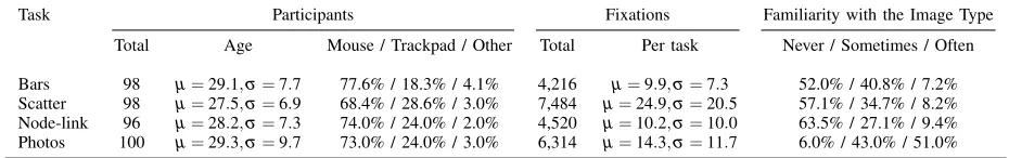
[image:7.567.309.500.57.261.2]

(8)

Task Participants Fixations Familiarity with the Image Type

Total Age Mouse / Trackpad / Other Total Per task Never / Sometimes / Often

Bars 98 µ=29.1,σ=7.7 77.6% / 18.3% / 4.1% 4,216 µ=9.9,σ=7.3 52.0% / 40.8% / 7.2%

Scatter 98 µ=27.5,σ=6.9 68.4% / 28.6% / 3.0% 7,484 µ=24.9,σ=20.5 57.1% / 34.7% / 8.2%

Node-link 96 µ=28.2,σ=7.3 74.0% / 24.0% / 2.0% 4,520 µ=10.2,σ=10.0 63.5% / 27.1% / 9.4%

[image:8.567.48.513.54.127.2]

Photos 100 µ=29.3,σ=9.7 73.0% / 24.0% / 3.0% 6,314 µ=14.3,σ=11.7 6.0% / 43.0% / 51.0%

TABLE 1: Summary of Turkers from Experiment 1. “Fixations” refers to the number of cursor presses that are used to focus on the stimulus. “Total” is the number of fixations for all participants on all five stimuli in each category. “Per task” shows the mean and standard deviation for the number of fixations per user, per stimulus.

compare these heatmaps to our ET gazes. The motivation for this step is to see how an off-the-shelf saliency detector compares to Fauxvea for predicting gaze during predefined analysis tasks. There are many saliency detectors available that take images as inputs and output smoothed saliency heatmaps; in this experiment, we demonstrate using Judd et al.’s model [23] that is trained using a benchmark set of eye-tracking data, and is therefore transparent for others to use. We report distances from ET to each of these gaze distributions in Sec. 4.6.

We computed distances from ET to each baseline.

• For Grid: a set of points were generated forming a

n×n grid on the stimulus, wheren is the square root

of the number of fixations in the gaze data.

• For Uniform, Centered, or Uniform+Centered: a set

of points was sampled from the distribution, using as many fixations as in the gaze data.

The distance between these baseline point data and the gaze data was computed using the algorithm described in Sec. 4.4 For the baselines involving a sampling procedure (all but Grid), distances were computed for 100 sampling iterations for each stimulus, then averaged.

For the Saliency baseline, we computed the average distance between ET and the model-generated saliency map for all stimuli. To compute each single distance score for a stimulus, we used the algorithm in Sec. 4.4 to get a normalized histogram of the ET gazes, then we normalized the model-generated saliency map as a histogram before applying the distance function.

4.6 Results

In this section, we report findings from our comparison of eye tracking and Fauxvea estimates for basic infovis charts and tasks (Sec. 4.6).

Summary statistics for our data collection experiments are shown in Table 1. Turkers performed 392 HITs from four different stimuli-task types. Eight Turkers submitted HITs without performing any Fauxvea cursor presses; therefore, their data are not included in our analysis.

In general, we found that fixations are distributed at sim-ilar locations between the eye-tracking (ET) and Fauxvea (MT) studies for all infovis stimuli. Heatmaps of fixation locations collected in Experiment 1 are shown in Figure 2, along with saliency map generated from the Judd model. Each row shows a sample visualization from our experi-ment, along with overlays of gaze data collected in ET and

MT studies. Red overlays show normalized maps of fixation locations both by eye-tracking participants and Turkers. All stimuli and heatmaps from Experiment 1 are available online at: [URL blinded - see Supplemental Materials PDF]. The similarities in these heatmaps between conditions

supportH1a. In most cases, white spaces in a visualization

are not fixated on in either eye tracking or Fauxvea, and the most relevant marks for the analysis task are fixated

on most heavily. Evidence supporting H1b is clearest in

the heatmaps of bar chart and scatter plot, where specific axis labels corresponding to correct task responses (i.e., column heights or (x, y) coordinate values) are fixated on heavily while the others are largely ignored. Heatmaps can also illustrate what visual-analysis strategies are used to complete tasks with less structure that do not use guide marks. For example, it is clear that people primarily fixate on faces in both eye-tracking and Fauxvea results to answer

the photograph task“Estimate the average age of all people

in the photo”and not other context clues (see Figure 2 for

an example).

We found quantitative evidence that fixation estimates made with Fauxvea are more similar to eye tracking than the baseline estimates we tested. While it is not surprising that Fauxvea performs better than random and task-agnostic gaze estimates, the results confirm a basic requirement for the method and also demonstrate how to quantitatively compare two sets of fixation locations. As we discuss in Sec. 7, opportunities exist to use this evaluation approach to compare new models of gaze against each another.

The distance between ET and MT (0.39 using the sym-metric KL function, 0.23 using the chi-squared function) is significantly less than the distance between ET and each

of the baselines (p< .001 for all paired, two-tail t-tests),

which supportsH2. Figure 3 shows the average distance for

both symmetric KL divergence andχ2_{distance between all}

ET and MT data, and the difference between ET data and each of the baselines we considered.

(9)

Image type Symmetric KL Divergence χ2_Distance

Uniform+Gaussian Gaussian Uniform Grid Uniform+Gaussian Gaussian Uniform Grid

Eye tracking

Scatter 1.09 8.10 0.75 0.73 0.83 1.35 0.65 0.64

Bars 1.60 9.84 1.08 1.07 1.11 1.63 0.84 0.84

Node-link 1.20 2.25 1.52 1.51 0.90 0.96 1.13 1.13

[image:9.567.290.526.208.384.2]

Photos 0.98 3.90 0.96 1.07 0.75 0.98 0.87 0.86

TABLE 2: Distance from eye-tracking data on different visualization types to random gazes from four baseline distributions. For each distance function, bold values show the distribution that most closely fits the image type (smallest distance score). These values suggest which null distribution is the fairest to sample for baseline comparisons against Fauxvea gaze estimates, for each of the four stimuli-task types we evaluated.

near the image center.

Finally, we performed a preliminary analysis of

se-quences of fixations, orscan paths, to compare the temporal

aspect of gazes between ET and MT data. Fixation locations from each participant were ordered by time, then dynamic time warping (DTW) was used to compute a table of similarity scores between all scan paths. The result is a set of high-dimensional points that represent each scan path. We used multidimensional scaling (MDS) to plot these scan paths as points in 2D and looked for areas where MT and ET points representing the same visualization tasks clustered together.

While a full analysis comparing sets of scan paths is beyond the scope of this paper, we found some evidence that MT scan paths for the same task cluster together when transformed by DTW. However, this clustering approach was not conclusive for comparing ET and MT scan paths. In the MDS plots, the ET scan paths appear more scattered than MT, and the small number of ET data points for each visualization task (from 18 eye-tracking participants) compared to the MT data makes it difficult to spot patterns in these plots between sets of scan paths. More work is needed to effectively compare different-sized sets of scan paths, like datasets from a controlled eye-tracking study and a larger crowdsourced study using Fauxvea.

5 E

XPERIMENT

2

We performed a small-scale follow-up experiment to test whether people with experience and interest in eye tracking are able to reliably predict fixation locations for the tasks and stimuli in Experiment 1. We wanted to know whether it is viable for a person to self-assess where gazes happen dur-ing a visualization task instead of runndur-ing a crowdsourced study with Fauxvea or performing an eye-tracking study.

5.1 Methods

We recruited six participants (four male, two female) who were researchers in human-computer interaction or com-puter vision at a major research university in the U.S. Each was right-handed, had normal or corrected-to-normal vision, and identified himself as having experience or in-terest in learning where people look in images. The ages of participants ranged from 25–35 years (M=28.7, SD=4.13). All participants passed an Ishihara test for normal color vision.

Fig. 5: Human predictions of fixation locations for the task “Estimate the value (height) at year 2007”. Six participants with experience in eye tracking and/or vision (P1–P6, identified in the figure with unique colors) marked five or more predicted locations for where other people will fixate.

In the first task, each participant was seated about 18 inches from a 24” 1920 x 1200 pixel monitor and viewed each of the 20 task-stimulus pairs from Experiment 1. For

each task, participants were asked to select at least five

locations in the stimulus they believe people performing the task will fixate on. Participants indicated their fixation loca-tions by clicking a cursor at localoca-tions inside the image. The tasks were presented in the same order that participants in the eye-tracking condition (ET) in Experiment 1 performed them. We recorded each predicted fixation location.

(10)

5.2 Results

The results from this study are primarily qualitative for two reasons: 1) recruiting a large sample size of people with experience in vision or eye tracking is difficult; 2) when asked to select fixation locations, most participants selected only the minimum number of locations we requested. Therefore, the data are sparse.

We examined the results from the first task by visualizing all fixations predicted by the expert participants and looking for patterns in how participants chose points across stim-uli. We created a filterable visualization of these fixation predictions that is available online at [URL BLINDED – screenshots in Supplemental Materials PDFs]. In general, we found that most participants identified similar key areas in each stimulus, but predictions varied in how people attend to areas of the stimuli that are visual salient but irrelevant to the particular tasks. Figure 5 shows an example where 5 of 6 participants predicted that others would fixate on the top of the column, x-axis guide marks, and y-axis guide marks corresponding to the task; however, there was little consensus on which other bars or guide marks people would attend. One participant (P2), a graduate student who studies eye tracking, did not predict any fixations on the task-specific areas of the bar chart; in a follow-up interview, she indicated that she focused on marking only visually salient regions.

Our main insight is that even with expertise in thinking about where others will gaze in an image, as an individual it is difficult to predict how a population of people will gaze during a visual analysis task. Several participants commented that they made predictions by first solving the task on their own, then reporting where they gazed during that trial; however, this strategy limits the evaluator to only one perspective and is not viable for estimating gazes from a population that might analyze a visualization in different ways.

In the second task, the experts correctly identified the real eye-tracking heatmap with 68.3% accuracy on average. They incorrectly identified the Fauxvea heatmaps as eye tracking 23.3% of the time, and 8.3% of the time they selected “Too close to call”. In a follow-up interview, most participants indicated that when heatmaps were noisier it was an indicator of real eye tracking. P5, who had run eye-tracking studies prior to our experiment, commented that adding random noise to the Fauxvea heatmaps could make them look closer to the eye-tracking heatmaps.

6 E

XPERIMENT

3

We ran a third experiment to see if the Fauxvea method is able to reproduce findings about visual exploration behaviors from an existing eye-tracking study using tree visualizations. This follow-up was aimed at evaluating the external validity of Fauxvea beyond the basic visualization interpretation tasks in Experiment 1. We reproduced the task and three stimuli from an eye-tracking study of tra-ditional, orthogonal, and radial tree layouts [3]. Burch et al. note that these layouts are “frequently used in many

application domains, they are easy to implement, and they follow aesthetic criteria for tree drawing”.

In general, we hypothesize that fixation locations and transition frequencies reported in the original study will be reproduced by running a similar experiment with Fauxvea (H3). In addition, we hypothesize that the three findings in the section titled “Analysis of Exploration Behavior” in [3] will be corroborated with data collected from a reproduction of the experiment using Fauxvea instead of an eye tracker (H4a, H4b, H4c).

H3 Transition frequencies between predefined areas of

interest (AOIs) in the original study will be similar to transition frequencies reproduced using Fauxvea.

H4a Participants will jump more frequently between leaf

nodes that are near each other in the traditional layout compared to the orthogonal and radial layouts.

H4b The pixel distance between the marked leaf nodes will

affect the transition frequency.

H4c Participants viewing the radial layout will transition

back from the root node to AOI 2 more frequently compared to the traditional and orthogonal layouts.

We evaluateH3in Sec. 6.3 by analyzing the most frequent

destination AOI from each source AOI. We evaluateH4a,

H4b, andH4cin Sec. 6.3 by analyzing specific patterns in

the corresponding transition tables.

Testing these hypotheses will help us evaluate whether Fauxvea can reproduce findings about visual exploration visualization without using an eye tracker. We note that we do not compute distance scores, as we did in Experiment 1, because the fixation data from the eye-tracking study are not available. Furthermore, rather than measuring how closely the Fauxvea estimates match the eye-tracking heatmaps, the main goal of this experiment is to corroborate or reject the findings from [3] using a similar analysis.

6.1 Stimuli and Tasks

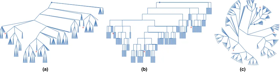
Participants were shown tree diagrams with marks that indicated the root node and three target nodes. Stimuli were composed of three tree layouts: traditional, orthogonal, and radial. The layouts differ in how nodes and edges are aligned. These layouts are shown in Figure 6. The

participants were asked to find theleast common ancestor

(LCA) of the target nodes in each tree. The instructions included a definition of the LCA written in plain English.

We asked participants to report the coordinates of the LCA for each tree they analyzed, so we added an in-teraction to the Fauxvea interface that lets users find the coordinates over the cursor location. While interacting with the interface, the user can type the ‘Return/Enter’ key to place a mark under the cursor and its (x, y) coordinates are displayed on the screen. In this way, participants can quickly find the coordinates of locations in the image without interfering with cursor presses.

6.2 MTurk Study

(11)

[image:11.567.40.504.56.177.2]

(a) (b) (c)

Fig. 6: Three stimuli for Experiment 3: (a) traditional, (b) orthogonal, and (c) radial tree layouts. The root node is indicated by a larger circle mark, and the target nodes for the common-ancestor task are indicated by red arrows.

each. We restricted each participant to one HIT only because the same underlying graph data is visualized in each HIT. All participants were located within the United States.

In each HIT, participants performed three training tasks using Fauxvea and were shown example trees with the LCA labelled to help them understand the task. For the fourth task, participants completed the task for the test stimulus that was replicated from the Burch et al. study. The test stimulus did not have the LCA labelled. During each HIT, participants could advance to the next image in the sequence after any amount of time by providing and answer to the question and clicking a button on the webpage. They were not allowed to revisit past images after moving on. We expected that each HIT would take 4-5 minutes to complete and paid each Turker who completed a HIT $0.45. A $0.15 bonus was offered to each Turker who identified the LCA correctly according to an expert reviewer.

After the visual analysis tasks, we collected demographic information about participants’ age, sex, and cursor device (mouse, trackpad, or other), as well as how often they look at images like these (“never”, “sometimes”, “often”) and general feedback about the strategy each Turker completed the LCA task.

6.3 Results

For each HIT, 85 Turkers performed the LCA task using the Fauxvea interface. Each of the test tasks was deemed accurate if the reported coordinates for the LCA were within 10 pixels of the known answer. Turkers who were accurate were given a $0.15 bonus. The average task accuracy for the HITs differed: Turkers were most accurate with the orthogonal layout (50.6% = 43/85), slightly less accurate with the traditional layout (41.2% = 35/85), and least accurate with the radial layout (20% = 17/85).

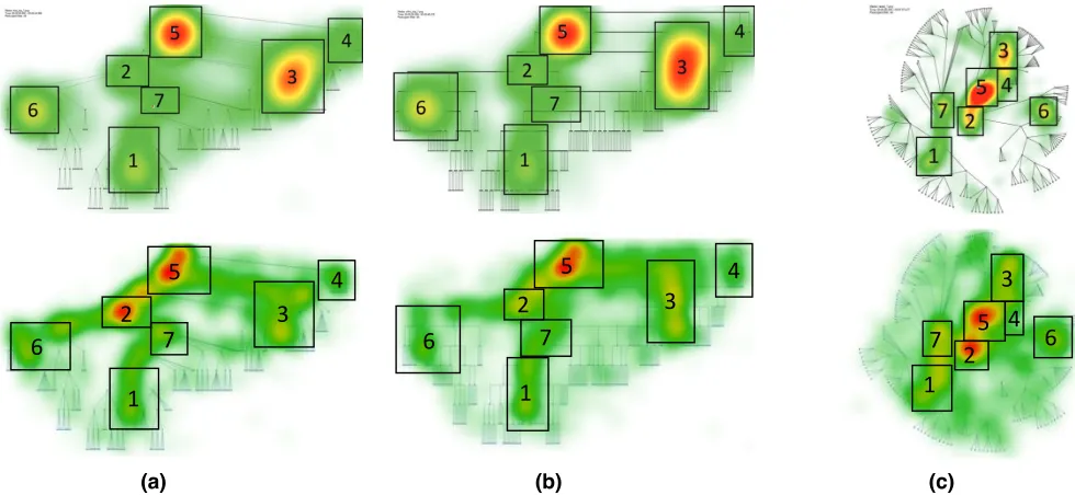
Overall, we found that the distributions of fixations from Experiment 3 on the three stimuli were similar to those published in Burch et al. [3]. In Figure 7, we show heatmaps of fixations from Experiment 3 alongside those from the original study. The top row shows fixation heatmaps and the AOIs specified in the original study. The second row shows heatmaps we generated from the data collected in Experiment 3. We implemented a heatmap

renderer using a rainbow color map to approximate the visualization technique in the earlier work; therefore, some visual differences between these charts may be due to implementation differences.

We observed several similarities between the heatmaps from the original study and Experiment 3. In all heatmaps, AOI 5 – which contains the root node of the tree – is fixated on heavily. This makes sense because locating the root node is critical for the task of finding the LCA of the target nodes. We also found subtrees and leaf nodes that were essentially ignored in both the original study and in Experiment 3. These include areas that are dense with nodes and edges but are not parts of the visualization that one must attend to find the LCA (e.g., between AOI 1 and AOI 3 in the traditional and orthogonal layouts). This suggests Turkers are able to focus on the task at hand and do not spend effort fixating on areas of the visualization that are irrelevant to the task, even if those areas are comparably visually salient in the blurred viewer. The fact that the heatmaps are similar between studies, and that they show evidence participants

fixate on task-specific areas, supports bothH1aandH1b.

We did not evaluateH2for Experiment 3 because the raw

eye-tracking data needed to compute quantitative distance scores were not available.

We also observed some differences between the fixation maps from these experiments. In general, the original eye-tracking fixations appear more focused and less spread out than the Fauxvea fixations. This contrasts our earlier findings in Experiment 1. An exception to this is the set of Fauxvea fixations that occur along edges in the traditional and orthogonal layouts (e.g., between AOI 2 and AOI 6, and between AOI 1 and AOI 7). Another noticeable area where heatmaps differ in the traditional layout is AOI 2, which is fixated on relatively more than AOI 3 in our experiment and less than AOI 3 in the original experiment. In this layout, Turkers were much more likely to transition from AOI 7 to AOI 2 than to any other AOI; in the original eye-tracking study, AOI 2 was also the most frequent transition from AOI 7, but AOI 1 and AOI 3 are other common destinations

(each with>10% frequency).

(12)

[image:12.567.36.526.52.278.2]

(a) (b) (c)

Fig. 10. Top row: Hierarchy dataset with three marked leaf nodes (stimuli data). Second row: Gaze plots for the same hierarchy dataset as illustrated in the top row. Third row: Heat maps for area of interest (AOI) determination based on the gaze plot data represented in the second row. Bottom row: Probabilities for direct transition between AOIs. Matrix entries highlighted in the same color belong to the same AOI pair.

showed that differences between radial and other layouts were signifi-cant (p<0.005, Bonferroni-corrected for multiple comparisons).

Hypothesis 2 can be confirmed. Non-radial layouts are significantly faster than the radial layout when performing the task of finding the least common ancestor of a set of marked leaf nodes. To understand the reasons for the longer duration when solving the task we have to take into account the eye movement data. There is no significant dif-ference between traditional and orthogonal layouts.

5.3 Effect of Number of Leaf Nodes Marked

Finally, we analyzed the effect of the number of leaf nodes marked in a diagram. First, an ANOVA analogous to the one in Section 5.1 showed that there was a significant effect of the number of marked leaf nodes on completion time (F(2,70) =5.72;p<0.005;h2=0.69)

with mean times 12.73s(SD=6.96s) for three marks, 14.85s(SD=

8.24s) for six marks, and 16.01s (SD=9.82s) for nine marks (see

Figure 8). The ANOVA analogous to Section 5.2 supports these re-sults. Here, the number of marked leaf nodes also had a significant ef-fect (F(2,70) =5.72;p<0.005;h2=0.62) with mean times 13.83s

(SD =8.92s) for three marks, 15.75s (SD=10.29s) for six marks, and 17.86s (SD =11.89s) for nine marks (see Figure 9). Post-hoc

pairwise testing revealed significant differences only between three and nine marks (p<0.005, Bonferroni-corrected for multiple

com-parisons). Since both analyses agree on this and an increasing number of marked leaf nodes results in increasing completion times, we con-firm Hypothesis 3.

5.4 Analysis of Exploration Behavior

We base our analysis of the participants’ exploration behavior on areas of interests (AOIs) that we derived from the density of the heat map representations. The top row of Figure 10 shows the same hierarchy dataset in the traditional, orthogonal, and radial layouts. The second row of Figure 10 represents gaze plots of the participants by the inte-grated visualization of the eye tracking system for the stimuli based on the datasets from Figure 10 (top row). Each participant is mapped to a different color as given by the integrated eye tracking software and all gaze trajectories are drawn on top of each other. An immense amount of visual clutter is produced and only the hot spots can be de-rived from this visualization. Therefore, we preprocess the data by first generating heat map representations as shown in Figure 10 (third row) to classify a set of regions that were of special interest for the subjects.

For the analysis, we calculated a transition matrix of the AOIs that contains the relative amount of direct transitions between each AOI to any other AOI, see Figure 10 (bottom). The transition matrix shows the probability to switch from one AOI to another without detours.

The goal of this analysis is to identify major differences in the ex-ploration behavior between the three layout strategies. This analysis method ignores the substantial amount of transitions that begin and end up outside of AOIs (denoted in the first row/column of the tran-sition matrix in Figure 10 (bottom)). To identify detailed characteris-tics of exploration strategies and to obtain statistically significant and quantitative findings, a more complete analysis approach should be followed, which is left for future work. However, for the comparative and qualitative investigation of the main differences in exploration

be-(a) (b) (c)

Finally, we analyzed the effect of the number of leaf nodes marked in a diagram. First, an ANOVA analogous to the one in Section 5.1 showed that there was a significant effect of the number of marked leaf nodes on completion time (F(2,70) =5.72;p<0.005;h2₌₀_.₆₉₎

8.24s) for six marks, and 16.01s(SD=9.82s) for nine marks (see Figure 8). The ANOVA analogous to Section 5.2 supports these re-sults. Here, the number of marked leaf nodes also had a significant ef-fect (F(2,70) =5.72;p<0.005;h2₌₀_._{62) with mean times 13}_._83s

(SD=8.92s) for three marks, 15.75s(SD=10.29s) for six marks, and 17.86s(SD=11.89s) for nine marks (see Figure 9). Post-hoc

be-(a) (b) (c)

Finally, we analyzed the effect of the number of leaf nodes marked in a diagram. First, an ANOVA analogous to the one in Section 5.1 showed that there was a significant effect of the number of marked leaf nodes on completion time (F(2,70) =5.72;p<0.005;h2=0.69)

8.24s) for six marks, and 16.01s (SD=9.82s) for nine marks (see

Figure 8). The ANOVA analogous to Section 5.2 supports these re-sults. Here, the number of marked leaf nodes also had a significant ef-fect (F(2,70) =5.72;p<0.005;h2=0.62) with mean times 13.83s

(SD=8.92s) for three marks, 15.75s (SD=10.29s) for six marks, and 17.86s (SD=11.89s) for nine marks (see Figure 9). Post-hoc

be-5

5

2

6

1

6

3

4

7

(a) (b) (c)

Fig. 7: Comparison of results from Experiment 3 with the results reported by Burch et al. Data in columns (a), (b), and (c) correspond to traditional, orthogonal, and radial layout conditions. Rows 1 and 2 show the eye-tracking heatmaps from Burch et al. and the gaze estimate heatmaps we collected in Experiment 3, respectively.

tradi&onal* source'

outside' AOI'1' AOI'2' AOI'3' AOI'4' AOI'5' AOI'6' AOI'7'

de

s5

na5

on'

outside' :% 68%% 40%% 59%% 27%% 50%% 49%% 39%% AOI'1' 11%% :% 5%% 2%% 3%% 2%% 6%% 4%% AOI'2' 20%% 7%% :% 2%% 1%% 11%% 23%% 41%% AOI'3' 18%% 3%% 7%% :% 29%% 18%% 6%% 5%% AOI'4' 4%% 0%% 0%% 3%% :% 9%% 0%% 0%% AOI'5' 25%% 3%% 20%% 27%% 31%% :% 11%% 4%% AOI'6' 10%% 7%% 13%% 2%% 5%% 6%% :% 4%% AOI'7' 8%% 9%% 12%% 2%% 0%% 0%% 3%% :%

Gomez%et%al.%

radial* source'

de

s5

na5

on'

outside' :% 61%% 42%% 28%% 11%% 26%% 64%% 42%%

AOI'1' 24%% :% 8%% 2%% 0%% 2%% 3%% 18%%

AOI'2' 20%% 9%% :% 5%% 2%% 29%% 17%% 26%%

AOI'3' 12%% 4%% 3%% :% 23%% 23%% 1%% 2%%

AOI'4' 1%% 0%% 1%% 9%% :% 7%% 5%% 0%%

AOI'5' 16%% 2%% 20%% 46%% 51%% :% 7%% 8%%

AOI'6' 14%% 2%% 5%% 5%% 11%% 4%% :% 0%%

AOI'7' 11%% 20%% 17%% 1%% 0%% 6%% 1%% :%

Gomez%et%al.%

orthogonal* source'

de

s5

na5

on'

outside' :% 49%% 57%% 65%% 56%% 58%% 68%% 47%%

AOI'1' 10%% :% 2%% 3%% 0%% 3%% 3%% 26%%

AOI'2' 12%% 2%% :% 0%% 0%% 11%% 12%% 18%%

AOI'3' 23%% 4%% 3%% :% 23%% 14%% 4%% 2%%

AOI'4' 6%% 0%% 0%% 10%% :% 3%% 0%% 1%%

AOI'5' 29%% 2%% 27%% 19%% 20%% :% 8%% 3%%

AOI'6' 10%% 7%% 2%% 1%% 0%% 5%% :% 1%%

AOI'7' 6%% 32%% 7%% 0%% 0%% 1%% 2%% :% Gomez%et%al.%

orthogonal* source'

de

s5

na5

on'

outside' :% 55%% 38%% 41%% 45%% 42%% 66%% 43%%

AOI'1' 17%% :% 10%% 1%% 3%% 7%% 2%% 16%%

AOI'2' 12%% 5%% :% 2%% 0%% 5%% 10%% 25%%

AOI'3' 28%% 3%% 16%% :% 36%% 32%% 5%% 6%%

AOI'4' 4%% 0%% 2%% 11%% :% 7%% 0%% 0%%

AOI'5' 16%% 3%% 21%% 43%% 15%% :% 15%% 8%%

AOI'6' 17%% 7%% 5%% 1%% 0%% 4%% :% 2%%

AOI'7' 5%% 27%% 10%% 1%% 0%% 3%% 2%% :% Burch%et%al.%

radial* source'

de

s5

na5

on'

outside' :% 56%% 17%% 12%% 8%% 16%% 33%% 40%% AOI'1' 21%% :% 10%% 1%% 1%% 4%% 4%% 15%% AOI'2' 16%% 14%% :% 4%% 3%% 22%% 36%% 28%% AOI'3' 15%% 1%% 5%% :% 23%% 31%% 4%% 0%% AOI'4' 1%% 0%% 2%% 43%% :% 16%% 7%% 2%% AOI'5' 17%% 8%% 42%% 35%% 62%% :% 15%% 15%% AOI'6' 14%% 1%% 13%% 4%% 4%% 9%% :% 0%% AOI'7' 16%% 20%% 10%% 0%% 0%% 2%% 0%% :%

Burch%et%al.%

tradi&onal* source'

de

s5

na5

on'

outside' :% 59%% 35%% 59%% 22%% 35%% 36%% 47%%

AOI'1' 17%% :% 11%% 3%% 4%% 8%% 17%% 13%%

AOI'2' 6%% 3%% :% 0%% 0%% 4%% 31%% 18%%

AOI'3' 26%% 5%% 11%% :% 40%% 24%% 0%% 11%%

AOI'4' 6%% 1%% 0%% 10%% :% 17%% 3%% 0%%

AOI'5' 25%% 3%% 15%% 26%% 33%% :% 12%% 5%%

AOI'6' 12%% 19%% 9%% 0%% 0%% 11%% :% 5%%

AOI'7' 7%% 10%% 20%% 1%% 0%% 1%% 2%% :% Burch%et%al.%

(a) (b) (c)

Fig. 8: Comparison of results from Experiment 3 with the results reported by Burch et al. Data in columns (a), (b), and (c) correspond to traditional, orthogonal, and radial layout conditions. Rows 1 and 2 show transition probabilities between AOIs from Burch et al. and the probabilities we found in Experiment 3, respectively. Transition probabilities to or from areas outside any AOI are grayed out. Green cells indicate where the most likely destination AOI from a source is the same in both the eye-tracking results and the Experiment 3 results. Yellow cells indicate where the most likely destination AOI from a source was not the same in both eye-tracking and Experiment 3 results.

eye-tracking study, and the second row shows probabilities from the data in our experiment. The similarity in transi-tion tables between experiments suggest that participants explored the AOIs using similar patterns. For 14 out of the 21 source AOIs in the three layouts (67%), the most frequent destination AOI (highlighted in green) was the same in both the original results and our results. This is

much better than the 3 or 4 matches (16.7% =1/6) we

expect if the most frequent destination from each AOI were randomly chosen from the remaining six. Therefore, we

find support for H3. The cells highlighted in yellow show

where the most likely destination AOI is different between the experiments. In all but one of these cases, the most likely transition in our experiment was the second most likely in the original experiment.

Examining the transition probabilities, we did not find

support for H4a. Burch et al. found that the probability

[image:12.567.37.528.332.516.2]

(13)

We found partial support forH4b. We re-examined the

transitions that supported this hypothesis in the original study. The Fauxvea transition probability from AOI 1 to AOI 3 (and vice versa) is less than the probability from AOI 1 to AOI 6 (and vice versa) in the traditional (3% (2%) compared to 7% (6%)) and orthogonal (4% (3%) compared to 7% (3%)) layouts. The distance between AOIs 1 and 3 is greater than the distance between AOIs 1 and 6. However, for the radial layout, we found that the probability from AOI 1 to AOI 3 (and vice versa) was not necessarily less than the probability from AOI 1 to AOI 6 (and vice versa), as in the eye-tracking study: 4% (2%) compared to 2% (3%). In fact, the distances from AOI 1 to AOI 3 and AOI 6 are not as different in the radial layout and in the traditional and orthogonal ones (see Figure 6). We discuss possible explanations for these differences in Sec. 7.1.

Finally, we found strong support forH4c. In our

experi-ment, the probability from AOI 5 to AOI 2 is 29% in the ra-dial layout but only 11% in both traditional and orthogonal layouts. This is comparable to Burch et al.’s probabilities for this transition: 22% (radial), 4% (traditional), and 5% (orthogonal).

7 D

ISCUSSION

In this section, we discuss how Fauxvea might affect visual exploration behaviors, then we outline opportunities for improving Fauxvea and quantitative comparison methods for gaze estimates.

7.1 Visual Exploration Behaviors

We noticed a few differences in how eye-tracking and Fauxvea fixations are distributed spatially for visualization tasks. In Experiment 1, we found that eye-tracking gazes generally occur over wider regions of the image and appear more spread out than Fauxvea gaze estimates (see Figure 2). There are several possible explanations for this behavior:

• People do not look at a singular point of interest for

long; instead, their gaze hovers around that point.

• Holding a cursor at a single pixel location over time

requires less effort than gazing at one location for the same amount of time.

• The time and effort needed to move and press the

cursor is greater than a saccade of the eye.

• For Turkers, there is an opportunity cost to being slow

or getting distracted by irrelevant image details. We expected that Turkers would finish the HITs for this experiment as quickly as possible in order to accept new HITs and to maximize their payments on MTurk.

• Eye trackers can have errors due to both calibration

and moments when the eye tracker cannot find the eye. Therefore, recorded coordinates might be inexact. Our findings in Experiment 3, which involves a more complex task, show a different pattern: in some cases, Fauxvea gaze estimates are more spread out than eye-tracking gazes (see the radial layout in Figure 7). It is possible that Turkers using the Fauxvea interface had less

experience with this task compared to the participants in the eye-tracking study and therefore spend more time exploring the diagram. Turkers also used the interface to fixate on edges in the tree diagrams more than eye-tracking participants, which supports the idea that they focus on tracing paths to complete the task. Eye-tracking participants with the normal viewer, on the other hand, can make saccades between nodes and may rely on peripheral vision to view edges. In both populations, similar hot spots related to the task appear in the heatmaps.

7.2 Quantitative Comparisons

In Experiment 1, we compared Fauxvea fixations against eye-tracking fixations using a quantitative approach similar to an earlier evaluation by Rudoy et al. [15]. We evaluated an additional distance function and tested additional base-line distributions of random fixations, plus a grid basebase-line and a saliency model. We discuss our findings below.

7.2.1 Distance Metrics

We explored two measures of similarity between smoothed representations of gaze locations: a symmetric version of

KL divergence andχ2_{distance. Figure 4 shows one of these}

metrics (χ2_{) computed between the ET and MT data we}

collected, for each pair of stimuli-tasks. As a sanity check, we were interested in seeing how values on the diagonal – which are distances between corresponding visualization tasks in the two conditions – compare to distances between unrelated visualization tasks. We note that this type of matrix should not necessarily be symmetric across the diag-onal, because the columns (Fauxvea) represent a different modality for which fixations were collected compared to the rows (eye tracking). The matrix shows that the diagonal is in fact darker than any single row. This is also visual

evidence of hypothesis H1b: the fixations from both ET

and MT are linked to underlying visualization tasks.

7.2.2 Generating Baseline Gazes

We evaluated Fauxvea quantitatively by computing how much closer to eye tracking Fauxvea’s fixation locations are compared to fixations drawn from simple null distributions; creating more realistic computational models of gaze during visualization analysis is an open problem that is beyond the scope of this paper.

We used an off-the-shelf, state-of-the-art model of visual saliency [23] and found that the maps it generates from the visualization stimuli in Experiment 1 are not much closer to eye tracking than the other null distributions, like Grid and Centered Gaussian. This is not surprising because people do not necessarily attend to salient regions that are irrelevant to the analysis task they are given. It is possible that people with experience in vision and eye tracking could identify where people will look during tasks, but as we found in Experiment 2, self-assessment of these areas is not consistent even among experts.