Partitioned block frequency domain prediction error method based acoustic feedback cancellation for long feedback path

Partitioned Block Frequency Domain Prediction

Error Method based Acoustic Feedback Cancellation

for long feedback path

Alessio Izzo

, Ludovico Ausiello

, Carmine Clemente

and John J. Soraghan

† _{HouseYellow Acoustic and Audio Consulting. E-mail:ludwig.ausiello@gmail.com}

Abstract—In this paper an innovative method of using Acous-tic Feedback Cancellation (PEM based PBFD-AFC) in large acoustic spaces is presented. The system under analysis could vary from Single Source Single Receiver (SISR) to a Multiple Sources Multiple Receivers (MSMR). An environment is representative of (e.g.) churches installations or Public Address (PA) systems, thus involving the presence of one or more microphones and corresponding feedback paths. The Partitioned Block approach consists of slicing the feedback path (e.g the impulse response of the system) to improve the algorithm performance. It can be applied either in the time domain or in the frequency domain, where the latter, called Partitioned Block Frequency Domain, shows faster convergence, lower computational cost and higher estimation accuracy. The results of the proposed framework is compared with the state of the art using real acoustic data showing superior performance with up to20dBMaximum Stable Gain (MSG) and30seconds less convergence time.

I. INTRODUCTION

Acoustic feedback is a relevant audio topic ever since the introduction of the first sound reinforcement and public address (PA) systems [1][2]. Also referred to as the Larsen Effect, the microphone, amplifier and loudspeaker are arranged in a closed loop, i.e. whenever a microphone captures information created in the environment, and then sends it to be played-back by a speaker placed in close proximity. Typically, as soon as the loop gain rises above a threshold, several undesired signals (howling, ringing, self-oscillations etc.) start affecting the system performance and degrades both sound intelligibility and sound quality.

In the past 50 years several solutions have been proposed, modelled and implemented using both software and hardware [3]. For example a common method comprises placing notch filters into the signal path [3], [4]. Although correctly decreas-ing in the loop gain at those critical frequencies at which the problem arises, this approach has a main drawback: in that system can only react after howling or self-oscillations have occurred and cannot prevent the audience from experiencing these. On the contrary, there is a proactive approach, which is called Adaptive Feedback Cancellation (AFC). It is aimed at predicting the feedback signal component and then subtracting this prediction from the microphone signal [4]. In [5], [6], [7], [8] different proactive approaches wee presented for hearing aid applications. In the context of hearing aids the feedback path impulse response is less than5ms.

In this paper we focus a large acoustic rooms (with a rever-beration time R60 as long as 1-5 seconds [9]) and hence an alternative approach will be needed if an unbiased solution and

a fast convergence rate is required.

The aim of this paper is to show a new technique for an unbiased estimation of long acoustic feedback paths, im-proving the sound intelligibility in scenarios such as public address systems. After introduced the problem statement in the Section II, the standard technique for the IR estimation will be discussed in the Section III, addressing this using both the source signal model and regularization method. Then the proposed new algorithm will be introduced in Section IV. Finally, section V will present and discuss the performance in terms of Misalignment (MSL) and Maximum Stable Gain (MSG) using real acoustic data, demonstrating the goodness of the Partiotioned Block Frequency Domain (PBFD) approach.

II. PROBLEM STATEMENT

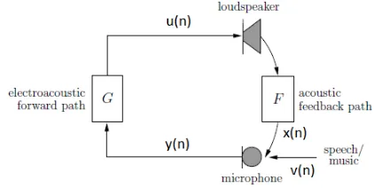
Consider for simplicity the loudspeaker single-microphone (SISO) system depicted in Figure 1.

Figure 1: Acoustic Feedback in a single input single output (SISO) scenario.

Let y(n)be the microphone signal defined as:

y(n) =x(n) +v(n), (1) where the feedback signal x(n) = f(n)∗u(n) is the con-volution of the finite impulse response (FIR) filter f(n)(the acoustic feedback path) of lengthnF with the loudspeaker

sig-nalu(n)and thev(n)is the source signal, withnthe discrete time index. ConsideringF(q, n)the polynomial version of the time variant discrete time filter equal to:

F(q, n) =f0(n)+. . .+fnF−1(n)q

−(nF−1)_=fT_{(n)q, (2)} the feedback signal can be expressed also as:

with q =

1, q−1, . . . , q−(nF−1)T _{the delay operator, and} f(n) the FIR filter coefficients vector at the instant n. In a closed loop system, the far-end and near-end signals,u(n)and

v(n)respectively, are related by closed loop transfer function [10]:

u(n) = G(q, n)

1−G(q, n)F(q, n)v(n). (4)

According to the Nyquist’s criterion, the closed loop system becomes unstable if there exists a radial frequencyωfor which:

(

|G eiω, n

F ejω, n

| ≥1

∠G eiω, nF ejω, n= 2kπ, k∈Z

, (5) withF ejω, nandG eiω, nthe Short Time Fourier Trans-form (STFT) of the acoustic feedback path and electroacoustic forward path respectively, with the latter one equal to:

G(q, n) =g1(n)q−1+. . .+gnG(n)q

−nG_{. (6)} In (6) G(q, n) is assumed to contain at least one unit delay (g0(n)≡0). When the AFC method is applied, the scheme

depicted in figure 2 can be considered [4].

Figure 2: Acoustic Feedback Cancellation (AFC) basic scheme.

A FIR filterFˆ(q, n)is placed in parallel with the acoustic feedback path; its input is the loudspeaker signal u(n), and its desired output is the feedback signal. Accordingly, the feedback signal x(n) can be predicted by the adaptive filter output signal yˆ(n) = ˆF(q, n)u(n)which is subtracted from the microphone signal obtaining the error signal e(n)as:

e(n) =y(n)−Fˆ(q, n)u(n). (7) In this case the Nyquist’s criterion can be rewritten as follow:







|G eiω, nh

F ejω, n

−F eˆ jω, ni

| ≥1

∠G eiω, nh

F ejω, n

−F eˆ jω, ni

= 2kπ, k∈Z

,

(8)

withFˆ(q, n)being the estimated Room Impulse Response (RIR) of F(q, n). WhenFˆ(q, n)converges more to F(q, n), the feedback compensated signale(n)will get closer the near-end signalv(n), thus leading to better audio quality.

III. AFCFRAMEWORK

Most of linear adaptive filtering algorithms are related to the Least Squares (LS) estimate of the Room Impulse Response (RIR), given by [3]:

ˆ

fLS(n) = UTU

−1

UTy. (9)

A common problem in room acoustic application is that the matrix UTU is ill-conditioned. A standard technique to turn an ill-posed problem into a well-posed problem is to apply the regularization. In [4] and [7] the problem has been addressed with a weighted LS criterion, given by:

min ˆ

f

_h

y−Uˆfi T

Why−Uˆfi+

h

ˆ_f−ξiT_Φhˆ_f−ξi_.

(10)

with ξ a reference value, W and Φ the weighting matrices. The property of criterion in equation (10) will depend on the choice of the weighting matricesWandΦ. A straightforward choice is to minimize the Mean Square Error (MSE) criterion

min ˆ

f(n)

h

ˆ_f(n)−f(n)iTh

ˆ

f(n)−f(n)i

, (11) between the estimated and true RIR. The MSE optimal choice for the weighting matrices and for the reference value is

ξ =f0, W =Rv−1 and Φ = Rf−1, leading the optimally weighted and regularized LS estimate:

ˆ

f(n) =f0+ UTRv−1U+Rf−1

−1

UTRv−1(y−Uf0), (12) with f0 a reference value, Rv and Rf the autocorrelation matrices of the source signal and impulse response, respec-tively. Often the estimate of equation in (12) cannot be calculate because the autocorrelation matrices Rv and Rf are generally unknown. In [7], [11], [12], the source signal autocorrelation matrix Rv has been modelled with different Prediction Error Methods (PEM). In [13] both short-time prediction filter and long-time prediction filter are taken in account. In this paper only the short-time prediction filter is considered. Letv(n)be the source signal, it can be considered as v(n) = H(q, n)w(n) where w(n) is a white noise excitation signal and

H(q, n) = 1

A(q, n) =

1

1 +a1(n)q−1. . .+anA(n)q

−nA, (13) is the source signal autoregressive model (AR) that is a nA

order time varying linear filter. In this case, the autocorrelation matrix Rv can be factorized in the form [14]:

Rv−1=ATΣA, (14)

with Σ a diagonal matrix and A the AR coefficients matrix. Accordingly, the criterion in (10), with ξ =f0,W =Rv−1 and Φ=Rf−1, can be rewritten by shifting the pre-filtering matrix Ainto the data term hy−Uˆf(n)iobtaining:

min ˆ

f

h

˜ y−U˜ˆfi

T

Σ−1hy˜−U˜ˆfi+

h

ˆ

f−f0

iT

Rf−1

h

ˆ_f−f0i

,

(15)

with the pre-filtered loudspeaker and microphone signals de-fined as:

˜

U=AU, ˜y=Ay. (16)

The AR coefficients ai(n) have been efficiently computed

solution to an equation involving a Toepliz matrix, saving computational cost. If the final order is l, the algorithm runs in O(l2_{) time, despite Gauss-Jordan elimination which runs}

in O(l3_{) time. The source signal model A(q, n) has been}

estimated using a block-based scheme, where the block length roughly approximates stationary intervals of the source signal (approximately 20ms [5], [11]).

Taking in account also the true RIR covariance matrix

Rf = E

f(n)fT(n) , (17) the 3−parameter RIR model proposed in [16] has been con-sidered. In [17], the cited model is based on the observations of the RIR measured, which may be characterized by three parameters:

• initial delay d, which is the time it takes to the loud-speaker output to reach the microphone through the direct path;

• direct path attenuation A, which determines the peak response in the RIR;

• the exponential decay time constantτ, which models the envelope of the reverberant tail of the RIR.

These three parameters may be estimated from acoustical setup using Sabine’s reverberation formulas [16] and they can be considered as prior knowledge. If these three parameters are taken into account a diagonal estimate of the true RIR covariance matrix may be constructed as:

ˆ

Rf,3=A·diag







β . . . β

| {z }

d

,1, e−2τ,· · · , e−2nF −d τ







, (18)

withβ a small number (e.gβ= 10−6_{). The advantage of this}

model is thatτis related to the environment, so it’s invariant to the RIR changes due to microphone or loudspeaker movements and so do the parameters d and A, as long as the distance between loudspeaker and microphone remain constant. For this reason this RIR model is considered to be more robust to the RIR changes than the other RIR models. Finally, two particular choice of f0 are of special interest: f0=0 leads toTikhonov type of regularization (TR), whereas choosing f0= ˆf(n−1) yields a Levenberg-Marquardt type of regularization (LMR). By choosing the latter approach, the Normalized Least Mean Square (NLMS) algorithm can be straightforward derived from the criteria in (15), leading to the PEM based LMR-NLMS estimation of the RIR:

ˆ

f(n) = ˆf(n−1) +µ Rˆf,3u˜(n) ˜(n)

˜

uT_(n)Rˆ

f,3u˜(n) +σr2

, (19) with µ the step size of NLMS algorithm and ˜(n) = ˜y−

˜

Uˆf(n−1) the pre-filtered version of the error signal. IV. PROPOSEDMETHOD- PBTDANDPBFD

Despite the hearing aids environment, PA systems face much longer impulse responses. In particular it can be much longer than the maximum 20ms experienced in hearing aids. For example in a A×B meters space the RIR can last up to 5 seconds. Estimating a longer RIR means that higher computational costs needs to be accounted and a more efficient solution needs to be evaluated. In such scenarios, in order

to achieve both fast convergence and low misalignment, a Partitioned Block Time Domain (PBTD) of the PEM based LMR-NLMS algorithm could be used [18].

Letˆf(n)be the estimated RIR of ordernˆF =nF, thenˆF taps

feedback canceller ˆf(n) is partitioned into nˆF/P1 segments

ˆ

fp(n)of length P each: ˆ_{fp(n) =}h_fˆ

pP(n),fˆpP+1[n], . . . ,fˆ(p+1)P−1[n]

i

, (20) withp= 0, . . . ,nˆF

P −1. In this case, the equation in (19) will

become:

ˆ

fp(n) =ˆfp(n−1) +µp

Rfpu˜(n) ˜(n)

˜

uT_(n)R

fpu˜(n) +σ2r

, (21) where Rfp is the covariance matrix of the p-ith IR block.

Usually, while moving on to the IR tail, the loop gain |G(q, n)F(q, n)|will show a lower energy, thus producing a degraded estimation. To compensate this, a slower adaptation speed is preferable, leading to a choice of a Variable Step Size (VSS) µp, instead of a fixed one [6].

In order to get a faster convergence and a reduced complexity, a Partitioned Block Frequency Domain (PBFD) version of the algorithm has been designed [6], [18], [19]. The estimated IR in the frequency domain is obtained as:

ˆ Fp=F

_ˆ

fp(n) 0

withp= 0, . . . ,nˆF

P −1 (22)

whereFequals theM×M Discrete Fourier Transform matrix (DFT). Define the L-dimensional block signal umas

um= [u[mL+ 1], . . . , u[(m+ 1)L]] T

, (23) with m the block time index. For each block um of input

samples

˜

Up[m] =diag{F[Aum]}, (24)

the algorithm produces L output samples˜zm= [z[mL+ 1],

. . . , z[(m+ 1)L]]T:

˜zm= [0 IL]F−1

ˆ

nF/P−1

X

p=0

˜

Up[m]Fˆp[m], (25)

L is the block length. The corresponding input output delay of the PBFD implementation equals2L−1. To ensure proper operation, it is required that the DFT length M ≥P+L−1. The adaptive filter coefficients are updated using an ”overlap-and-save” method, producing (in the frequency domain) the error signal:

˜

E[m] =F

0 ˜ m

, (26) with ˜m = ˜ym − ˜zm and ˜ym = [˜y[mL+ 1], . . . ,

˜

y[(m+ 1)L]]T. Using the PEM based NLMS algorithm, the IR coefficients (in the frequency domain) are obtained as follow:

ˆ

Fp[m] =Fˆp[m−1] +∆[m−1]

h

FgF−1U˜H_p [m]E˜[m]i+

−∆[m−1]hηFˆp[m]−Fp,ref

i

,

(27)

1_Withnˆ

whereηis a diagonal matrix containing the trade off parameter

ηk, with k= 0, . . . ,nˆF/P,gis an adaptation matrix build as g=

IP 0

0 0M−P

, (28) Fp,ref represents the DFT of reference measure of the IR.

In frequency domain approach we express the regularization function as:

∆[m] =diag{µ0[m], . . . , µM−1[m]}, (29)

which is the diagonal matrix containing the VSSµk[m]:

µk[m] =

µk

|E˜k[m]|2+|U˜k[m]|2+δ

. (30) The normalization is used to reduce the excess error in pres-ence of signals with large power fluctuation. The denominator is the sum of the input power with the error power plus a small positive number δto avoid division by zero. Furthermore, the a-priori knowledge into the PBFD approach has been taken in account through Fp,ref, reducing the computational costs.

Involving both the PEM and the a-priori knowledge into the PBFD with VSS, the bias into the estimation of the IR of large acoustic space has been drastically reduced. In the Section V the performance of the enunciated algorithms will be compared.

V. SIMULATIONRESULTS

To assess the performance of the proposed algorithm, the Misalignment factor (MSL) and Maximum Stable Gain (MSG) have been considered. The former is used to track the discrepancy between the true and the estimated feedback path, and it is defined as:

M SL(n) =k

ˆ_f(n)−f(n)k

kf(n)k . (31) The latter is defined as the maximum allowable gain, assuming a flat frequency response of G(q, n)as follow:

M SG[dB] =

−20 log₁₀

max

ω∈P|J e

jω_{, n}h

F ejω, n

−F eˆ jω, ni

|

.

(32)

where P denotes the set of frequencies at which the phase condition in (5) is fulfilled. From (32) it immediately follow that a better estimation of the IR allows to get a larger MSG. The input signal of the simulations was a 10 seconds female voice speech sampled atfs= 16kHz; in all cases we

considered a PEM with filter order nA= 30. An

overlap-and-save method has been used to implement the PBFD; the IR block size has been set withP = 160, together with aM×M

DFT matrix with M = 2P. Since speech is considered to be stationary during20msframes, the block length of the source signal per each frame has been setted withV = 320 samples. The impulse responses have been measured into an anechoic chamber using sine sweep method [20] with a microphone placed 3 meters far away from the loudspeaker, varying both microphone and loudspeaker positions. The IRs length were approximately1.34slong each, equal tonF = 21447samples.

In the first simulation the basic NLMS algorithm performance has been compared with LMR-NLMS algorithm. Using the same step size value µ = 0.2 as control parameter of the

Figure 3: AFC performance with a female speech signal of10s

long with f s= 16kHz,nF = 21447, andnA = 30. a)

Mis-alignment factor (MSL): comparison among the NLMS and LMR-NLMS algorithms with fixedµ= 0.2, and PBTD, PFDF and PEM-PBFD algorithms with VVS µ= [0.2 0.08 0.02]; b) Maximum Stable Gain (MSG)comparison among the NLMS and LMR-NLMS algorithm.

Figure 4: AFC performance with a female speech signal of10s

long with f s= 16kHz,nF = 21447,nA = 30 and variable

step size VSS µ = [0.2 0.08 0.02] : PEM besed PBFD LMR NLMS with VSS in a non stationary feedback path scenario. a) Misalignment factor (MSL); b) Maximum Stable Gain (MSG).

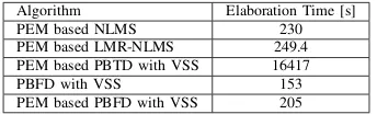
Table I: Elaboration time of the AFC algorithms with a female speech signal of 10s long with f s = 16kHz, nF = 21447,

nA= 30.

Algorithm Elaboration Time [s] PEM based NLMS 230 PEM based LMR-NLMS 249.4 PEM based PBTD with VSS 16417 PBFD with VSS 153 PEM based PBFD with VSS 205

slower convergence rate and a high computational cost. On the contrary, the frequency domain method avoids both problems. PBFD substantially decreases the computational burden, and shows a convergence rate faster than the all other algorithms, thus becoming a suitable choice for real time implementations.

VI. CONCLUSION

In this paper, a new framework to tackle the acoustic feedback problem in large acoustic spaces has been presented. It is based on the Frequency Domain Adaptive Filtering (FDAF) implementation of the Normalized Least Mean Square (NLMS) algorithm. Since the traditional LS-based adaptive filtering algorithm converge to a biased solution of the acoustic feedback path due to a considerable correlation between loud-speaker and microphone signals, a signal decorrelation method has been used. Inspired by hearing aids device, the Prediction Error Method (PEM) has been introduced. In order to further decrease the bias into the estimated feedback path, the

a-priori knowledge has been introduced through the Levenberg-Marquardt Regularization. The results show that this technique outperform previous approaches, achieving a lower estimation error and a faster convergence rate.

REFERENCES

[1] Tannoy LTD, “http://www.tannoy.com/prestige/Library.html,https://en. wikipedia.org/wiki/Tannoy,” 2016.

[2] C.R. Boner C. P. Boner, “Behavior of Sound System Response Immediately Below Feedback,” Journal of Audio Engineering Society, vol. 14, no. 3, pp. 200–203, July 1966.

[3] M. Moonen T. Van Waterschoot, “Fifty Years of Acoustic Feedback Control: State of the Art and Future Challanges ,” Proceedings of the IEEE, vol. 99, no. 2, pp. 288–327, February 2011.

[4] T. Van Waterschoot,Design and evaluation of Digital Signal Processing algorithms for acoustic feedback and echo cancellation, Katholieke Universiteit Leuven, 2009.

[5] M. Moonen J. Wouters A. Spriet, I. Proudler, “Adaptive Feedback Cancellation in Hearing Aids With Linear Prediction of the Desired Signal,” IEEE Transactions on Signal Processing, vol. 53, no. 3, pp. 3749–3763, October 2005.

[6] M. Moonen J. Wouters A. Spriet, G. Rombouts, “Adaptive feedback cancellation in hearing aids,”Elseiver, Journal of the Franklin Institute, vol. 343, no. 3, pp. 545–573, August 2006.

[7] M. Moonen T. Van Waterschoot., G. Rombouts, “Optimally regularized adaptive filtering algorithms for room acoustic signal enhancement,” Elsevier Signal Processing, vol. 88, no. 3, pp. 594–611, March 2008.

[8] J. Hellgren, “Analysis of feedback cancellation in hearing aids with Filtered-x LMS and the direct method of closed loop identification,” IEEE Transaction on Speech and Audio Processing, vol. 10, no. 2, February 2002.

[9] R. Spagnolo, Manuale di acustica applicata, UTET Libreria, 2002. [10] M. Moonen T. Van Waterschoot, “Adaptive Feedback Cancellation for

audio application,” Elseiver, Journal of the Franklin Institute, vol. 88, no. 11, pp. 2185–2201, November 2009.

[11] M. Moonen T. Van Waterschoot, G. Rombouts, “On the performance of decorrelation by prefiltering for adaptive feedback cancellation in public address system,”Proceedings of the 2004 IEEE Benelux Signal Processing Symposium, Hilvarenbeek, Netherlands, pp. 167–170, April 2004.

[12] P. Verhoeve M. Moonen T. Van Waterschoot, G. Rombouts, “Double-talk robust Prediction Error Identification Algorithms for Acoustic Echo Cancellation,”IEEE Transactions on Signal Processing, vol. 55, no. 3, pp. 846–858, March 2007.

[13] D. Freitas B. C. Bispo, “Performance Evaluation of Acoustic Feedback Cancellation Methods in Single-Microphone and Multiple-Loudspeakers Public Address Systems ,” International Conference on E-Business and Telecommunications, Springer, vol. 554, pp. 473–495, December 2015.

[14] L. Ljung, System identification: theory for the user, Prentice-Hall, Englewood Cliffs, NJ, 1987.

[15] S. Hykin, Adaptive Filter Theory, Prentice-Hall, Upper Saddle River, USA, NY, 2002.

[16] W.C. Sabine, Collected papars on acoustics, Peninsula, Los Altosl, California, 1992.

[17] M. Moonen T. Van Waterschoot, G. Rombouts, “Towards optimal regularization by incorporating a priopi knowledge in an acoustic echo canceller,” Proceedings of the 2005 IEEE International Workshop on Acoustic Echo and Noise Control (IWAENC 05), Eindhoven, Nether-lands, pp. 157–160, 2005.

[18] S. Nordholm S. Doclo H. Schepker, L.T.T. Tran, “Improving adaptive feedback cancellation in hearing aids using an affine combination of filters,” IEEE ICASIP 2016, vol. 88, no. 3, pp. 231–235, March 2016. [19] M. Moonen S. H. Jensen J. M. Gil-Cacho, T. Van Waterschoot, “Adaptive feedback cancellation in hearing aids,” IEEE Transaction on Audio, Speech and language processing, vol. 22, no. 12, pp. 2074– 2086, December 2014.