City, University of London Institutional Repository
Citation:
Spreeuw, J. (2014). Archimedean copulas derived from utility functions. Insurance: Mathematics and Economics, 59, pp. 235-242. doi:10.1016/j.insmatheco.2014.10.002
This is the accepted version of the paper.
This version of the publication may differ from the final published
version.
Permanent repository link:
http://openaccess.city.ac.uk/5030/Link to published version:
http://dx.doi.org/10.1016/j.insmatheco.2014.10.002Copyright and reuse: City Research Online aims to make research
outputs of City, University of London available to a wider audience.
Copyright and Moral Rights remain with the author(s) and/or copyright
holders. URLs from City Research Online may be freely distributed and
linked to.
City Research Online: http://openaccess.city.ac.uk/ [email protected]
Archimedean copulas derived from utility functions
Jaap Spreeuw
Cass Business School, City University London
106 Bunhill Row, London EC1Y 8TZ, United Kingdom.
E-mail: [email protected]. Phone: +44.20.70408200.
December 4, 2014
Abstract
The inverse of the (additive) generator of an Archimedean copula is a strictly decreas-ing and convex function, while utility functions (applydecreas-ing to risk averse decision makers) are nondecreasing and concave. This provides a basis for deriving an inverse generator of an Archimedean copula from a utility function. If we derive the inverse of the generator from the utility function, there is a link between the magnitude of measures of risk attitude (like the very common Arrow-Pratt coefficient of absolute risk aversion) and the strength of dependence featured by the corresponding Archimedean copula. Some new copula fam-ilies are derived, and their properties are discussed. A numerical example about modelling dependence of coupled lives is included.
Keywords: copula; Archimedean generator; utility function; risk aversion; dependence JEL: C02, C14, D81.
Subject Category and Insurance Branch Category: IM10, IE12, IE43.
NOTICE: This is the author’s version of a work that was accepted for publication in Insur-ance: Mathematics and Economics. Changes resulting from the publishing process, such as peer review, editing, corrections, structural formatting, and other quality control mechanisms may not be reflected in this document. Changes may have been made to this work since it was submitted for publication. A definitive version was subsequently published in Insurance: Mathematics and Economics, Volume 59, November 2014, Pages 235-242, doi:10.1016/j.insmatheco.2014.10.002.
1
Introduction
constructed using a one-dimensional function, the generator, which is strictly decreasing and convex. The same applies to the inverse of the generator. Utility functions, on the other hand, are nondecreasing (decision makers prefer more to less) and concave (decision makers are risk averse). Therefore, an affine transformation of a utility function, with sign changed, could act as a generator for an Archimedean copula or its inverse, subject to some additional conditions. Applying this methodology can lead to copula families that are either new or well known.
In Spreeuw (2010), the generator of an Archimedean copula is derived from a utility function, leading to some new Archimedean copulas. Relationships are established between, on the one hand, the direction of risk aversion reflected by the utility function (such as Decreasing Absolute Risk Aversion) and, on the other hand, the type of dependence featured by the family of copulas derived (such as Stochastic Increasing).
This paper takes the alternative route of deriving the inverse of a generator from a utility function. The contributions in this paper are two-fold. Firstly, following a round of research in relevant literature on economics and decision theory, examples are given of Archimedean copulas generated in this way. Some of the copula families derived from utility functions are new, to the best of our knowledge. These families can be found in Subsections 4.2 and 4.3 and Section 5. Secondly, relationships are explored between properties and quantities of a utility function on the one hand, and type and strength of dependence induced by the Archimedean copula generated from it on the other hand. Several of these properties and quantities of utility functions are well established in the literature and can help when choosing the most appropriate Archimedean copula family. Key measures of risk attitude are the coefficient of absolute risk aversion and the coefficient of relative risk aversion (both defined in Arrow, 1971, and Pratt, 1964). Both the direction and size of these quantities are usually being discussed in articles introducing (new) utility functions. It will be argued in this paper that information about the utility function and its associated coefficient of relative risk aversion can help to choose the most appropriate copula function.
Section 2 gives a brief definition of generators of Archimedean copulas. It also lists the aforementioned Arrow-Pratt measures of absolute and relative risk aversion.
of time-dependent association) of the derived copula and the coefficient of relative risk aversion of the underlying utility function.
Section 4 gives a list of potentially desirable properties of a copula family, subsequently comparing them against some copulas derived from well known utility families. Section 5 is de-voted to aflexible three-parameter family, encompassing many common one- and two-parameter classes as special cases. Its properties are compared with the class introduced in Genest et al. (1998), which, to the best of our knowledge, is the only other three-parameter Archimedean family that has appeared in the literature. The case for using such multiparameter families has been made in a recent paper by Yilmaz and Lawless (2011), where new methodologies of inference for copula parameters and model assessment are considered.
A numerical example about mortality of coupled lives, illustrating some of the connections derived, is found in Section 6. Conclusions are presented in Section 7.
2
Archimedean copulas and utility functions
2.1
Archimedean copula
We define (··) to be a 2-dimensional copula. An Archimedean copula can be specified as:
(1 2) =
³
[−1](1) +[−1](2)
´
0≤1 2 ≤1 (1)
with , the generator, continuous, strictly decreasing and convex, (0) = 1 and () = 0 for
≥∗ for some nonnegative ∗. The generator is strict if lim→∞() = 0 (so ∗ = ∞), and
non-strict if ∗ is finite. The function [−1] is defined as the generalized inverse of:
[−1]() =
½
−1() for 0 ≤1
∗ for = 0
Remark 1 It is essential to be clear about the definition of the generator of an Archimedean copula. In some literature about Archimedean copulas, the generator is defined in terms of[−1]
rather than (“inverse operator outside, rather than inside, the brackets”). However, to be consistent with the convention in Spreeuw (2010), we prefer the notation above, also adopted by e.g. McNeil and Nešlehová (2009) and Müller and Scarsini (2005). So for instance, the function
7→exp [−]is used as generator for the independence copula, rather than 7→ −log [].
In some of the next sections we will be using the concepts of LTD (Left Tail Decreasing) and RTI (Right Tail Increasing), as well as LTI (Left Tail Increasing) and RTD (Right Tail Decreasing), which all stem from Esary and Proschan (1972). The definitions of LTD and RTI are given below.
Definition 3 2 is RTI in 1 ⇔Pr [2 2|1 1] is nondecreasing in1 for all 2.
The definitions of LTI and RTD follow by changing “nonincreasing” in “nondecreasing” and vice versa.
2.2
Utility functions
A continuous function:1→2, with1and2being subsets ofR, is a utility function featuring
risk aversion if it is nondecreasing and concave. In this paper we will assume to be strictly increasing on with∈1.
Assuming that is twice continuously differentiable on 1 (a property applying to most
common utility functions), very common measures of risk perception in utility theory are the Arrow-Pratt coefficients of absolute risk aversion and relative risk aversion. The former has been defined by Arrow (1971) and Pratt (1964) as
() =−
00()
0() ≥0 ∈1 (2)
(the subscript in indicates that the degree of absolute risk aversion is related to the utility function), whereas the latter is specified by the same authors as
() =−
()00
()0 =() ∈1 (3)
3
Deriving the inverse of the generator from the utility function
We assume to be well defined on the interval [01] and finite on (01]. The function − is strictly decreasing and convex. This does not mean that−could serve as a generator or inverse generator of an Archimedean copula, since in general the additional requirement of(1) = 0 is not satisfied. A valid inverse generator is therefore accomplished by
[−1]() =(1)−() 0≤ ≤1 (4) The generator is then
() = max£−1((1)−)0¤ (5) being strict if lim↓0() =−∞, i.e. if the utility function has a subsistence level of zero.
Remark 4 Note that the inverse generator obtained is the same for any affine transformation of the utility function The inverse generator corresponding to the utility function () =+
transformations of utility functions representing cardinal utility are indistinguishable from an economic point of view. The argumentation does not apply to utility functions representing only ordinal utility where all monotone increasing transformations (including nonlinear ones) represent the same utility. Note, however, that in this paper we impose the common constraint of concavity on the utility function.
Remark 5 The utility function being twice continuously differentiable implies that the derived Archimedean generator is twice continuously differentiable as well. The latter condition is not necessary for defining a copula although the inverse generators of most common Archimedean copulas have this property.
In the remainder of this section, we will explore the relationship between magnitudes of risk aversion and dependence from several angles. First, Subsection 3.1 establishes a generic link between the value of an Archimedean copula and the certainty equivalent of the underlying utility function. In Subsection 3.2, it is shown that an order in the absolute risk aversion of two utility functions is equivalent to a Left Tail Decreasing (LTD)/Right Tail Increasing (RTI) order between the corresponding copulas as defined in Avérous and Dortet-Bernadet (2000). Subsection 3.3 focuses on Kendall’s function and Kendall’s tau as measures of dependence and defines a compatible - and new - notion of risk aversion. Finally, Subsection 3.4 demonstrates the equivalence between and Oakes’ cross ratio function, which is a common measure of time-dependent association.
It will transpire that in all approaches, higher risk aversion of the utility function is translated into greater dependence of the derived copula.
3.1
Archimedean copula as certainty equivalent
In one respect, expressing the inverse of the generator (rather than the generator itself) in terms of the utility function seems to be a more natural approach, since this establishes a link between an Archimedean copula and the Expected Utility framework that will be demonstrated now. Consider an individual with initial wealth equal to zero who considers participating in a lottery
without stake which would net him an amount of with probability0 ∈{12}. Then the expected utility due to the lottery would be
2
X
=1
()
Define to be the certainty equivalent of this lottery. The individual would be indifferent between receiving that amount with certainty and participating in the lottery. This satisfies the equation
() =
2
X
=1
which, solving for , gives
=−1
à 2 X
=1
()
!
(7)
Due to Jensen’s inequality, people who are risk averse (i.e. have a concave utility function) would require a certainty equivalent to be smaller than the expected payoff of
2
X
=1
. Consider two utility functions 1 and 2, with corresponding certainty equivalents1 and2 as in (7). Pratt
(1964) shows that 1 ≥2 for any lottery is equivalent to 2◦1−1 being concave, or1◦−21
being convex, and equivalent to 1()≤2()for all .
Now assume that can only take values between 0 and 1. It follows that ∈[01]. From (6), we have
(1)−() =
2
X
=1
((1)−())
which is equivalent to
[−1]() =
2
X
=1
[−1]() =
2
X
=1
[−1]()
with such that [−1]() = [−1](), ∈ {12}. Note that can be interpreted as the certainty equivalent of a lottery paying an amount with probabilityand 1with probability
1−. We have that ∈ [01] implies ∈ [01], while for a strict generator, equivalent to
lim↓0() =−∞, i.e. a subsistence level of 0, = 0 =⇒= 0,∈{12}. This leads to
=
à 2 X
=1
[−1]()
!
which looks like a typical expression for an Archimedean copula. Hence the joint distribution has an interpretation as certainty equivalent within the Expected Utility framework.
3.2
Risk aversion and LTD/RTI order
The above suggests that the greater the risk aversion represented by the underlying utility, the more positive the dependence of the Archimedean copula. We now show that this is indeed the case. We need the notion of LTD order of copulas (and RTI order of the survival copula counterparts). Its definition, due to Avérous and Dortet-Bernadet (2000) follows below.
Definition 6 Let and be two joint distribution functions of two random variables and
or 1 ≺ 2 if and only if, for all 0, and all 0 ≤ ≤ 1, 0() ≤ 0(), where
0 = 0 ◦−1 with being the conditional distribution function of given ≤ and
−1 is an appropriate inverse function of . Likewise, precedes in RTI-order, notation
≺ or 1 ≺ 2, if and only if, for all 0, and all 0≤≤1,0()≤0(), where 0 = 0◦−1 with being the conditional distribution function of given and −1 is an appropriate inverse function of.
Let[1−1] and 2[−1] be inverse generators concerned derived from1 and 2. We have that
[1−1]◦2() = 1(1)−1¡max£−21(2(1)−)0¤¢ =
½
1(1)−1¡−21(2(1)−)¢ for ≤2(1)−2(0)
1(1)−1(0) for 2(1)−2(0)
Now 1◦2−1() = 01(− 1 2 ()) 0
2(−21())
and for≤2(1)−2(0), 1[−1]◦2() = 01(− 1
2 (2(1)−)) 0
2(−21(2(1)−))
. Hence 1◦−21()is increasing inif and only if [1−1]◦2()is decreasing in. It follows that 1 ◦−21 being convex - and therefore 1() ≥ 2() - is equivalent to
[−1]
1 ◦2
being concave which is exactly the property for an Archimedean copula 1being smaller in
LTD-order than 2, as shown in Avérous and Dortet-Bernadet (2000, 2004).
3.3
“Happiness of Attaining Wealth 1” and PKD-order
Next, we need the notions of Kendall’s function and ordering of copulae in PKD sense. The definition is given below.
Definition 7 Let [−1]
denote a copula with inverse generator[−1] ∈{12}. Then [−1] 1 precedes [−1]
2
in PKD-sense, notation [−1]
1 ≺
[−1] 2
if [−1] 1
() ≥ [−1] 2
() for all
∈[01]with
() =−
[−1]()
³
[−1]´0(+)
∈{12} ∈[01] (8)
The copula with the generator as obtained in (4) leads to the following specification of Kendall’s function:
[−1]() =+
(1)−()
0() (9)
Under the expected utility axiom, the certainty equivalent of this lottery as a function of , denoted by (), is given by
(+()) = (1−)() +(1) (10) Now assume that is small, and therefore () is small, so that, using a first order Taylor expansion around ,(+())≈() +()0(). Substituting into (10) gives
()≈(1)−() 0()
So approximately, the certainty equivalent of the given lottery is a product of the probability of win and the second term of (9) that is actually a measure of the individual’s attitude towards the lottery. We will coin it “Happiness of Attaining Wealth 1” (1 in short). This notion of risk attitude is new, to the best of our knowledge, although it is closely related to the concepts of a) “Happiness of Win” as in Li (2010) (who considers winning a fixed amount rather than achieving afixed higher level of wealth), b) "Asymptotic Risk Aversion" as in Jones-Lee (1980) (where terminal wealth is infinity rather than one), and c) "Fear of Ruin" as in Aumann and Kurz (1977) and Foncel and Treich (2005) (where losses rather than gains are considered with terminal wealth zero (i.e. ruin) rather than one).
From (8) we observe that1 ≺ 2 if and only if
−
[−1]
1 ()
³
[1−1]´0(+) ≥ −
[2−1]()
³
[2−1]´0(+) ∀
∈[01]
which is equivalent to
11() =
1(1)−1()
01() ≥
2(1)−2()
02() =12() ∀∈[01]
In words: 2 exhibiting stronger dependence in PKD-sense than 1 is equivalent to the
underlying utility function having smaller 1. Note that Kendall’s tau, denoted by can be expressed as
= 1 + 4
1
Z
=0
[−1]()
¡
[−1]¢0(+)= 1−4 1
Z
=0
1()
clearly showing that this measure of concordance is decreasing as a function of 1integrated from 0 to1.
Remark 8 From Nelsen (2006) we know that the Fréchet upper bound arises as a limiting case
Remark 9 [−1] 1
preceding [−1] 2
in LTD sense, i.e. concavity of [1−1] ◦2 is equivalent to ³[1−1]´0Á³[2−1]´0 being nondecreasing which, as shown in Nelsen (2006) and Genest and MacKay (1986) is a sufficient condition for the same order of copulae in PKD sense. On the other hand, an order in implies an order in "Fear of Ruin" or an order in "Asymptotic Risk Aversion", as shown in Foncel and Treich (2005). To summarize, in some way there is consistency between the results in Subsection 3.2 and those in this Subsection.
3.4
Oakes’ cross ratio function and relative risk aversion
A key measure of time-dependent association is given by the cross-ratio function defined in Oakes (1989). It can be expressed in terms of the generator as:
[] =
µ
00()() (0())2
=[−1]()
∈[01]
From Avérous and Dortet-Bernadet (2004) and Colangelo et al. (2006) we know that LTD/RTI (LTI/RTD) of a copula is equivalent to 00()() ≥(≤) (0())2, which in turn is equivalent to [] ≥ (≤) 1. Oakes (1989) shows that can also be specified in terms of the inverse generator:
[] =−
¡
[−1]()¢00
¡
[−1]()¢0 ∈[01] (11)
Substituting (4) in the expression above gives
[] =() ∈[01]
with as defined in (3). It follows that LTD/RTI (LTI/RTD) is equivalent to relative risk aversion uniformly being greater (smaller) than one. Note that the independence copula is characterized by constant and equal to one and therefore matches the logarithmic utility function . We also observe that in biostatistical applications the argument of the cross-ratio function is usually a multivariate survival probability which is decreasing as a function of duration. This means that = 1corresponds to time zero and []is usually plotted as a function of 1− rather than . It follows that a cross-ratio function decreasing in time is equivalent to relative risk aversion increasing in wealth and vice versa.
4
Extracting key information from the utility function and
rel-ative risk aversion
corresponding copula is suitable for a given data set. In this Section, we elaborate on some possibly desirable properties of a candidate copula and indicate how or can provide the key information required to make an informed judgment.
1. Comprehensive, defined by Nelsen (2006) as covering the entire range of positive as well as negative dependence, with independence as a special case. Failing that, a copula should for many applications allow for at least a relevant range of positive dependence, while inclusion of independence would count as an asset.
From Subsection 3.4, we know that the entire range of positive (negative) dependence is covered if the parameter space allows () to be any value greater (smaller) than one for any∈[01]with independence equivalent to ()≡1 ∈[01](or equivalently if the utility class incorporates logarithmic utility as a special case).
2. Monotone (positive or negative) ordered in terms of each of its parameters (in order to ease interpretation of each parameter as its contribution to dependence).
In Subsection 3.2 we established that an order in is equivalent to an LTD/RTI order of the corresponding copulas. It suffices to find out if is monotone in each of its parameters (since an order in is essentially the same as an order in).
3. Positive or negative dependence for a clearly defined subset of the parameters.
Subsection 3.4 shows that LTD/RTI (LTI/RTD) is equivalent to ≥(≤) 1in[01]. 4. Dependence increasing or decreasing over time, preferably with constant dependence as a
special case. (This could be a relevant feature for survival data. Whether increasing or decreasing would depend on the application.)
As pointed out in Subsection 3.4, dependence is increasing/decreasing/constant over time if is decreasing/increasing/constant in [01].
5. Strict inverse generator (in order to end up with a well defined copula density function, en-abling pseudomaximumlikelihood. This would be particularly compelling for more than two parameters, where estimation by “inversion of Kendall’s tau" or “inversion of Spearman’s rho" would not work).
From the beginning of Section 3 we know this to be the case if has a subsistence level of zero.
Remark 10 If a) has an alternative finite subsistence level, say , and/or b) is not well defined everywhere on(01], we can derive a copula from the transformed utility function() =
(+) with an appropriate choice for 0.
4.1
Constant Relative Risk Aversion (CRRA)
Utility functions featuring CRRA, i.e. () ≡ ≥0 ∈[01]are given in summarized format as() =1−/(1−) for≥0and6= 1with the special case() = lnfor→1. The family clearly satisfies criteria 1. to 3., while 5. is satisfied for 1. Dependence is clearly constant over time. We get [−1]() =¡1−1−¢/(1
−) which is the Clayton family. This is no surprise since Clayton is the only copula family with constant cross-ratio function (see Oakes, 1989).
4.2
Constant Absolute Risk Aversion (CARA)
Constant Absolute Risk Aversion (CARA) means () ≡ , and therefore () ≡
≥ 0 ∈ [01]. It follows that criterion 1. is met except that independence is not included. Criterion 2. is clearly met. Regarding criterion 3., the family is LTI/RTD for
≤ 1 but not LTD/RTI, and dependence is decreasing over time. The generator [−1]() = exp [−]−exp [−] is not strict, so parameter estimation would be by “inversion of Kendall’s tau" or “inversion of Spearman’s rho" with Kendall’s tau equal to ³(−2)2−4 exp [−]´−2.
4.3
The HARA family
This family (Hyperbolic Absolute Risk Aversion), which contains several one-parameter utility functions as special cases, has been introduced in Merton (1971). It is specified as:
() = 1−
µ
1− +
; 0; ∈{01};
1− + 0; = 1if=−∞
As shown in Merton (1971), this utility function has relative risk aversion coefficient
() =
(1−) +(1−)
which is increasing in for 1 and decreasing in for 1. Furthermore, it is decreasing in . Therefore, this family satisfies criterion 2. Note that criterion 1 is satisfied as well, with independence arising for = = 0. Regarding criterion 3, LTI/RTD requires / (−1)
while there is LTD/RTI only if = 0 and 0Concerning criterion 4,() is increasing in and therefore dependence is decreasing over time, except when = 0.
Given that the utility function must be well-defined for= 0, ≥0is required, with strict inequality for 1. Depending on the value of, this leads to the following distinct families:
[−1]() =
⎧ ⎨ ⎩
³(
−1)− (−1)−1
´
−1 for 1
Note that= 2gives rise to a generator derived from the well known quadratic utility function. For = 1, we get the Fréchet lower bound, the CARA copula as in Subsection 4.2 - with parameter −1 - is attained for → ∞, while - for 1 - Family 4.2.2 of Nelsen (2006) is included as a special case for = (−1)−1. For → 0, we get Family 4.2.7 of Nelsen (2006), while, with ≤1 = 0leads to CRRA (Clayton) as shown above. There is lower tail dependence with coefficient 2−1for= 0 and ≤0, otherwise there is no tail dependence.
This family is quite rich andflexible, but criterion 5 of strictness is only satisfied for = 0
(Clayton) which limits the scope for applications somewhat.
5
Conni
ff
e’s Flexible Three Parameter family
For this Flexible Three Parameter (FTP) family, due to Conniffe (2007) we have the specification
() = 1
(
1−
µ
1−
−1
¶1
)
0; 1
The coefficient of relative risk aversion as given in Conniffe (2007) is
() =
(1−) −¡1 +
¢
−
+ 1−
which covers the entire range [0∞) for any (so positive and negative dependence) while it is constant at 1 for e.g. = 1 and . So criterion 1 is satisfied. Furthermore, is increasing in and decreasing in and . It follows that criterion 2 is satisfied as well. As for criterion 3, LTD/RTI is equivalent to ≤ 0 while RTD/LTI requires ≥ (1−) ≥ 0. Concerning criterion 4, this family allows for both IRRA (i.e. dependence decreasing over time) and DRRA (i.e. dependence increasing over time), applying for − ( − ).
Since(1) = 0, we get
[−1]() =
µ
1−
−1
¶1
−1 (12)
To ensure that the generator is properly defined for ∈ (01], i.e. 1− ¡−1¢−1 0, a few further constraints need to be imposed. First of all, at least one of the two conditions≥0
and ≥ 0 needs to be met. Secondly, for the combination 0 and ≥ 0 the inequality || −1 ≤1 is to be satisfied. Strictness of the generator (criterion 5) is obtained for≤0.
One and two Obtained for Subfamilies parameter families
Clayton ↓0 or= 1
Gumbel-Hougaard → ∞ and →0
Clayton’s exterior power → ∞ BB1 of Joe (1997) if 0
extension 4.2.2 of Nelsen (2006) for = 1
4.2.12 of Nelsen (2006) for =−1
4.2.14 of Nelsen (2006) for =−
4.2.15 of Nelsen (2006) for =
Saha (1993), Xie (2000) →0 BB2 of Joe (1997) if 0
4.2.19 of Nelsen (2006) for =−1
4.2.20 of Nelsen (2006) for =−
BB9 of Joe (1997), →0 4.2.13 of Nelsen (2006) for =−1
[image:14.595.91.495.126.391.2]Hougaard (1986)
Table 1: Special cases of the Archimedean family derived from Conniffe’s FTP.
arising from this family. Three two-parameter families are considered here. For → ∞, (12) reduces to
[−1]() =
µ
1−
¶1
≥0
being Clayton’s exterior power extension, while for→0we get the generator derived from the utility family by Saha (1993) and Xie (2000):
[−1]() = exp
∙
−
−1
¸
−1
Finally, (12) with →0leads to BB9 of Joe (1997), which is essentially the same as the inverse of the generalized Laplace transform introduced in Hougaard (1986), i.e.
[−1]() = (1− ln)1 −1
requiring 0 and ≥0.
extension (= 1) and the Saha/Xie family (↓0). Furthermore, the "positive dependence part" of Clayton is also part of the Saha/Xie family (→0) and BB9 (→0).
For = 1 we get some families already discussed in the previous example. Here, =−−1
is Clayton (positive dependence only).
Several other one- and two parameter families can be extracted from this three-parameter class. For instance, →0 and = 1is the CARA family considered in Subsection 4.2.
This family has only upper tail dependence for infinite , with coefficient2−2. The lower tail dependence coefficient (for 0) is2.
We will now compare this class with the one introduced by Genest et al. (1998), which, to the best of our knowledge, is the only three-parameter copula of Archimedean type that has appeared in the literature so far, and is specified as
[−1]() = ln
(
1−(1−) 1−(1−)
)
0 10 1 (13)
Independence is obtained for↓0, ↓1or↓0. Genest et al. (1998) give the combinations of parameter values leading to the very common one-parameter classes of Clayton, Gumbel-Hougaard and Frank. The two-parameter family BB8 of Joe (1997) is obtained as a special case by letting = 1. Then the one-parameter families of a) Joe and b) Frank are obtained by a)
= 1and b) → ∞, with = 1−(1−) kept constant.
So, unlike the copula class developed from Conniffe (2007), this family contains the widely used Frank copula. Frank’s copula is unique in the sense that it is the only Archimedean copula featuring radial symmetry (i.e. the rotated Frank copula is equivalent to Frank itself) and if one believes this phenomenon to be present in the data, the inclusion of Frank as a special case would definitely count as an advantage. Frank is also frequently employed as a prototype of a copula without tail dependence, when compared to e.g. Clayton (lower tail dependence in case of positive dependence) and Gumbel-Hougaard (upper tail dependence). However, Family 4.2.13 of Nelsen (2006) (which covers the whole range of positive dependence, including independence), which is included in the Conniffe family, does not feature tail dependence either (and other ex-amples could possibly be invented as well). A third advantage of Frank is its comprehensiveness: it reaches all the degrees of positive and negative dependence including independence. Finally, Frank’s generator is strict, even for negative dependence. It should be noted, however, that negative dependence is not included in the Genest et al. family in (13).
The Joe copula is not included in the Conniffe family either. On the other hand, as can be worked out from Table 1, Conniffe incorporates nine single parameter entries in the table by Nelsen (2006) (seven of which correspond to strict generators) and three two-parameter classes discussed by Joe (1997). Most of these types are not a member of Genest et al.’s family.
in Section 6) and credit risk. Consider two variables of remaining lifetime, denoted by 1 and
2. Let the joint survival distribution be given in terms of a survival copula
(1 2) = Pr [1 1 2 2] =(Pr [1 1]Pr [2 2]) 1 2 ≥0
Now consider the conditional survival probability Pr [1 1 2 2|1 1 2 2] with
1 ≥1and2≥2. It can be written in a copula expression in terms of the marginal conditional
survival probabilities:
Pr [1 1 2 2|1 1 2 2]
= ∗(Pr [1 1|1 1 2 2]Pr [2 2|1 1 2 2])
with∗ being the conditional copula, clearly depending on 1 and2. If is Archimedean with
inverse generator[−1](),∈[01], then
∗ is also Archimedean with generator
[∗−1]() =[−1]{·(1 2)}−[−1]{(1 2)}
This result is obtained in Sungur (2002), Charpentier (2003) and Spreeuw (2006).
The class by Genest et al. has the nice property that the conditional copula remains in the same class. More precisely, the joint survival distribution, conditionally on 1 1 and 2 2
has the same copula except that the parameter is updated to· {(1 2)}. In the limit, i.e.
for1 → ∞ and2 → ∞, this parameter reduces to zero, implying independence.
So the limiting copula in this case is always the independence copula, except for the special case of Clayton. The Conniffe family, on the other hand, does in general not have such a tractable expression of the generator of the conditional copula. However, the limiting copula can be of various types, while association (in terms of the cross-ratio function) can also be increasing in time. One example is the 4.2.20 copula by Nelsen (2006) which has been discussed in Spreeuw (2006) and applied to a data set of annuity contracts on two lives by Luciano et al. (2008) and Lopez (2012). We will come across this copula in the numerical example in the next section.
In conclusion, the answer to the question which copula family is to be preferred depends on the application and the data, but it seems that in many cases the Conniffe family with inverse generator as in (12) is to be considered as at least a worthwhile alternative when compared with the family introduced in Genest et al. (2008) with inverse generator as in (13).
6
Numerical example
the generation of males born between January 1st, 1900, and December 31st, 1913, and those of females born between January 1st, 1903, and December 31st, 1916. Compared to Luciano et al., this generation was born on average seven years earlier. There are 786 couples with both males born in 1900-1913 and females born in 1903-1916, which is significantly less than the 3,931 couples in Luciano et al. (2008). However, this drawback is compensated by the substantially smaller degree of right censoring due to the higher ages (proportionally fewer lives survived to the end of the period of investigation).
The joint survival function of two remaining lifetimes (male, age at the start of the observation) and (female, ageat the start of the observation) is given in terms of a survival copula as
( ) =(() ())
In this setup, the lives are coupled at the time when they get observed (rather than at birth, as in e.g. Frees et al., 1996), just like in Carriere (2000). Using a modified version of the procedure by Wang and Wells (2000), the performance of a candidate Archimedean copula is judged on the basis of distance between the empirical Kendall function, denoted by b(), and the theoretical Kendall function, denoted by
[−1]
()
, where [−1]
is the inverse generator of the copula concerned with b being the parameter estimate minimizing the distance between
b
() and
[−1]
()
. The distance or error is defined under the 2 norm (so in the usual quadratic sense). Therefore
³[−1]
() ´ = Z 1 µ
[−1]
()
()−b()()
¶2
with
b= arg min
Z 1
µ
[−1]
()
()−b()()
¶2
Given that the data are right censored, the lower bound is greater than zero. In this example it is taken to be the smallest value for which b() is positive:
= minn :b()()0o
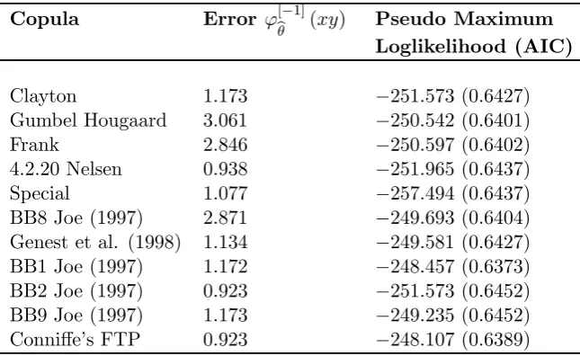
In our example, this value is 0.04 which is less than the 0.23 applying to the data in Luciano et al. (2008), demonstrating the lighter censoring. The empirical Kendall function has been derived from Dabrowska’s nonparametric estimator of the joint survival function (see Dabrowska, 1988). As an additional check, the pseudomaximumlikelihood (PML) procedure as in Genest et al. (1995) - with as input rescaled Kaplan Meier estimates of the marginal survival functions in order to accommodate censoring - has been employed for each candidate copula.
Copula Error [−1]
() Pseudo Maximum Loglikelihood (AIC)
Clayton 1173 −251573 (06427)
Gumbel Hougaard 3061 −250542 (06401)
Frank 2846 −250597 (06402)
4.2.20 Nelsen 0938 −251965 (06437)
Special 1077 −257494 (06437)
BB8 Joe (1997) 2871 −249693 (06404)
Genest et al. (1998) 1134 −249581 (06427)
BB1 Joe (1997) 1172 −248457 (06373)
BB2 Joe (1997) 0923 −251573 (06452)
BB9 Joe (1997) 1173 −249235 (06452)
[image:18.595.130.453.128.326.2]Conniffe’s FTP 0923 −248107 (06389)
Table 2: Results additional copulas.
Conniffe’s FTP and Genest et al. (1998), as well as their special cases of BB1, BB2, and BB9, and BB8 respectively. The results are given in Table 2. Akaike’s Information Criterion (AIC) has been added in parentheses.
When considering distance (column 2), Conniffe’s FTP effectively reduces to BB2, which performs best. In terms of pure PML value (column 3), Conniffe’s FTP gives the bestfit of all, although when adjusted for the number of parameters involved, BB1 could be preferred. The family 4.2.20 Nelsen which came out as a winner in Luciano et al. (2008) gives a good fit when minimum distance is used as criterion, but does not perform so well when looking at PML.
To conclude, while it is not so clear whether dependence between couples is to be increasing or decreasing over time, this example shows that Conniffe’s FTP - containing both BB1 and BB2 as special cases - is worthwhile to be considered as a candidate copula. In this specific case it outperforms the Genest et al. (2008) family.
7
Conclusions
In this paper, we have derived an Archimedean copula from a utility function in two different ways, which permits to determine the magnitude of dependence featured by the copula. Ordering copulas by means of the notion of “Happiness of Attaining Wealth 1” (1) and the very common Arrow-Pratt coefficient of relative risk aversion is straightforward. Relative risk aversion is a key measure that also gives information about the presence or absence of the properties Left Tail Decreasing or Right Tail Increasing, while it is directly related to Oakes’ cross ratio function. The three-parameter Archimedean copula model derived from the Flexible Three Parameter utility function by Conniffe (2007) is versatile and seems suited for many applications.
The connections identified are particularly useful for new utility families appearing in the literature. Information provided about risk aversion pertaining to such utility functions - usually reported at least through the coefficients of absolute and relative risk aversion - enable the actuary, risk manager or anyone adopting a copula model to judge on the appropriateness of the derived copula family. Suitable applications seem to apply in particular to risks with a time dimension, such as insurance contracts on two lives and credit risk.
This paper has focused on extracting copulae from utility functions. One could take the opposite route by deriving utility functions from Archimedean generators. We will leave this as a topic for future research.
Acknowledgements
The author would like to thank Iqbal Owadally, Vladimir Kaishev and Andreas Tsanakas for proof reading and providing useful feedback on previous versions of this paper. Thanks are also due to Elisa Luciano and Elena Vigna for helping with the numerical application. An anonymous referee is acknowledged for providing valuable comments.
References
[1] Arrow, K.J., 1971. Essays in the Theory of Risk-bearing. North-Holland Publishing Com-pany.
[2] Aumann, R.J., Kurz, M., 1977. Power and taxes. Econometrica 45 (5), 1137-1161.
[3] Avérous, J., Dortet-Bernadet, J.-L., 2000. LTD and RTI dependence orderings. The Cana-dian Journal of Statistics 28 (1), 151—157.
[4] Avérous, J., Dortet-Bernadet, J.-L., 2004. Dependence for Archimedean copulas and aging properties of their generating functions. Sankhy¯a 66 (4), 1-14.
[6] Charpentier, A. (2003). Dependence and tail distributions. Paper presented at the Seventh International Conference on Insurance: Mathematics and Economics.
[7] Colangelo, A., Scarsini, M., Shaked, M., 2006. Some positive dependence stochastic orders, Journal of Multivariate Analysis 97, 46-78.
[8] Conniffe, D., 2007. Theflexible three parameter utility function. Annals of Economics and Finance 8 (1), 57-63.
[9] Dabrowska, D.M., 1988. Kaplan-Meier estimate on the plane. The Annals of Statistics 16, 1475-1489.
[10] Esary, J.D., Proschan, F., 1972. Relationships among some concepts of bivariate depen-dence. The Annals of Mathematical Statistics 43 (2), 651-655.
[11] Foncel, J., Treich, N., 2005. Fear of ruin. Journal of Risk and Uncertainty 31 (3), 289-300. [12] Frees, E.W., Carriere, J.F., Valdez, E.A., 1996. Annuity valuation with dependent mortality.
Journal of Risk and Insurance, 63 (2), 229-261.
[13] Genest, C., Ghoudi, K., Rivest, L.P., 1995. A semiparametric estimation procedure of dependence parameters in multivariate families of distributions. Biometrika 82 (3), 543-552.
[14] Genest, C., Ghoudi, K., Rivest, L.P., 1998. Discussion on “Understanding relationships using copulas” by E. Frees and E. Valdez. North American Actuarial Journal 2 (3), 143-149.
[15] Genest, C., MacKay, J., 1986. Copules archimédiennes et familles de lois bidimensionelles dont les marges sont données. The Canadian Journal of Statistics 14 (2), 145-159.
[16] Hougaard, P. (1986). Survival models for heterogeneous populations derived from stable distributions. Biometrika 73 (2), 387-396.
[17] Joe, H., 1997. Multivariate Models and Dependence Concepts. Chapman & Hall.
[18] Jones-Lee, M.W., 1980. Maximum acceptable physical risk and a new measure of financial risk aversion. The Economic Journal 90, 550-568.
[19] Li, J., 2010. Fear of loss and happiness of win: properties and applications. Journal of Risk and Insurance 77 (4), 749-766.
[21] Luciano, E., Spreeuw, J., Vigna, E., 2008. Modelling stochastic mortality for dependent lives. Insurance: Mathematics and Economics 43 (2), 234-244.
[22] McNeil, A.J., Nešlehová, J., 2009. Multivariate Archimedean copulas, d-monotone functions and 1-norm symmetric distributions. The Annals of Statistics 37 (5B), 3059-3097.
[23] Merton, R.C., 1971. Optimum consumption and portfolio rules in a continuous-time model. Journal of Economic Theory 3, 373-413.
[24] Müller, A., Scarsini, M., 2005. Archimedean copulae and positive dependence. Journal of Multivariate Analysis 93, 434-445.
[25] Nelsen, R.B., 2006. An Introduction to Copulas, second edition. Springer.
[26] Oakes, D., 1989. Bivariate survival models induced by frailties. Journal of the American Statistical Association 84 (406), 487-493.
[27] Pratt, J.W., 1964. Risk aversion in the small and in the large. Econometrica 32 (1-2), 122-136.
[28] Saha, A., 1993. Expo-power utility: a flexible form for absolute and relative risk aversion. American Journal of Agricultural Economics 75, 905-913.
[29] Spreeuw, J., 2006. Types of dependence and time-dependent association between two life-times in single parameter copula models. Scandinavian Actuarial Journal (2006), 286-309. [30] Spreeuw, J., 2010. Relationships between Archimedean copulas and Morgenstern utility functions. In: Jaworski, P., Durante, F., Härdle, W.K., Rychlik, T. (Eds.) Copula Theory and its Applications - Proceedings of the Workshop Held in Warsaw 25-26 September 2009, Chapter 17, 309-320.
[31] Sungur, E.A., 2002. Some results on truncation dependence invariant class of copulas. Com-munications in Statistics-Theory and Methods 31 (8), 1399-1422.
[32] Wang, W., Wells, M.T. (2000). Model selection and semiparametric inference for bivariate failure-time data. Journal of the American Statistical Association 95, 62-72.
[33] Xie, D., 2000. Power risk aversion utility functions. Annals of Economics and Finance 1, 265-282.