A unified mixed-integer programming model for simultaneous fluence weight and aperture optimization in VMAT, Tomotherapy, and Cyberknife

A Unified Mixed-Integer Programming Model for

Simultaneous Fluence Weight and Aperture

Optimization in VMAT, Tomotherapy, and CyberKnife

Kerem Akartunalı

Department of Management Science, University of Strathclyde, Glasgow, G1 1QE, United Kingdom, [email protected]

Vicky Mak-Hau

School of Information Technology, Deakin University, Burwood, Vic 3125, Australia, [email protected]

Thu Tran

Andrew Love Cancer Centre, Barwon Health, Geelong, Vic 3220, Australia, [email protected]

In this paper, we propose and study a unified mixed-integer programming model that

simul-taneously optimizes fluence weights and multi-leaf collimator (MLC) apertures in the

treat-ment planning optimization of VMAT, Tomotherapy, and CyberKnife. The contribution of

our model is threefold: i. Our model optimizes the fluence and MLC apertures

simultane-ously for a given set of control points. ii. Our model can incorporate all volume limits or

dose upper bounds for organs at risk (OAR) and dose lower bound limits for planning target

volumes (PTV) as hard constraints, but it can also relax either of these constraint sets in

a Lagrangian fashion and keep the other set as hard constraints. iii. For faster solutions,

we propose several heuristic methods based on the MIP model, as well as a meta-heuristic

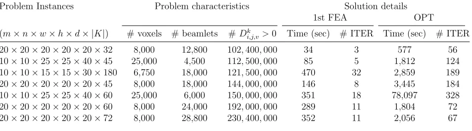
approach. The meta-heuristic is very efficient in practice, being able to generate dose- and

machinery-feasible solutions for problem instances of clinical scale, e.g., obtaining feasible

treatment plans to cases with 180 control points, 6,750 sample voxels and 18,000 beamlets

in 470 seconds, or cases with 72 control points, 8,000 sample voxels and 28,800 beamlets

in 352 seconds. With discretization and down-sampling of voxels, our method is capable

of tackling a treatment field of 8000 cm3 ∼ 64000 cm3, depending on the ratio of critical structure versus unspecified tissues.

Key words: OR in medicine; Integer programming; Heuristics; Radiotherapy treatment

1.

Introduction

Radiation therapy or radiotherapy has become one of the most common treatment methods

for cancer, besides chemotherapy and surgery, with almost two-thirds of all cancer patients

expected to have radiotherapy at some stage in their treatment plan [11]. In this treatment,

high-energy radiation is used to shrink tumors and kill cancer cells, where radiation damages

the DNA of cancer cells [17]. The radiation can be delivered either by radioactive source(s)

placed in or near the tumor, called brachytherapy; or by a machine outside the body, called

external radiation therapy, the most common form of radiotherapy. Since our focus is external

radiotherapy, we will refer to that simply as radiotherapy in the remainder of the paper.

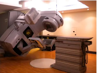
Figure 1: Gantry that can rotate by 360 degrees.

In radiotherapy, radiation beams are produced by a Linear Accelerator (LINAC), aimed

towards the tumor and its surrounding tissues where cancer may have spread. The LINAC is

mounted on a gantry, and the gantry rotates the source of radiation beams around the body

of a patient. Volumetric-modulated arc therapy (VMAT), Tomotherapy and CyberKnife are

recent major advances in external beam radiotherapy.

In VMAT, the gantry can rotate around a patient’s body by 360◦ in a co-planar manner

(see Figure 1). Co-planar treatments are possible through rotation of the LINAC couch.

or Varian’s RapidArc [32]). An “arc” does not necessarily have to be a full 360◦ rotation. In

Tomotherapy, the source of radiation will continuously rotate around the body of a patient

in a helical manner (see [2]), hence it is capable of delivering non-coplanar beams. In

CyberKnife, the source of radiation is mounted on a robotic arm, and therefore it can deliver

radiation beam from almost any point in space (see [1]). In addition to cancer treatment,

VMAT and Tomotherapy have also been used for Total Marrow Irradiation (TMI) in reducing

Leukemia relapse ratio (see [10] and [38]).

The modulation of the radiation beams is carried out using collimators. For VMAT, a

multi-leaf collimator (MLC) is mounted in the LINAC head. The MLC is made up of leaves,

which will block the radiation and are arranged parallel to each other in two sets of opposing

banks. These leaves can move independent from each other and can create customised beam

shape by positioning themselves in a planned position. The radiation field formed by the

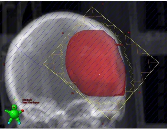
MLCs are known as aperture (see Figure 2). For example, if an aperture is formed by 20

leaves, each 1cm thick, and we have 20 leaf positions, then the MLC is said to have 400

bixels (or beamlets).

Figure 2: An MLC can form a shape that resembles the shape of the tumor.

On the other hand, TomoTherapy uses simply binary MLCs, i.e., each leaf has only two

eye view as per Figure 2. CyberKnife has various collimators, e.g., the M6 FI model uses

multiple circular collimators of different sizes (called IRIS collimators), whereas the M6 FM

model uses an MLC called InCise.

Since MLCs are common in all three machines, we focus our model on optimizing the

radiation intensity or fluence weight as well as the MLC aperture simultaneously. Some

MLCs do not allow interdigitation, that is, the left leaf of a row cannot collide with the right

leaf of the neighbouring rows, and vice versa. This is also known as the interleaf constraints

in the literature. Some MLCs allow full interdigitation, while some allow no interdigitation

or no interdigitation with a gap. There are also other machinery constraints for VMAT,

such as a limit to the speed a leaf can move in consecutive control points. Such a restriction

can be translated to the number of positions, or columns, a leaf is allowed to move between

control points before the MLC carriage shifts to enable further proximal/distal positions.

1.1

Recent developments in treatment planning optimization

To plan a radiotherapy treatment that involves the use of an MLC, one must decide from

where the radiation beams should be delivered, the intensity of radiation that should be

delivered from each location, and what apertures the MLC should form at those locations.

The general goals of a treatment is: i. for tumors to receive enough radiation so that they

can be eliminated, ii. for organs at risk (OARs) to be spared from radiation as much as

possible for minimal damage to healthy tissue, and iii. for the overall treatment time to be

as short as possible for patient’s comfort. The tumor area is usually given a margin that

will cover some surrounding tissues where cancer may have spread to and to compensate

for motion and setup. This area is called the Planning Target Volume (PTV). Before the

treatment planning optimization takes place, a radiation oncologist prescribes the dose limits

to the different structures: a lower bound on the dose to the PTVs (or a volume constraint

such as “at least 95% of the PTV must receive a dose of 73.7 Gray (Gy) or above”); and an

upper bound on the OARs (or volume limits such as “no more than 35% of the bladder can

receive more than 40 Gy of radiation”).

The question of where will be answered by a set of locations, commonly referred to as

the control points(CPs). The question of intensity at CP k is determined by the dose rate

(rk, in Monitor Unit (MU) per second), and the gantry speed (sk, also in MUsec). In recent

literature, e.g., [25] and [29, 30], a value calledfluence weightthat equals tork/sk is used for

what aperturethe MLC should form is where combinatorial optimization comes in. Further,

there is a limit in the maximum fluence weight that can be delivered from each control point.

For VMAT, the change in fluence weight is also limited in consecutive control points.

Notice that for all three treatment modalities, only one MLC aperture is considered

at each control point. On the other hand, in intensity-modulated radiotherapy (IMRT),

a widely used form of radiotherapy with machinery similar to VMAT, there are very few

control points (usually only 5-7) in each treatment, but multiple MLC apertures are used at

each control point.

Traditionally, fluence weights and MLC apertures are optimized separately. In IMRT,

three separate optimization problems are solved (see, e.g., [13], [8], and [7]). First, a

beam-angle optimization problem is decided. These angles are either predetermined by an

expe-rienced treatment planner or calculated by solving some optimization problems (see, e.g.,

[22, 35, 39]). The output is a number of angles (usually 5-7, at most around 10 for the most

complex cancer cases, i.e., head and neck) from where radiation is delivered. After that, a

fluence map optimization problem is solved [26], which will provide us with one intensity

matrix for each beam-angle (control point). Finally, a realization problem is solved to find

the right MLC apertures that will decompose the intensity matrices, and to find the most

time-efficient way to do so ([18]). The field of minimizing treatment times for the

step-and-shoot MLC radiotherapy practically began with the work of [36]. The most recent advances

in the minimizing of total treatment time can be found in [5, 18, 31].

Since the underlying mathematical problem for the VMAT is different, methods developed

for the IMRT cannot be directly applied to the VMAT. The difference mainly stems from

the interconnectivity between different control points and the computational complexity due

to higher degree of freedom in VMAT, as noted by [37]. To our knowledge, the treatment

planning optimization of the VMAT has rarely been studied in the field of mathematical

programming/operations research, although the problem offers interesting challenges. The

most recent treatment planning optimization algorithms can be found in [25] (a greedy

heuristic) and [29, 30] (a hybrid nested partitioning heuristic). On the other hand, recent

years have seen a growing interest from medical physicists: [6, 24, 20] propose various

heuris-tics for handling dose limits as soft constraints, whereas [34] propose a two-stage algorithm

using shortest paths and [23] extend a one-stage algorithm originally proposed for IMRT

problems. We refer the interested reader to [37] for an excellent review discussing detailed

an invaluable discussion comparing different therapies for different cancer cases.

In [25], a mixed-integer nonlinear programming model is presented. The method iterates

between two optimization problems: First, given a set of control points and their respective

MLC apertures, the fluence weights for all control points are optimized. Then, a column

generation approach is used to find the most promising control point and its associated MLC

aperture. The objective function used therein is to minimize the deviation of the calculated

dose from the prescribed dose. Hence, if the objective value of a solution is not zero, then it

means that there exist violations in dose limits. A down-sampled voxel grid is implemented–

one in every two voxels is sampled along each of the three dimensions in critical structures

and one in every four in unspecified tissues. The voxels are of size 4×4×2.5 mm3_{. Real} clinical cases were tested using GPU computing and solution times are shown to be very

fast. Computational results indicated that the dose constraints for most structures could be

reasonably satisfied except for the case with the bladder.

The methods of [29, 30], on the other hand, present a mixed-integer programming model

similar to the model presented in this paper. The variable sets are adopted from [16] for the

IMRT, allowing interdigitation and only enforcing the dose lower bound for PTV as hard

constraints. When solving the MIP problem, however, these constraints are relaxed in a

Lagrangian fashion in the solution methodology, and a generalized Benders decomposition

and hybrid nested partition method is used as the solution methodology. The authors present

the consecutive control point leaf movement constraint in their model, however, for a problem

instance we have tested, there seems to be violations of these constraints present. Their

algorithm is tested on 10 randomly generated non-clinical instances.

In CyberKnife, [27] presents a multi-criteria optimization approach to optimize the

flu-ence weights, solving linear programming problems in each step of the multi-criteria

opti-mization procedure, with dose constraints dualized in the objective function and solved by

a one-step Lagrangian relaxation with pre-determined dual multipliers.

In TomoTherapy, while there are publications in the optimization of treatment planning

parameters such as field width, pitch factor, and modulation factor (see, e.g., [28] and [12]),

to the best of our knowledge, there is no integer programming/combinatorial optimization

methods specifically designed for TomoTherapy treatment planning. It is, however, possible

to apply a VMAT treatment planning optimization method to helical tomotherapy. There

will be many more control points to consider, however, the MLC apertures are much easier,

1.2

Contributions of our paper

Our paper makes the following contributions to the radiotherapy treatment optimization

literature.

1. Both our MIP model and the meta-heuristic method optimizes the fluent weights and

the MLC apertures simultaneously. Most methods in the present literature either

op-timize only the fluence weights (using beam-eye-view as MLC apertures) or opop-timize

the two iteratively. Furthermore, our models involve the no-interdigitation (interleaf)

constraints, which can simply be removed if the MLC considered allows interdigitation.

With a simple modification of the interleaf constraints, our model can also

accommo-date the case of no interdigitation with a gap.

2. Our MIP model can be used as a quality analysis tool for existing heuristic algorithms,

as well as to confirm infeasibility of a specific patient’s case. Most of the existing

algorithms dualize the dose limits, reducing the problem to minimizing deviation from

prescribed dose limits. With a heuristic solution, even though computation times are

typically short (e.g., [25]), when the objective value does not return a zero, one can

never know whether the dose prescription is simply infeasible, or that the heuristic

method failed to find a solution that is dose-feasible. Our approach, on the other

hand, indicates clearly when a given dose prescription is simply infeasible.

3. Although our MIP model can currently solve problems of moderate size, advances in

optimization software, computer hardware, and parallel computing are taking place

rapidly, increasing the size of problems that can be tackled every day. We also

inves-tigate customized exact methods with better computational performance for our MIP

model in a companion paper [4]. Moreover, treatment planning often happens 2-3

weeks before the actual treatment is carried out, allowing time to extensively search

for a solution that is dose-feasible, rather than to provide a quick solution in a few

sec-onds that does not necessarily comply all dose requirements. As noted by Dr. Robert

D. Timmerman, vice chair of radiation oncology at the University of Texas

Southwest-ern Medical Center, radiotherapy plans will be significantly improved in the future,

“simply because current outcomes are unsatisfactory to patients” [11]. Therefore our

4. For faster solutions, we also provide several heuristic methods based on the MIP model,

as well as a meta-heuristic approach. With the meta-heuristic, we were able to solve

problems with up to 180 control points for a treatment field with 6,750 sample voxels

and 18,000 beamlets; and, in another instance, 72 control points with 8,000 voxels

and 28,800 beamlets, for which the first dose- and machinery-feasible solutions were

returned after 470 seconds and 352 seconds, respectively. Note that the sizes of

prob-lems we have tackled are comparable to those found in the literature, see, e.g., [25].

Using the same discretization and down-sampling of voxels used by [25], our method

is capable of optimizing a treatment field of 8000cm3 _{∼64000 cm}3_{, depending on the} ratio of critical structure versus unspecified tissues. Finally, any solution returned by

the heuristic will have neither violations to the prescribed dose nor violations to the

machinery restrictions.

1.3

Organization of the Paper

In Section 2, we will present an integer programming formulation of the problem, which

initially has non-linear terms but can be linearized with additional variables and constraints.

We will also discuss some valid inequalities that strengthen this formulation. In Section 3,

we will discuss the polyhedral properties of some key subproblems, and also the strength

of the inequalities presented in the previous section. We will present all proposed solution

methodologies in detail in Section 4, where we will also briefly discuss possible Lagrangian

relaxations of the problem. The empirical strength of these solution methods will be

in-vestigated extensively in Section 5. Finally, we will summarize our conclusions and address

potential future research areas in Section 6.

2.

A Mixed Integer Programming Formulation

In this section, we present a mixed integer programming formulation for the treatment

planning optimization of the VMAT.

2.1

Notation and Problem Description

In what follows, we consider a set of given control points. In the case of VMAT, one can

consider equally spaced partitions of the 360◦ coplanar space. For example, a 180 control

points can also be taken as equal partitions from the helical rotation. Even though there

will be more control points than VMAT if we are to consider fine partitions, there will be

significantly less leaf position combinations to consider. In the case of CyberKnife, one can

consider a given set of “promising” control points. In theory, one can have a large number

of such control points, but impose a limit in the number of control points with a non-zero

fluence weight. In this paper, we will consider only the case when a set of control points is

given. We now define some notation. Let:

- I ={1, . . . , m} be the index set of the MLC rows;

- J ={1, . . . , n} be the index set of the MLC columns;

- K ={1, . . . ,K} be the index set of control points;

- I×J be set of beamlets (or bixels), each cell (i, j) being a beamlet/bixel;

- J0 = {0, n+ 1} ∪J, with 0 and n+ 1 being the home positions of the MLC left and

right-leaves, respectively;

- δ be the maximum number of columns a MLC leaf is allowed to move in consecutive

control points;

- ∆ be the maximum amount of change in fluence weights that is allowed in consecutive

control points;

- V be the index set of all voxels;

- Vt be the set of voxels in the target volumes, i.e., tumor volumes;

- Vo be the set of voxels in the organs at risk (one can even define a set each for the

critical structures, e.g., VB for the set of voxels in the bladder(s));

- L={(`, r) | `, r∈J0, ` < r} be the set of feasible left- and right-leaf pairs;

- Dk

ijv be the beamlet-based dose deposition coefficient, i.e., the dose, at unit fluence

weight, received by voxelv from beamlet (i, j) in the interval defined by control point

k (this value can be pre-calculated in the manner as described in [25]);

- ¯d > Lv, for v ∈Vt be a desireddose for voxels in a PTV (e.g., we may have 73.7 Gy as

Lv and 79.2 as ¯d);

- Uv be the maximum dose allowed for any given voxel v ∈V;

- yk

i(`,r) ∈ {0,1} be a decision variable with yki(`,r) = 1 representing the bixels between, but not including, columns ` and r in row i in control point k are open;

- xv ∈ {0,1}be a decision variable with xv = 1 if voxelv ∈Vt receives a desired dose of

¯

d or above, and xv = 0 otherwise;

- dv be the dose that voxel v receives;

- zk _{be a continuous decision variable representing the fluence weight for control point}

k; and

- ¯M be the maximum fluence weight that can be delivered from any control point.

2.2

The Formulation

There are some machinery constraints that are common among VMAT, TomoTherapy, and

CyberKnife, and some constraints that vary among the three treatment modalities. For

VMAT and CyberKnife, some MLCs allow interdigitation, whereas others do not. With

TomoTherapy, since there are only two leaf positions for each leaf, interdigitation is not an

issue. With VMAT, there will be a maximum travel distance for the leaves in consecutive

control points. Moreover, a maximum fluence weight change is also limited. There are also

dose lower limit and upper (or volume) limit constraints. Hence, we propose the following

formulation that will capture most of the machinery constraints. We emphasize here that

a feasible solution to our model is dose- and machinery-feasible, and is therefore an overall

Formulation 2.1

maxf(x, y, z) (1)

s.t. X (`,r)∈L

yk_i,(`,r) = 1 ∀i∈I, ∀k ∈K (2)

n+1

X

˜

r=`+1

y_ik_(`,r˜)+

`

X

˜

r=1 ˜

r−1

X

˜

`=0

y₍k_{i+1)(˜`,r˜)} ≤1

∀i∈I\{m},∀`∈J0\{n+ 1},∀k ∈K (3)

r−1

X

˜

`=0

y_ik_(˜`,r)+

n

X

˜

`=r n+1

X

˜

r=˜`+1

y₍k_{i+1)(˜`,r˜)} ≤1

∀i∈I\{m},∀r∈J0\{0},∀k ∈K (4)

r−δ−1

X

˜

r=0

r−1

X

˜

`=0 yk+1

i(˜`,r˜)+

n+1

X

˜

r=r+δ+1 ˜

r−1

X

˜

`=0 yk+1

i(˜`,r˜) ≤1−y

k i(`,r)

∀i∈I, ∀(`, r)∈ L, ∀k∈K (5)

`−δ−1

X ˜ `=0 n+1 X ˜

r=˜`+1 yk+1

i(˜`,˜r)+

n

X

˜ `=`

+δ+1

n+1 X ˜ r= ˜ `+1 yk+1

i(˜`,˜r)≤1−y

k i(`,r)

∀i∈I, ∀(`, r)∈ L, ∀k∈K (6)

zk−zk+1 ≤∆ ∀k∈K (7)

zk+1−zk ≤∆ ∀k∈K (8)

dv ≥Lv v ∈Vt (9)

dv ≤Uv v ∈V (10)

dv ≥dx¯ v v ∈Vt (11)

x∈ {0,1}|Vt|

;y∈ {0,1}|I|×|L|

; 0≤zk≤M¯ (12)

We first discuss three possible objective functions. The first objective function is suitable

for cases where the dose prescription is feasible to be carried out–cases that a solution that

satisfy all lower and upper dose limits dose indeed exist. In real-life cases, this is of course

not known in advance, in which case the model can be used to prove that no feasible solution

exists.

1. With all dose restrictions as hard constraints, we first consider f(x, y, z) = P

v∈Vtxv,

i.e., we maximize the number of voxels in the PTV that receive a desired radiation of ¯

provide an equal weight for each voxel in the target area to receive a good dose, which

will favor dose homogeneity as advised in [15].

We also note that the xv variables can be used to model volume requirements. For

example, a requirement such as “at least 95% of PTV must receive a minimum dose

of 79.2 Gy” can be written as:

dv ≥ 79.2xv, ∀v ∈Vt

P

v∈Vtxv ≥ 0.95|Vt|.

On the other hand, a volume constraint such as “no more than 17% of the bladder can

receive 65 Gy or above” can be achieved in the following way. Let VB be the set of

voxels in a bladder,M a large number, we replace the objective function by minv∈VB xv

and include the following constraints:

dv−65 ≤ M xv, ∀v ∈VB

P

v∈VB xv ≤ 0.17|VB|.

In this case, the xv will be a penalty counter of the number of bladder voxels being

delivered a dose over 65 Gy. The next two objective functions are suitable for difficult

cancer sites where prescribed doses are known to be typically very hard to be satisfied.

2. Keeping only the PTV dose lower limit constraints (50) as hard constraint, we can

minimize the dose delivered to the OARs in the objective function, i.e., minP

v∈Vodv.

Alternatively, we can minimize the dose upper limit violations for voxels in OARs,

either min{maxv∈Vo{(dv −Uv)

+_{}} (highest violations) or min}P

v∈Vo(dv −Uv)

+ _(total violation). Note that a simple dose lower limit feasibility check can be performed prior

to solving the optimization problem, where if there exists any v ∈ Vt such that Lv >

¯

MP

k

P

i∈I

P

j∈JDkijv, then the dose prescription does not have a feasible solution.

3. Keeping only the OAR dose upper limit constraints (51) as hard constraint, we can

maximize the dose delivered to the PTV in the objective function, i.e. maxP

v∈Vtdv.

Alternatively, we can minimize the dose lower limit violations for voxels in PTVs,

i.e. min{maxv∈Vt{(Lv −dv)

+_{}} (highest violations) or min}P

v∈Vt{(Lv −dv)

+_{} (total} violation).

We now explain the rest of the constraints. Constraint (2) ensures that only one shape

is used for each control point. This applies to all three treatment methods. Constraints (3)

Rowi+ 1 cannot overlap with the left (right) leaf in Rowi. Here we note that although some

MLCs allow interdigitation (i.e., no interleaf constraints needed), the interleaf constraints

in general make the problem computationally harder and they cover a more general set

of problems; hence we include them in the formulation. We can easily remove them for

TomoTherapy and for MLCs that do allow interdigitation.

Constraints (5) and (6) require that MLC leaves do not move faster than δ columns

between successive control points, which applies to VMAT only. Similarly, for VMAT (and

potentially for TomoTherapy too), we have the constraints (48) and (49) that limit the

difference between fluence weights for consecutive control points to be at most ∆.

Constraints (50) and (51) ensure that the dose lower and upper bounds be satisfied, and

(52) determines whether the binary variablexv can take a value of 1, i.e., the dose applied on

voxel v is at least the desired minimum of ¯d. Finally, (53) indicates bounds and integrality

requirements of the variables.

The dose that a voxel receives, denoted by dv for each v ∈ V and calculated as in (13),

depends on both the MU delivered and the shape of the MLC at each control point:

dv =

X

k∈K

X

i∈I

X

j∈J



  

zk×D_ijvk × X

(`,r)∈L

`<j<r

yk_i(`,r)



  

(13)

In this form, the dose expression is nonlinear and not convex; therefore it would

compli-cate the problem significantly. Although some MINLP techniques could be used, it would

be more beneficial if an efficient linearization can be established. We first note that all the

nonlinear terms above are bilinear. Moreover, the zk_×Dk ijv ×

X

(`,r)∈L,`<j<r

y_ik_(`,r) terms are special that exactly one of the components is a binary variable and the other a continuous

variable. Therefore, we can define a new variable ¯zk

ij to indicate the MU amount for control

point k and beamlet (i, j) of the MLC, and hence redefine dv for each v ∈V linearly as

dv =

X

k∈K

X

i∈I

X

j∈J

¯

zk_ij×Dk_ijv (14)

Recall that ¯M is the maximum fluent weight that can be delivered from each control point.

(k, i, j) combination, that is, for all k ∈K, i∈I, j ∈J:

¯

z_ijk ≤M¯ X

(`,r)∈L

`<j<r

y_ik_(`,r) (15)

¯

z_ijk ≤zk (16)

¯ z_ijk ≥M¯



  

−1 + X

(`,r)∈L

`<j<r

y_ik_(`,r)



  

+zk (17)

¯

z_ijk ≥0 (18)

SinceP

(`,r)∈L,`<j<ryki(`,r)∈ {0,1}, the variable ¯zijk will be forced to zero when

P

(`,r)∈L,`<j<ryki(`,r)= 0, and to zk when P

(`,r)∈L,`<j<ry k

i(`,r) = 1. Note that this linearization corresponds to Mc-Cormick’s envelope [19] and is known to give the convex envelope for general bilinear terms.

Substituting the linear dose definition (54) into the constraints (50)-(52) and adding the

above constraints, the problem is defined as: zV M AT = max{(1)|(x, y, z,z¯) ∈ XV M AT},

where XV M AT ={(2)−(53),(55)−(58)}.

Given the variety of objective functions and constraints one can study, in this paper,

we have chosen to study the combinatorial optimization problem precisely as stated in

For-mulation 2.1, where the first objective function is used, i.e., maxP

v∈Vtxv. We also note

that we have developed and performed preliminary test on a formulation adopted from the

model of [16] for IMRT, wherein for each control point and each row, three sets of variables,

(tk_ij, `k_ij, r_ijk ∈ {0,1}n_{), are used to represent the aperture, witht}k

ij = 1 if bixel (i, j) of control

point k is open, `k_ij = 1 if bixel (i, j) is occupied by the left leaf, and r_ijk = 1 if bixel (i, j)

is occupied by the right leaf. (In our model, we need (n+ 2)(n + 1) y-variables to do the

same job). The leaf logic constraints and the interleaf constraints are presented in [16]. We

derived our own consecutive control point leaf movement constraints. From our

prelimi-nary experiments on the MIP-based heuristics, however, the performance of the Langer-type

model is faster in some cases, but slower in others. It finds better objective values (P

vxv) in

some cases, but worse objective values in others. A table will be presented in the numerical

results section with further discussion. Based on these preliminary results, we decide to use

our own formulation presented in this section for further analysis and experiments. The full

2.3

Improving the Formulation: Valid Inequalities

In this subsection, we improve the above formulation by considering stronger inequalities

that would replace some of the original constraints, and present numerical results to show

the strengths of these inequalities. The number of tightened inequalities is equal to the

number of original constraints and therefore we will benefit from these inequalities without

any obvious additional computational cost. Moreover, as discussed in the upcoming sections,

these inequalities are facet-defining for some subproblems while providing computational

improvements.

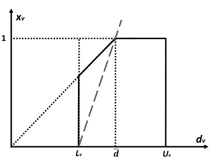
Proposition 2.1 The following inequality is valid and dominates (52).

dv−Lv ≥( ¯d−Lv)xv (19)

Lv Uv

dv

xv

1

𝒅

Figure 3: Geometric view of (19) (dashed line) vs. (52) (dotted line starting from the origin)

Note that if Lv = 0 holds for any v ∈ V, (19) becomes equivalent to (52). The effect of

these strengthened inequalities can be seen in Figure 3 with respect to original constraints

(52), when Lv > 0. The proof of this proposition is straightforward and is hence omitted

here. The following notation is used frequently in the rest of this section.

Definition 2.1 The cumulative demand from column ` to column r is given by: Dk i,`,r,v =

Pr

j=`D k ijv.

Proposition 2.2 For allk ∈K, i∈I, j ∈J, the inequality

zk−z¯_ijk ≤ X

(`,r)∈L

`≥jW

r≤j

min{M ,¯ min

v∈V

Uv

Dk

i,`+1,r−1,v

}yk_i(`,r) (20)

Proof. First of all, note that due to constraint (2), we have:

X

(`,r)∈L

`≥jW

r≤j

y_ik_(`,r)= 1− X

(`,r)∈L

`<j<r

y_ik_(`,r), ∀k∈K, i∈I, j ∈J.

If, for any given (`, r) ∈ L such that ` ≥ j or r ≤ j, yk

i(`,r) = 1, then ¯z

k

ij = 0, and zk ≤ Uv

Dk

i,`+1,r−1,v

has to be satisfied due to (51). On the other hand, if for any given (`, r)∈ Lsuch

that ` < j < r, y<sub>i</sub>k<sub>(`,r)</sub> = 1, then ¯z_ijk =zk. Therefore, (20) is valid. As min{M ,¯ Uv

Dk

i,`+1,r−1,v

} ≤

¯

M, (20) dominates (57). 2

Corollary 2.1 For all k ∈K, i∈I, j ∈J, the inequality

¯

z_ijk ≤ X

(`,r)∈L

`<j<r

min{M ,¯ min

v∈V

Uv

Dk

i,`+1,r−1,v

}y_ik_(`,r) (21)

is valid for the VMAT problem and dominates (55).

The corollary can be proven similar to Proposition 2.2 and hence we omit the proof.

Proposition 2.3 The following are valid inequalities for the VMAT problem:

(a) For i∈I, j, j0 ∈J, k ∈K:

¯

z_ijk −z¯_ijk0 ≤

X

(`,r)∈Ls.t. (`<j<r) V

(j0_≥rW

j0_≤`)

min{M ,¯ min

v∈V

Uv

Dk

i,`+1,r−1,v

}yk_i(`,r) (22)

(b) For i, i0 ∈I, j, j0 ∈J, k ∈K:

¯

z_ijk −z¯_ik0_j0 ≥



  

X

(`,r)∈L

`<j<r

min{M ,¯ min

v∈V

Uv

Dk

i,`+1,r−1,v

}yk_i(`,r)



  

−M¯ (23)

The proof of the second inequality is similar to the proof presented on p.82 of [33] and

hence omitted here. The proof of the first inequality is straight forward due to the fact

that ¯z_ijk ≤ min{M ,¯ minv∈V _Dk Uv i,`+1,r−1,v

} and hence omitted here. Note that the first set of

We conclude this section with a remark: we run preliminary computational tests to see

if and how the inequalities discussed in this section would make a difference. We tested

the strengths of the inequalities (19)- (23) individually added to the LP relaxation of the

original formulation, as well as the effect of adding all these inequalities together. These

results indicated that constraints (19) provide by far the most significant improvement to

the LP relaxation bound. The improvements made by (21) and (22) were observed to be

mild, and ones made by constraint (20) and (23) were very insignificant. Therefore, we

simply replaced (52) with (19) and will use this formulation in the remainder of the paper

for all the methods that are based on MIP.

3.

Assumptions and Polyhedral Analysis

In this section, we study the polyhedral structure of the MIP. First, we list our assumptions

for the model that ensure the model to be both realistic and also non-trivial for the studied

cases:

• P

k∈K,i∈I,j∈JM D¯ k

ijv ≥ Uv, ∀v ∈ V. Otherwise, we can set Uv =

P

k∈K,i∈I,j∈JM D¯ k ijv.

Note also that from the practical point of view (with realistic number of control points

and size of MLC discretization matrix) P

k∈K,i∈I,j∈JM D¯ k

ijv >> Uv.

• d¯≤ Uv, ∀v ∈ Vt. Otherwise, xv = 0 and the variable can be eliminated from the

problem. To keep problem instances more interesting, we further assume ¯d < Uv.

• Lv < d¯, ∀v ∈ Vt. Otherwise, with the current objective function, xv = 1 will hold in

any feasible solution.

• Lv >0 and Dijvk >0, ∀k∈K, i ∈I, j ∈J.

Note that the last assumption is only necessary for the following discussion, in order to ensure

that the studied polytopes are non-trivial (e.g., when Dk

ijv = 0, one can simply eliminate

this bixel (i, j) from the problem; on the other hand, havingLv = 0 would allow the trivial

solution of “origin”).

Next, we will look at subproblems that can be analytically studied but can also be

extended to other crucial subproblems and hence provide important insight. We use the

points, and v voxels. We also note that we will omit any indices that have only a single

element for the sake of easier readability.

3.1

A Study of the

P

Polytope

Using our notation, P1×n×|K|×1 represents the convex hull of the model with a single row, n columns, |K| control points, and a single voxel. In the following discussion, the indices

for rows and voxels will be omitted. For MLCs that allows interdigitation, the interleaf

constraints can be removed, resulting in single row subproblems. From an analytical point

of view, a model with a single voxel captures the basic settings for the optimization problem,

where one is to make decisions on MLC apertures and fluence weights for each control point.

Hence, our polyhedral study of the P1×n×|K|×1 polytope will provide us with insights on inequalities that are promising for the general model with multiple voxels. The notation

Dk `,r =

Pr

j=`D k

j for k ∈ K will be used throughout this section. Also, note that |L| =

(n+1)(n+2)

2 . In what follows, for simplicity, we use L to representLv, as there is only a single voxel.

Proposition 3.1 dim(P1×n×|K|×1) =|K||L|+n|K|+ 1, when M D¯ k1,n ≥L for each control

point k ∈K, and |K| ≥4.

Proof. First, note that there are |K||L|+n|K|+|K|+ 1 variables (the y/¯z/z/x variables,

respectively) and |K| equations, hence dim(P1×n×|K|×1) ≤ |K||L|+n|K|+ 1. In order to show dim(P1×n×|K|×1)≥ |K||L|+n|K|+ 1, we list the following |K||L|+n|K|+ 2 affinely

independent points, where > 0 is a sufficiently small number and ∃¯k,kˆ ∈ K with ¯k 6= ˆk.

We choose an arbitrary τ ∈ {0, . . . , n}. We have the following three cases.

Case 1 We have altogether|K|+2 points with: yk

(τ,τ+1) = 1, for allk ∈K\{kˆ}; andy ˆ

k

(0,n+1) = 1;

Case 1a 1 solution with: zkˆ _{= ¯z}ˆk j0 = L

Dˆk (1,n)

, for all j0 = 1, . . . , n; and 0 otherwise;

Case 1b 1 solution with: zkˆ _{= ¯z}ˆk j0 = U

Dˆk (1,n)

, for all j0 = 1, . . . , n; x= 1, and 0 otherwise;

Case 1c 1 solution with: zkˆ _{= ¯z}ˆk

j0 = L+

Dˆk (1,n)

, for all j0 = 1, . . . , n and 0 otherwise;

Case 1d |K| − 1 solutions, one for each k ∈ K \ {ˆk}, with: zˆk = ¯z_jˆk0 = L

Dkˆ (1,n)

, for all

Case 2 There are |K|(|L| −1) points, one for each k ∈K and for each (`, r)∈ Lk

Lk =

L \ {(0, n+ 1)} if k= ˆk; and

L \ {(τ, τ + 1)} otherwise,

y₍k<sub>`,r)</sub> = 1 holds for (`, r)∈ Lk; yk

0

(τ,τ+1) = 1, for allk

0 _{∈K \ {k, β}, for β = ¯k if k = ˆk,}

otherwiseβ = ˆk;y₍₀β_,n+1) = 1, ¯z_jβ0 = L

Dβ_(1,n), for allj

0 _{= 1, . . . , n;z}β ₌ L

Dβ_(1,n), whereβ = ¯k

if k = ˆk, otherwise β = ˆk; and all other variables equal zero.

Case 3 We have n|K| points, one for each k ∈K and each j = 1, . . . , n, given as: yk

(j−1,j+1) = 1, z

k_{= ¯z}k j =

L nDk

j

; yβ_(0,n+1) = 1, for β = ¯k if k = ˆk, and β = ˆk otherwise; yk0

(τ,τ+1) = 1, for all k

0 _{∈K \ {k, β} for β = ¯k if k = ˆk, and β = ˆk otherwise;}

¯ z_jβ0 =

(n−1)L

nD₍₁β_,n), for all j

0 _{= 1, . . . , n; z}β ₌ (n−1)L

nDβ_(1,n), forβ = ¯k ifk = ˆk, andβ = ˆk otherwise,

and all other variables equal zero.

For k = ¯k, as we have ¯zk¯

j > 0, the only way to obtain this is through some linear

combination of other vectors with ¯z¯k

j >0. However, the only vectors with ¯z

¯

k

j >0 have

yˆk

(0,n+1) = 0, which will not give us y ˆ

k

(0,n+1) = 1 as needed. Hence these vectors are affinely independent to all of the previously introduced vectors. A similar justification

can also be made for the case ofk = ˆk. 2

Proposition 3.2 The following are the trivial facets ofP1×n×|K|×1, under the condition that

|K| ≥4 and other necessary conditions as indicated next to the constraints:

(a) x≥0;

(b) x≤1 when M D¯ k

(1,n)>d¯, ∀k∈K and d < U¯ ;

(c) y₍k<sub>`,r)</sub> ≥0, for allk ∈K, and all (`, r)∈ L; (d) z¯k

j ≥0, for all k ∈K and all j ∈ {1, . . . , n};

(e) z¯_jk ≤zk, for all k ∈K and all j ∈ {1, . . . , n}.

The proof for Proposition 3.2 is provided in the appendices for the sake of readability.

Next, we present key results regarding the inequalities presented in Section 2.3.

Proposition 3.3 The following are non-trivial facets of P1×n×|K|×1:

(b) zk_−z¯k j ≤

X

(`,r)∈L

`≥jW

r≤j

min{M ,¯ Uv Dk

`+1,r−1

}y₍k_`,r).

Proof.

(a) As we need to satisfy that dv =Lv when xv = 0, and dv = ¯dwhen x= 1, we can reuse

the vectors presented in the proof of Proposition 3.1 with the following modifications:

We remove the vector presented in Case 1(c), and in Case 1(b), we replace U by ¯d.

(b) We use again the vectors presented in the proof of Proposition 3.1 as a starting point.

First, note that we need to construct vectors that satisfy:

zk−z¯_jk = X

(`,r)∈L

`≥jW

r≤j

min{M ,¯ U Dk

`+1,r−1

}yk_i(`,r). (24)

Most of the vectors presented in Proposition 3.1 satisfies (24), unless noted in the list

of modifications presented below. Equation (24) is satisfied under three cases, which

we call as Case (α), Case (β), and Case (γ).

Case (α): We have yk

(`,r) = 1, for ` < j < r, in which case the right hand side of (24) equals zero. This means that either we have zk _{= ¯z}k

j = 0 (which appear in Case 2 of

the proof of Proposition 3.1); or zk = ¯zk_j =λ, for λ 6= 0, (which only happens in Case

3 of Proposition 3.1 withyk_j−1,j+1 = 1, and we have zk= ¯z_jk = _nDLk j

).

Case (β): We have yk

(`,r) = 1, for j ≤ ` or j ≥r, and r =`+ 1. In this case, ¯z

k j = 0,

and the right hand side also equals zero. In all but one case presented in the proof of

Proposition 3.1 that concern such yk

(`,r), we have z

k _{= ¯z}k

j = 0. The only vector with

suchy₍k<sub>`,r)</sub> and withzk6= ¯z<sub>j</sub>k appears in Case (1d) of the proof, where (`, r) = (τ, τ+ 1), zk 6= 0, but ¯z_jk= 0. We simply remove this vector.

Case (γ): We have yk

(`,r) = 1, for j ≤ ` or j ≥ r, and r > `+ 1. Again, ¯z

k

j = 0. In

the proof of Proposition 3.1, these cases appeared twice, once in Case 2, and once in

Case 3 in the proof of Proposition 3.1. The vectors all have ¯zk

j = 0. We simply change

the value ofzk _{from their original value assigned in the respective cases in the proof of}

Proposition 3.1 to zk = min{M ,¯ _DkU `+1,r−1

}. 2

3.2

The Special Case of

P

We now present our results on a number of non-trivial facet-defining constraints for the

unlikely to be an insightful subproblem for VMAT, but it is more insightful for IMRT, and

is therefore included in the paper for the sake of completeness. In the following discussion,

the indices for rows, control points and voxels will be omitted. For ensuring feasibility, we

simply exclude closed leaf positions from the following discussion, i.e.,L:=L\{(j, j+ 1)|j =

0, . . . , n}. Let D`,r =

Pr

j=`Dj. Note that the results presented in the previous section are

still valid and hence not repeated here.

Proposition 3.4 The inequality

z−z¯j ≥

X

(`,r)∈L

`≥jW

r≤j

L D`+1,r−1

y`,r (25)

is valid for P1×n×1×1 and dominates (56). Moreover, it is facet-defining for P1×n×1×1 under

the general condition of M D¯ _j00 > L, ∀j 00

∈J.

The following proposition concerns constraints that involve two columns, any arbitrary

dis-tinct columns).

Proposition 3.5 The 2-column inequalities for P1×n×1×1:

1. The 2-column inequality with j <bj,

¯

zj+ ¯zbj −z ≤

X

(`,r)∈L

`<jV b

j<r

min{M ,¯ U D`+1,r−1

}y`,r

− X

(`,r)∈L

`≥bjW

r≤jW

(`≥jV

r≤bj) L D`+1,r−1

y`,r (26)

is valid for P1×n×1×1, and is facet-defining under the general condition M D¯ j00 > L,

∀j00 ∈J.

2. The 2-column inequality with j <bj,

¯

zj+ ¯zbj −z ≥

X

(`,r)∈L

`<jV b

j<r

L D`+1,r−1

y`,r

− X

(`,r)∈L

`≥bjW

r≤jW

(`≥jV

r≤bj)

min{M ,¯ U D`+1,r−1

}y`,r (27)

is valid for P1×n×1×1, and is facet-defining under the conditions that M D¯ j00 > L,

4.

Solution Methodologies

In this section, we introduce four heuristic solution methods. We first discuss three natural

ways to obtain Lagrangian relaxations to the original MIP. We then explain why only two

of them are implemented in Sections 4.2 and 4.3. The third heuristic is based on a different

MIP-formulation of the model, and the last heuristic is based on the metaheuristic idea

of Variable Neighborhood Search, where we derive some problem-specific features to guide

the search. We note that customized exact methods for our MIP model are studied in a

companion paper [4].

4.1

Lagrangian Relaxation (LR) for Upper Bounds

Here, we consider three variants:

1. Relax constraints (3),(4), (50)-(51), (55)-(58): As proven by Proposition 4.1, the subproblem is guaranteed to be solved in polynomial time.

2. Relax constraints (5)-(52): This creates K separate subproblems, one for each control point k (each subproblem being an IP problem).

3. Relax constraints (55) and (57): This relaxation generates two subproblems, one for y variables and one for z and xvariables.

Let LRi indicate the Lagrangian Relaxation and LDi be the optimal solution of the

Lagrangian dual for i= 1,2,3, i.e.,

LDi = min

u x,y,z,max¯zLRi(u, x, y, z,z¯),

where u is the vector of Lagrangian multipliers.

Proposition 4.1 LD1 = max{(1)|(2)−(52),(55)−(58),0≤x≤1|Vt|,0≤y≤1|I|×|L|}. In words, optimizing the Lagrangian dual for the first relaxation will generate a bound equal

to LP relaxation of the original problem.

Proof. For this subproblem, consider the following network: For each i∈I, draw a network

withK+ 2 levels as follows: Level 0 has a single, dummy source node with supply of 1, level

K+ 1 has a single dummy sink node with demand 1, and each of the otherK levels have L

draw arcs to all L nodes in level 1. From level 1, draw arcs to level 2 in the way that MLC

shape (`, r) in level 1 can be changed to (`0, r0) in level 2. Repeat this for all levels until level

K is reached. Then, connect all the nodes in that level to the dummy sink node. It is easy to

observe that solving a shortest path problem through this network, where arc costs will be

de-fined as a combination of original objective function coefficients and Lagrangian multipliers,

will generate integral solutions toyvariables that satisfy the constraints (2),(5),(6). Finally,

note that constraints (52) are independent from previous constraints and there is only a single

binary variable on each constraint related to linear variables; therefore all extreme point

solu-tions will be integral. Therefore, conv({(x, y, z)|(2),(5),(6),(48),(49),(52), x∈ {0,1}Vt_{, y ∈}

{0,1}|I|×|L|_{}) = conv({(x, y, z)|(2),(5),(6),(48),(49),(52),0≤x≤1}Vt_,0≤y≤1|I|×|L|_}). 2

Since the Lagrangian dual for this relaxation does not provide a bound better than the

LP relaxation bound of the original problem, we do not investigate this further. However,

we make this technical comment for the sake of completeness.

Corollary 4.1 LD3 ≤LD1.

On the other hand, forLD2 and LD3, the subproblems do not in general produce naturally integer solutions, hence the Lagrangian dual bounds they generate will be at least as strong

as (or probably lower than) the LP relaxation bounds. Although, this may involve more

computational effort. As we will see in numerical results, LR2 is computationally cheap, whereasLR3 requires significant effort.

4.2

LR-Based Heuristic I

Our first heuristic is based on the control point independence feature of LR2. We relax machinery constraints that link the adjacent control points, i.e., (5)- (52), and are thus able

to solve each control point subproblem independently. Instead of penalizing all the violated

constraints in the objective function like the usual LR methods do, we penalize only the dose

violations (i.e., (50)-(51)), but “fix” the neighboring control point machinery constraints

((5), (6)) as follows. Once a single-control point subproblem is solved and its MLC shape

is determined, i.e., y-variables are fixed, we can impose the machinery constraints for the

neighboring control points. This is done iteratively until all MLC shapes for all control points

are obtained. Then, the problem reduces to a simple IP without machinery constraints (it

would have been simply an LP if constraint (52) was not included). Algorithm 1 provides

Algorithm 1 A heuristic that exploits control points consecutively, generating |K| candidate solutions.

1: fork∈K do

2: Solve the problem P1: min{P

v∈Vt(Lv−dv)

+₊P

v∈V(dv−Uv)+|(y, z,z¯)∈Xrel}

3: where Xrel={(2)−(4),(53),(55)−(58)}, for onlyk;

4: Solutions are fixed y-variables =⇒ MLC-shape for control pointk;

5: for k0=k+ 1. . .|K|and k0 =k−1. . .1do

6: Solve the problem P1’: min{P

v∈Vt(Lv−dv)

+₊P

v∈V(dv−Uv)+|(y, z,z¯)∈Xrel0 }

7: whereX_rel0 ={(2)−(49),(53),(55)−(58)}, for only k0;

8: Fix shapes for k0;

9: end for

10: Now all shapes fixed, solve the original problem;

11: end for

When we minimize the objective function in the inner loop, we involve all control

points that are fixed so far, in addition to k0, in order to minimize the error function

P

v∈Vt(Lv −dv)

+ ₊P

v∈V(dv −Uv)+ more accurately and to obtain more involved fixing

decisions. Also note that one can replace this objective function with a discrete function

that counts infeasibilities, i.e., minP

v∈Vtw −

v +

P

v∈V w

+

v such that w

−

v, wv+ ∈ {0,1} and

Lvw−v ≥Lv−dv; ( ¯MP_k∈K

P

i∈I

P

j∈JD K

ijv)w+v ≥dv−Uv. This will simply provide an equal

weight for each voxel to satisfy their dosage lower and upper bound constraints; rather than

the “error”. We believe that in theory, such a counting objective is appropriate, at least

mathematically, and is based on a similar logic like the objective function of our problem.

However, in a number of preliminary tests we ran, we have observed that this discrete

count-ing function does not behave well computationally possibly due to symmetry, and therefore

we use the original error function in the final algorithm.

In the current implementation, once the problem P1 is solved for k, first the forward

(i.e., for k0 = k + 1 to k0 = |K|) and then the backward (i.e., for k0 = k −1 to k0 = 1)

subproblems are solved. Forward and backward subproblems can be solved separately in

parallel at the same time if needed for a faster result, although we consider in this paper

the sequential time for fair comparison purposes and leave parallelization to future research.

We also note that one can apply different running orders of subproblems in the inner loop to

obtain different solutions, e.g., in the alternating order (i.e., k0 =k+ 1, k0 =k−1, . . . , k0 =

K, k0 = 1) or in a randomized order (i.e., pick with probability p forward or probability

1−p backward subproblem). We ran some limited experiments on this aspect and did not

observe any significant difference. Hence we implemented the simple sequential order in this

computational performance of Algorithm 1 (in particular how often feasible solutions can be

found, solution qualities, and computation times) will be discussed in Section 5.

4.3

LR-Based Heuristic II

Our second LR-based heuristic is a combination of subgradient optimization and an

IP-heuristic, applied in an iterative fashion to the third Lagrangian relaxation (LR3). If we relax constraints (55) and (57) and assign multipliers αk

ij and βijk respectively to these two

sets of constraints, we obtain two separate subproblems as follows:

(P r.1) : max

x,z,¯z

X

v∈Vt xv +

X

k∈K

X

i∈I

X

j∈J

(β_ijk −αk_ij)¯z_ijk −β_ijkzk

s.t. (48)−(53),(56),(58); and

(P r.2) : max

y

X

k∈K

X

i∈I

X

j∈J

¯

M(αk_ij−β_ijk) X

(`,r)∈L

`<j<r

y_ik_(`,r)

s.t. (2)−(6).

Once these independent subproblems are solved individually, we perform subgradient

optimization by updating the multipliers using a stepsize θ described as follows:

αk_ij ←α_ijk +θ



  

¯

zk_ij−M¯ X

(`,r)∈L

`<j<r

y_ik_(`,r)



  

, and

β_ijk ←β_ijk +θ



  

( ¯M(−1 + X

(`,r)∈L

`<j<r

y_ik_(`,r)) +zk)−z¯k_ij



  

.

Every time the multipliers are updated, the solution to (Pr.2) is used to fix ally-variables

and then a simplified version of the original problem is optimized to obtain a heuristic

solution. This algorithm then iterates back to solving the two subproblems with the new

multipliers. The computational performance (in particular how often feasible solutions can

be found, solution qualities, and computation times) will be discussed in Section 5.

4.4

A Centering-Based Heuristic

The challenge with the original formulation is the vast number of the y variables, as these

“center” of an opening in a row lies, then one could simply definen binary variables for this

row instead of n2 _{binary variables (hence a significant reduction of problem dimension and} computational complexity), where these binary variables either indicate the left-leaf position

(if column position is smaller than center) or the right-leaf position (if column position is

bigger than center). In a heuristic fashion, one can extend this idea to the “center of an

opening” for a given control point, i.e., a column being chosen as the center column for all

rows (rather than defining a center column for each row). Such a intuitive approach has the

potential that one can solve this (probably easy) problem iteratively multiple times, e.g., by

using different centering schemes. The pseudocode for the proposed heuristic is presented in

Algorithm 2.

First, we define our notation and reformulate the problem for control point k. Let y` ij

(y_ijr) be binary variables for row i and column j, where y_ij` = 1 (yr_ij = 1) holds when the

left (right) leaf position is on column j. Let ˆck represent the predefined center column for

this control point k, i.e., it is taken as center column for all rows, and ˆ`i (ˆri) indicate the

processed control point). The reformulation is then as follows:

ˆ

ck

X

j=0

y_ij` = 1 ∀i∈I (28)

n+1

X

j=ˆck₊₁

y_ijr = 1 ∀i∈I (29)

dv =

X

i∈I

X

j∈J

¯

z_ijk ×Dk_ijv ∀v ∈V (30)

¯ z_ijk ≤M¯

j−1

X

j0₌₀

y_ij`0 ∀i∈I, ∀j ∈[1,ˆck] (31)

¯ z_ijk ≤M¯

n+1

X

j0_=j+1

y_ijr0 ∀i∈I, ∀j ∈[ˆck+ 1, n] (32)

¯

z_ijk ≤zk ∀k ∈K, ∀i∈I, ∀j ∈J (33)

¯

z_ijk ≥M¯ −1 +

j−1

X

j0₌₀

y_ij`0

!

+zk

∀i∈I, ∀j ∈[1,ˆck] (34)

¯

z_ijk ≥M¯ −1 +

n+1

X

j0_=j+1

yr_ij0

!

+zk

∀i∈I, ∀j ∈[ˆck+ 1, n] (35)

¯

z_ijk ≥0 ∀i∈I, ∀j ∈J (36)

y`<sub>ij</sub> = 0 ∀i∈I, ∀j ∈J0\{`ˆi−δ,`ˆi+δ} (37)

yr_ij = 0 ∀i∈I, ∀j ∈J0\{ˆri−δ,rˆi+δ} (38)

One important aspect that needs further elaboration is the selection of ˆck _{for each control}

point k. We propose the following intuitive possibilities:

ˆ ck₁ =

X

v∈Vt Lv



  

X

i∈I

X

j∈J

(j−0.5)Dk_ijv

X

i∈I

X

j∈J

D_ijvk



  

X

Algorithm 2A centering-based heuristic, generating |K|candidate solutions.

1: Pre-solve to obtain ˆck for each control point k∈K;

2: fork∈K do

3: Using ˆck, solve the problem: min{P

v∈Vt(Lv−dv)

+₊P

v∈V(dv−Uv)+|(y`, yr, z,z¯)∈Xref}

4: where Xref ={(28)−(36)}, for only Control pointk;

5: Fix shapes for k, set ˆ`i and ˆri values;

6: for k0=k+ 1. . .|K|and k0 =k−1. . .1do

7: Using ˆck0, solve the problem: min{P

v∈Vt(Lv −dv)

+₊P

v∈V(dv −Uv)+|(y`, yr, z,z¯) ∈ X_ref0 }

8: whereX_ref0 ={(28)−(38)}, for only k0;

9: Fix shapes for k0, set ˆ`i and ˆri values;

10: end for

11: Now all shapes fixed, solve the original problem;

12: end for

ˆ ck₂ =

X

v∈Vo

1 Uv



  

X

i∈I

X

j∈J

(j−0.5)(1/Dk_ijv)

X

i∈I

X

j∈J

(1/Dk_ijv)



  

X

v∈Vo

1 Uv

ˆ

ck₃ =w1cˆk1 +w2ˆc

k

2

The value ˆck

1 emphasizes higher dose and lower Lv, and depends on only tumor voxel

parameters whereas the value ˆck

2 emphasizes lower dose and higher Uv, and depends only on

sensitive tissue parameters. ˆck

3 simply combines these two with weightsw1, w2. We observed minimal differences on some preliminary computational tests using different weights, hence

we use ˆck₃ with w1 = 0.5 = w2 in the final algorithm.

The main advantage of this framework is not only a significant reduction in the number of

variables but also in the elimination of inter-leaf constraints. On the other hand, this method

has the disadvantage that it limits the candidate opening patterns for a control point to only

“centered” patterns (e.g., the pattern cannot be diagonally-shaped) and infeasibilities are

more probable. We will discuss these aspects in detail in Section 5. We also note that

this heuristic is related to the first LR-based heuristic, where single-control point-problems

are solved consecutively for each control point, after the MLC apertures for the previous

control points are fixed. The main difference here is that the subproblem is even further

significantly. We will compare computational results for both of these methods in the next

section.

Finally, we also note that one might use this approach in an exact fashion, where the

pa-rameters ˆck _{will need to be redefined as variables. This will require a sophisticated approach}

using a specialized branch-and-bound and column generation scheme, which is investigated

thoroughly in a companion paper [4].

4.5

A Guided Variable Neighborhood Scheme (GVNS)

Our Guided Variable Neighborhood Scheme (GVNS) aims to tackle problems of large scale,

and therefore, feasibility is the primary objective; the first attempt is to obtain solutions

that satisfy all machinery and dose constraints. When such a feasible solution is found,

a pre-determined number of attempts to improve the original objective function will be

triggered. This is done by keeping track of the current best feasible solution with the highest

original objective value. If there are no improvements to the original objective value after

a predetermined number of dose and machinery-feasible solutions are found, we return the

current feasible solution with the best original objective value as an output.

The method randomly generates fluence weights and MLC shapes that satisfy the

ma-chinery constraints for each control point. We define two main neighborhoods:

• Nµ _{is the neighborhood of solutions obtained by modifying the fluence weights. This}

is further divided into N₊µ (increase MU by ∆µ) and N−µ (decrease MU by ∆µ).

• Ns _{is the neighborhood of solutions obtained by modifying the MLC shapes.}

For the former, we further define N±µ1 ⊂ N

µ

±2 ⊂ · · · ⊂ N

µ

±V N Smax, i.e., N

µ

±i is the

neigh-borhood defined by having i MUs increased (or decreased) while satisfying the machinery

constraints. (In our experiments, we used ∆µ = 1). V N Smax denotes the maximum number

of MUs that are allowed to be changed, calculated as a fraction of |K|.

Similarly, we also have N₁s ⊂ N₂s ⊂ · · · ⊂ N_{V N S}s _max, with N_ps representing the random selection of p control points and modifying the associated MLC shapes by moving each leaf

by a random selection from the feasible moves of the leaves. Our preliminary experiments

indicated that the result of implementing two different shape change schemes (enlarge shape

and reduce shape) does not differ significantly from that of the random shape change. With

the former, while fixing violations in underdosed voxels, overdose is often induced in other

• Method 1 - Random Descent Local Search

In this method, the neighbour search alternates between MU change (Nµ_{) and shape}

change (Ns_{). The method randomly selects a control point and modifies its MU or}

shape.

• Method 2 - A Guided Search

This is done in a way that the neighborhood search is “guided” by the current

solu-tion to improve machinery constraint satisfacsolu-tion. LetoCN T be the number of voxels

overdosed and uCN T be the number of voxels under-dosed. Then:

– if oCN T_{oCN T}−uCN T ≥0.1, we search the neighborhood of N₋µ₁to decrease the MU; – if uCN T_{uCN T}−oCN T ≥0.1, we search the neighborhood of N₊₁µ to increase the MU; – otherwise we search NS _{to change the shape.}

• Method 3 - A Variable Neighborhood Search

In this method, we also alternate between MU change and shape change. First, we

calculate V N Smax =dγ|K|e, for 0< γ <1 a user-determined value (we used γ = 0.3 in our experiments). Initially, we set size V N S = d|oCN T_|V−uCN T_| | ×(V N Smax −1)e. If there is no improvement to the objective value, we increase size V N S by 1, until

V N Smax is reached.

Method 3 is executed in two different ways. In Method 3a, shape change is carried

out when the iteration count is even with size V N S control points changed at a time,

and MU change is carried out otherwise. In Method 3b, in each iteration of the

neighborhood search, MU change and shape change are executed iteratively.

• Method 4 - A Guided Variable Neighborhood Search

Our preliminary results showed that Method 4 outperformed Methods 1–3, hence we

will describe only this method in details. The VNS and its variations have been

around for many years (for general literature overview, see [14, 21]). In our

problem-specific implementation, we modified the VNS by integrating the “guided search” idea

of Method 2.

We begin with a randomly generated machinery feasible solution with leaf positions

delivered to each voxel to find out the dose violations, and perform a search guided in

the manner of promoting dose satisfaction.

The objective function is given by vCN T = oCN T +uCN T. If vCN T > 0, the

GVNS will proceed to search for “neighboring” solutions by using one of the two

neighborhood search schemesNµ_andNs_{. Our method attempts to increase or decrease}

MUs in the first instance. We also perform MLC shape change on a regular basis, or

if no consecutive-control point-feasible MU change is possible. Should there be no

machinery feasible leaf movements available, we modify our shape change procedure

by first selecting i control points randomly, select the left- and right-leaf positions for

the first row of the MLC of each of these i control points, and generate leaf positions

for subsequent rows that satisfy the inter-leaf constraints. It is possible that some

consecutive control point leaf restrictions are violated, and these violations are added

into the cost function. Once in a while, a new MLC-feasible solution will be generated

for all |K| control points, allowing random starts for the search. See Algorithm 3 for

the pseudocode. We note the key notation, as follows:

– ItCN T a counter for number of iterations the GVNS has been performed.

– ItM AX a predetermined maximum number of iterations to be performed.

– ItN EW a new machinery feasible solution is generated everyItN EW iterations.

– κ a counter for the number of occurrences when a feasible solution is found and it does not improve the current best original objective function value.

– κmax the maximum value forκ allowed in the GVNS (in our experiments, κmax= 5).

– ω(x0) the value of the original objective function given by solution x0.