Quantized Census for Stereoscopic Image Matching

City, University of London Institutional Repository

Citation:

Slabaugh, G. G., Basaru, R. R., Child, C. H. T. and Alonso, E. (2015). Quantized

Census for Stereoscopic Image Matching. Paper presented at the Second International

Conference on 3D Vision (3DV 2014), 08-12-2014 - 11-12-2014, Tokyo, Japan.

This is the accepted version of the paper.

This version of the publication may differ from the final published

version.

Permanent repository link:

http://openaccess.city.ac.uk/id/eprint/4760/

Link to published version:

Copyright and reuse: City Research Online aims to make research

outputs of City, University of London available to a wider audience.

Copyright and Moral Rights remain with the author(s) and/or copyright

holders. URLs from City Research Online may be freely distributed and

linked to.

City Research Online:

http://openaccess.city.ac.uk/

[email protected]

Rilwan Remilekun Basaru

School of Informatics City University London London, United Kingdom

[email protected]

Chris Child, Eduardo Alonso, Greg Slabaugh

School of Informatics City University London London, United Kingdom

[email protected]@city.ac.uk

[email protected]

Abstract—Current depth capturing devices show serious drawbacks in certain applications, for example ego-centric depth recovery: they are cumbersome, have a high power requirement, and do not portray high resolution at near distance. Stereo-matching techniques are a suitable alternative, but whilst the idea behind these techniques is simple it is well known that recovery of an accurate disparity map by stereo-matching requires overcoming three main problems: occluded regions causing absence of corresponding pixels; existence of noise in the image capturing sensor and inconsistent color and brightness in the captured images.

We propose a modified version of the Census-Hamming cost function which allows more robust matching with an emphasis on improving performance under radiometric variations of the input images.

I. INTRODUCTION

Stereo-matching for disparity recovery has been used in a wide range of applications, including object recognition, object tracking, robotic navigation and even recovery of

landscape topography from aerial photography [11]. This broadness of scope implies that a good correspondence matching system has an inherent need to be adaptive to different illumination conditions. Basic stereo-matching systems utilise a simple matching cost function to identify corresponding points in images taken from multiple perspectives (often two) with the assumption of identical intensity level at points of corresponding image locations. We will refer to this as the Consistency Assumption. As a result of different illumination conditions, amongst other factors, the consistency assumption rarely holds and more complex cost functions are required to account for radiometric differences.

As mentioned above, several conditions breach the consistency assumption. The illuminating conditions are a major issue as they can seldom be controlled. This is as a result of non-Lambertian surfaces and specular reflection [5]. The difference in illumination to the light sensor component of the cameras will result in the same point in 3D space being perceived at different intensity levels. Another cause of radiometric differences is the

inconsistency of the image capturing devices themselves. Properties such a salt and pepper noise, Gaussian noise, vignetting, gain setting (linear and non-linear) etc. will generally be inconsistent in multiple devices hence resulting in radiometric differences. Whilst pre-calibration is a good remedy to these problems, it could be quite tedious and the solution would only be partial. Hence developing accurate cameras for stereo-matching often requires expensive techniques and resources.

The above discussion, establishes that the requirement for robustness against radiometric differences is essential for a stereo-matching system to be used in real application. In this paper we propose an improved Census cost function [3]. It is important to note that we have focused on the cost function rather than on the matching algorithm. Hence a basic window to window search is carried out and no further optimizations are integrated. Our key contribution in this paper is that we have generalized the Census cost function by incorporating a quantization term that improves its robustness to radiometric changes that do not preserve the relative ordering of pixel values whilst still handling gain or bias radiometric changes. As a result the proposed cost function (Quantized Census) is robust against different types of radiometric distortions. The rest of the paper is structured as follows: in the next section a survey of region-based matching cost functions is presented; section 3 introduces the proposed cost function; section 4 describes the dataset and experiments carried out; and section 5 discusses the results of the experiments. The paper is concluded and future work is discussed in section 6.

II. RELATEDWORK

Generally, region-based matching cost functions are of three categories, namely: Parametric, Non-Parametric and Mutual Information [6]. Common parametric matching cost functions include: Sum of Absolute Differences (SAD), and Sum of Squared Differences (SSD) each with a Locally-scaled and Zero-mean version - Locally-Locally-scaled Sum of Absolute Differences (LSAD), Zero-mean Sum of Absolute Differences (ZSAD), Locally-scaled Sum of Squared Differences (LSSD) and Zero-mean Sum of Squared Differences (ZSSD). Another type of parametric matching-cost is Normalized-Cross Correlation (NCC), (with a Zero-mean version- ZNCC) [6]. Each of the cost function assumes an already rectified image pair with corresponding matching pixel only horizontally displaced in the other image.

SAD is arguably the simplest of the window-based cost functions. SAD relies heavily on the consistency assumption and is calculated by taking the sum of the absolute difference of all intensity levels between the pixels within a neighbourhood in the first image and those in a potentially matching neighbourhood in the second image. The cost function can be mathematically described as follow:

𝐶𝑆𝐴𝐷(𝐩, 𝐝) = ∑ 𝐪 𝜖 𝑁_𝒑|𝐼𝐿(𝐪) − 𝐼𝑅(𝐪 − 𝐝)| (1)

where a corresponding search is made for pixel, p in the left image; d denotes the number of pixel-shifts away from the pixel, p in the horizontal line; and q denotes a pixel within a neighbourhood around p, called Np.

SSD is similar to SAD except that the differences are squared before summation within the window. This additional step means that it requires slightly more computation than SAD. Formally,

𝐶𝑆𝑆𝐷(𝐩, 𝐝) = ∑ 𝐪 𝜖 𝑁𝒑{𝐼𝐿(𝐪) − 𝐼𝑅(𝐪 − 𝐝)}2 (2)

The locally-scaled variants of SAD and SSD attempt to compensate for bias gain by multiplying each pixel value in one of the two neighbourhoods to be compared by the ratios of the mean intensity value of both regions. The equations are as follows.

𝐶𝐿𝑆𝐴𝐷(𝐩, 𝐝) = ∑ {|𝐼𝐿(𝐪) −𝐼𝑁𝑃,𝐿 ̅̅̅̅̅̅̅̅ 𝐼𝑁𝑃,𝑅

̅̅̅̅̅̅̅̅𝐼𝑅(𝐪 − 𝐝)|} 𝐪 𝜖 𝑁_𝒑 (3)

𝐶𝐿𝑆𝑆𝐷(𝐩, 𝐝) = ∑ {𝐼𝐿(𝐪) −𝐼𝑁𝑃,𝐿 ̅̅̅̅̅̅̅̅ 𝐼𝑁𝑃,𝑅

̅̅̅̅̅̅̅̅𝐼𝑅(𝐪 − 𝐝)} 2 𝐪 𝜖 𝑁_𝒑 (4)

where the overbar denotes the mean.

NCC is the most computationally expensive of the parametric cost functions considered in this paper. The NCC derived from cross-correlation which is effectively the integration of the product of two signals. These signals would have an amplitude distribution about the zero level. The NCC employs normalization before to the Cross-Correlation step to ensure that the image intensity values (which are always positive) are distributed about the zero level. Formally,

𝐶𝑁𝐶𝐶(𝐩, 𝐝) =

∑ 𝐪 𝜖 𝑁_𝒑{𝐼𝑳(𝐪) ∗ 𝐼𝑹(𝐪 − 𝐝)}

√∑ 𝐪 𝜖 𝑁𝒑{𝐼𝑳(𝐪)2 } ∗ ∑ 𝐪 𝜖 𝑁𝒑{𝐼𝑹(𝐪 − 𝐝)2}

(5)

The zero mean variants, ZSAD, ZSSD and ZNCC, also attempt to account for a constant bias gain radiometric difference. They achieve this by subtracting the intensity value of each pixel within the window of interest by the mean of the window. Hence the transformation is as follows:

IT(p) = I (p) - 𝐼̅(𝐩) (6)

𝐼̅(𝐩) =_𝑛(𝑁1

𝐩)∑ 𝐪 𝜖 𝑁𝒑𝐼(𝒒) (7)

of parametric matching cost function for example MNCC which is an approximation of the NCC but with faster computation [13].

Non-parametric matching-costs are invariant to monotonic gray value changes. They rely solely on the relative intensity levels of pixels within region. This allows them to tolerate a large class of local and global radiometric changes [4]. The Rank function and Census function are two major types of non-parametric matching-cost functions. The Rank matching cost transforms the intensity level of each pixel to its intensity ranking within the neighborhood. This transformation is used as a correspondence match by computing the absolute difference. This is known to be sensitive to noise in textureless regions [10]. The Census function is discussed in Section 3.A.

The final category of matching cost function is mutual information. Statistically, mutual information measures the strength of association between two random variables. It conveys the amounts of instances in which two events are observed together in comparison to when not observed together. In terms of stereo image correspondence, the random variables are the pair of potentially matching pixels points. Egnal [9] proposed the method of using mutual information for local stereo correspondence. At each pair of neighborhoods a histogram is generated and used to compute the joint probability of the intensity levels in both neighborhoods. Another common variance of MI is HMI (hierarchical mutual information) [14]. This uses a coarse-to-fine technique, by scaling down the images and then gradually scaling up. Starting with a randomly allocated disparity map, the images are displaced and the cost is computed.

III. DEVELOPINGTHEPROPOSEDMETHOD

A. Census-Hamming Distance

The Census cost function is implemented as a non-parametric local transformation to the window of interest whilst the Hamming Distance is the similarity measure that utilizes the result of this transformation. Consider a local neighborhood Np with a center pixel p and intensity I (p). Assuming a rectified stereo pair, with a pixel, p in the left image, the corresponding pixel in the right image is p-d. For a single image(left or right) the intensity level of the center pixel is compared to that of surrounding pixels (denoted with q) within the considered neighborhood to generate “a bit string representing the set of neighboring pixels whose intensity is less than” or greater than I (p) [3]. Formally,

𝐼𝐶(𝐩) = 𝐹{𝐼(𝐪) > 𝐼(𝐩)} (8)

where F{ } is a Boolean function that returns ‘1’ if the input is true and ‘0’ otherwise. The binary result from (8) is

concatenated across all the pixels in the neighborhood. The Hamming distance between the transformed neighborhoods in both corresponding images is then computed. This is the number of bit-positions that are different in two bit strings [3]. The larger this value the more dissimilar the two neighborhoods in question. Whilst the Census-Hamming combination is a strong cost function against some radiometric changes, it has one major flaw in that it is not invariant to non-monotonic radiometric distortions. Consider a 1D, image region with 5 pixels shown in Fig. 2a.

53 99 100 102 135

(a)

53 101 100 99 135

(b)

Figure 2. Intensity levels of a 1D Image region before (a) and after (b) non-monotonic distortion

Here the Census transform for this region would be: [0 0 1 1]. If the image is distorted non-monotonically, the relative ordering of intensity level is lost, for example, as shown in Fig. 2b. This would result in a different Census transform of [0 1 0 1]. Even though the distortion was slight, this results in a 50% error.

Other variances of the Census cost function are [16] and [15]. The first utilizes the mean intensity of the window instead of the intensity of the center pixel in the neighborhood while the latter adds a relatively small number to the mean intensity before comparing with neighboring pixels.

B. Quantized Census (QC)

We proposed Quantized Census in an attempt to compensate for the deficiency in the Census matching cost. QC applies a less rigid system that accommodates for non-monotonic distortions to the ordered level of intensity.

Just like in the Census case, QC utilizes the comparative intensity of the middle pixel and the neighboring pixels, but is also sensitive to intensity gradient. It transforms the intensity level at each pixel within the neighborhood of interest to a quantized equivalent of the difference in the intensity value of the middle pixel to that of the surrounding ones. This does not only provide information on the order of relative intensity but also, to some extent the magnitude. Continuing with our previous notation, the transformation is as follows:

𝐷(𝐪) = 𝑄𝑁{𝐼(𝐪) − 𝐼(𝐩)} (9)

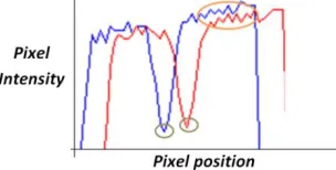
and +255 (intensity color range). For example if 16 bins were used, then the quantized value would range from -7 to 0 in the negative range and 0 to 7 in the positive domain. The effect of this equation is that subtle non-monotonic distortions, that do not preserve the order of pixel intensity, will not be detected by the cost function. This is significant as imaging devices would not perfectly capture subtle intensity changes in a scene. The 1D intensity row plot of a pair of stereo images shown in Fig. 3 illustrates this. It shows how the intensity of the pixels in the left image (red plot) and right image (blue plot) varies along an arbitrary row.

Figure 3. A 1D intensity row plot of the pair of the Tsukuba stereo image from the Middlebury dataset. [7]

Looking at the plot we can partially identify where some of the pairs of corresponding points are. However, we would also note that the relative ordering of intensity is not consistent especially in the low textured region. This will also be the case in the presence of distortions like Gaussian noise. Subtle intensity distortion due to Gaussian noise with low signal to noise ratio would be ignored as a result of quantization. For example, looking back at Fig. 2, if a quantized difference (with 16 bins) is applied then the resulting transform for both region A and B will be [-1 0 0 1]. Hence, it permits for the subtle non-monotonic distortion.

Whilst the modification in (9) has improved robustness, it immediately poses a problem. A key strength of the Census cost function is that it is robust to distortions like salt and pepper noise. It achieves this by not using an aggregative costing technique (in terms of intensity levels) like in SAD or NCC. Each erroneous pixel contributes equally to the cost, making it insensitive to outliers. With our modification, the intuitive cost would have been to acquire the sum of absolute or square differences. Of course this would be to the detriment of how well the cost function performs against outliers. This is because outliers that instigate huge quantized difference would influence the sum of absolute difference. Taking inspiration from the RANSAC algorithm [8], we used the number of outliers as opposed to summing the cost at each pixel. This has made the cost function invariant to radiometric changes that do not preserve the relative ordering of pixel values. Formally, we define the Quantized Census stereo-matching cost as

𝐶𝑄𝐶(𝐩) = ∑ 𝐹{|𝐷𝐿(𝐪) − 𝐷𝑅(𝐪 − 𝐝)| > 𝑇} 𝒒 𝜖 𝑁_𝒑

10)

where T is a threshold value. This cost is applied to the transformed neighborhood pair that is tested for correspondence. Here DL and DR refers to the quantized

pixel differences acquired by (10). To illustrate how (10) tolerates salt and pepper noise, consider a 3-by-3 region in a first image (region A in Fig. 4), and two potentially matching 3-by-3 regions in a second image (regions B and C in Fig. 4. These regions have been chosen to illustrate a linear gain scenario where the ground truth matching region is in fact region B with a bias of 30.

Figure 4. Intensity value of neighborhood

The resulting transformation (with 32 bins of quantization) for regions A, B and C will be.

Figure 5. Transformed values of neighborhood using (9)

First, note the invariance of the cost function to radiometric differences, while the relative pixel values are preserved. Next let us assume that the shaded pixel in region A is a randomly altered pixel value as a result of noise.

Figure 6. Resulting Cost when sum of the absolute difference of the transformed regions is used to compare Region A to Region B and C.

Fig. 6 illustrates the effect of the intensity level on the cost function had the sum of absolute difference been used instead of a threshold, as in (10). A significant degree of distortion in a single pixel is enough to affect the result of the cost function. If the intensity was distorted to less than 185, region C would wrongly be chosen as the best match. Instead, by considering the number of pixels pairs with absolute differences less than a particular threshold, this is rectified. In the above scenario, regardless of the intensity of the shaded pixel, the number of outliers will be the same.

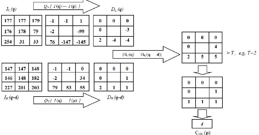
Fig. 1 gives a general flow diagram of Quantized Census. For a region in the first image and another potentially matching region in the second, the difference

0 2 4 6 8 10 12

0 _{16 32 48 64 80 96}

1

1

2

1

2

8

1

4

4

1

6

0

1

7

6

1

9

2

2

0

8

2

2

4

2

4

0

2

5

6

Su

m

of

D

if

fe

re

n

ce

Intensity of shaded pixel in Region A

Region B

between the intensity of the middle pixel and that of neighborhood pixels are acquired respectively. These differences are then quantized into an experimentally determined number of bins. In the case of Fig. 1, 16 bins were used. The absolute difference of the both transformed region is taking and the result is compared to a threshold (that is also experimentally determined) to generate a binary region. The sum of the binary region is to be minimized across all potentially matching regions.

IV. DATASET&EXPERIMENT

In the following experiment we compare the performance of QC and other cost functions in context of radiometric differences. We have not augmented cost functions with any smoothness, occlusion detection factors or any additional filtering. Hence we only evaluate the direct performance our cost against others. Both parametric cost and non-parametric cost functions were used. These included: SAD, LSAD, ZSAD, SSD, LSSD, ZSSD, NCC and Census. We use a simple window to window search algorithm on all of the cost functions. The search span of all cost functions was set to 10 pixels above the maximum disparity in the known ground truth.

Both synthetic and non-synthetic data sets were used in the experiment. The synthetic scene was generated using OpenGL. Here image pairs were captured from two

perspectives by displacing the synthetic camera

horizontally. This was particularly useful as it allowed the absolute disparity at each pixel to be computed from the baseline, FOV of the synthetic camera and the proximity of the scene to the camera by reversing the parallax equation. The non-synthetic dataset used were Teddy, Reindeer, Laundry, Art, Flowerpots and Cones from the Middlebury dataset [7] (Fig. 8). Each of the cost functions were trained using the synthetic data to determine the values of the parameters (such as window size, the threshold value and the quantization bin) that best optimized their performance. This ensured that the results indicated how well the cost functions were able to generalize, which is the key motivation for using Quantized Census. The data sets were altered to model five radiometric changes and the cost functions tested against these radiometric changes using implementation from [17]. These included a linear and non-linear distortion to the global intensity of the dataset; synthetized vignetting effect; Gaussian noise; and salt and pepper noise. Different levels of each distortion were used in the test. The linear and non-linear global intensity distortion; and the vignetting effect were applied to only one of the stereo image pairs while the Gaussian and salt and pepper noise were applied to both images in the pair.

All the tests and trainings were carried out on grayscale images. However the proposed cost method can easily be implemented for RGB data by, for example, applying the

transformation at each color channel and then

marginalizing to get the best match. For the evaluation, the

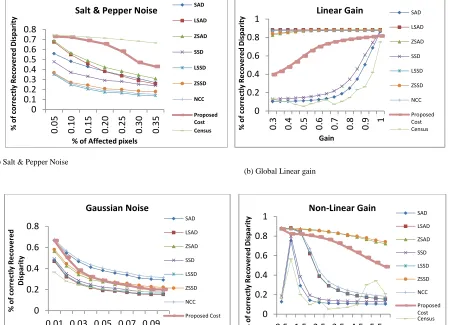
resulting disparity maps were compared against the ground truth by taking an absolute difference. A disparity value with an absolute difference error less than 1 pixel is considered to be right and vice versa. The Quantitative results are shown in Fig. 7, portraying the average percentage of rightly recovered disparity values over all six datasets. Occluded and non-occluded regions were not considered in the test as we only aim to compare relative performance. The resulting disparity for the Cone stereo pair is shown in Fig. 9.

V. RESULT&DISCUSSION

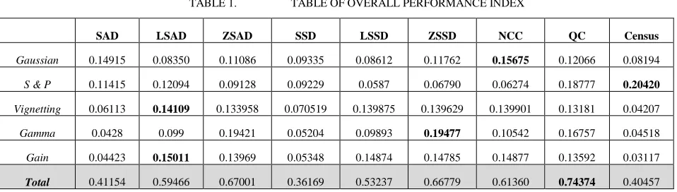
Based on the training results, QC’s performance was optimized with 16 bins of quantization at a threshold value of 2.These parameters, as well as a 3-by-3 window size were used in the previously described testing that followed. The results (Fig. 7) demonstrate how different cost functions are suited to specific radiometric differences. The locally scaled variants are theoretically suited for linear gain global distortion as the mean ratio explicitly counters this distortion. The same applies in the cases of: the NCC cost function in compensating for Gaussian; and Census in compensating salt and pepper noise. Quantized Census is able to generalize and be invariant to different types of radiometric changes. Although it does not outperform all other cost functions, it maintains a good performance across the different range of distortions. This makes it invaluable to the scenario where various radiometric distortions can exist - as is the case in most real-world applications. To illustrate the consistency of QC, an overall performance index has been computed across all the test results. This is shown in the table shown in Table 1. Here, for each radiometric distortion, the percentages of rightly recovered pixels are averaged and then normalized across each cost function. This provides an indication of the relative effectiveness of each cost function against the radiometric distortions. The overall performance index (in the bottom row of the table) is the sum of relative performance of each cost function across all the radiometric distortions. The performance index does not only indicate the superiority of QC over the other cost functions (in terms of consistency and generalization) but also the vast improvement that the proposed modification has made to the Census cost.

(a) Salt & Pepper Noise

(b) Global Linear gain

(c) Gaussian (White) Noise

(d) Non-Linear global gain

(e) Global Linear gain

Figure 7. Performance of the compared cost functions on Teddy, Laundry, Reindeer, Art, Flowerpots and Cones dataset. All plots show the percentage of rightly recovered disparity values by each cost function as different radiometric distortions are applied.

0 0.1 0.2 0.3 0.4 0.5 0.6 0.7 0.8 0.0 5 0.1 0 0.1 5 0.2 0 0.2 5 0.3 0 0.3 5 % of corr e ct ly R e cov e re d D is pari ty

% of Affected pixels

Salt & Pepper Noise SAD

LSAD ZSAD SSD LSSD ZSSD NCC Proposed Cost Census 0 0.2 0.4 0.6 0.8 1

0.3 0.4 0.5 0.6 0.7 0.8 0.9 1

% of corr e ct ly R e cov e re d D is pari ty Gain

Linear Gain SAD

LSAD ZSAD SSD LSSD ZSSD NCC Proposed Cost Census 0 0.2 0.4 0.6 0.8

0.01 0.03 0.05 0.07 0.09

% of corr e ct ly R e cov e re d D is pari ty Standard Deviation Gaussian Noise SAD LSAD ZSAD SSD LSSD ZSSD NCC Proposed Cost Census 0 0.2 0.4 0.6 0.8 1

0.5 1.5 2.5 3.5 4.5 5.5

% of corr e ct ly R e cov e re d D is pari ty Gamma Factor

Non-Linear Gain _SAD

LSAD ZSAD SSD LSSD ZSSD NCC Proposed Cost Census 0 0.2 0.4 0.6 0.8 1

0.1 0.2 0.3 0.4 0.5 0.6 0.7 0.8 0.9 1

(a) (b) (c) (d) (e)

(f) (g) (h) (i) (j)

Figure 9. Recovered disparity for the Cone pair without radiometric distortion applied: (a) SAD (b) LSAD (c) ZSAD (d) SSD (e) LSSD (f) ZSSD (g)NCC (h)QC (i) Census (j) Ground Truth

TABLE 1. TABLE OF OVERALL PERFORMANCE INDEX

SAD LSAD ZSAD SSD LSSD ZSSD NCC QC Census

Gaussian 0.14915 0.08350 0.11086 0.09335 0.08612 0.11762 0.15675 0.12066 0.08194

S & P 0.11415 0.12094 0.09128 0.09229 0.0587 0.06790 0.06274 0.18777 0.20420

Vignetting 0.06113 0.14109 0.133958 0.070519 0.139875 0.139629 0.139901 0.13181 0.04207

Gamma 0.0428 0.099 0.19421 0.05204 0.09893 0.19477 0.10542 0.16757 0.04518

Gain 0.04423 0.15011 0.13969 0.05348 0.14874 0.14785 0.14877 0.13592 0.03117

Total 0.41154 0.59466 0.67001 0.36169 0.53237 0.66779 0.61360 0.74374 0.40457

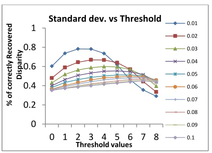
A. Threshold value Effect

In this section we explored how the performance of the QC cost function reacts to different levels of radiometric noise, as the threshold value chosen is altered. There was no significant relationship in the case of the linear and non-linear gain; vignetting; and the salt & pepper noise.

However, the Gaussian noise showed some correlation. Fig. 10 illustrates this relationship and in turn explains how the Quantized Census was able to compensate for Gaussian noise. As the standard deviation increases so does the optimum threshold value that produced the best result.

Figure 10. Performance of different threshold values for QC against different standard deviations of Gaussian noise

The threshold value implicitly determines the level of error the cost permits for when deciding what is conceded as a correct match. Subsequently, as the standard deviation (Signal-to-Noise) of the Gaussian noise increases the threshold value would need to increase to accommodate the increased error level.

VI. CONCLUSIONS

We have proposed, developed and evaluated an improved variant to the Census cost function, Quantized Census. A comparison has been made both experimentally and theoretically with other cost functions. The proposed cost function has been shown to have significantly improved performance of the Census cost function against different radiometric differences. Although Quantized Census does not outperform other cost functions against all distortions, it has proved to be the most consistent. This makes it more robust and more suited for real-world applications where different radiometric distortions appear.

As with every technique that employs some form of threshold or weighting there is an inherent disadvantage in having to decide the right threshold or weight to use. This is indeed the case with Quantized Census, with particular sensitivity to the threshold value. In future work we aim to propose and develop a technique of automatically selecting threshold values based on the intensity distribution in the scene. One approach would be to detect the level of noise in texture-less regions and alter the threshold accordingly.

REFERENCES

[1] A. Klaus, M. Sormann and K. Karner Segment-based stereo matching using belief propagation and a self-adapting dissimilarity measure. In International Conference on Pattern Recognition (ICPR), 2005.

[2] C. Fookes, M. Bennamoun, and A. Lamanna, “Improved stereo image matching using mutual information and

hierarchical prior probabilities,”in IEEE International Conference on Pattern Recognition, 2002.

[3] R.Zabih and J. Woodfill, “Non-parametric Local Transforms for Computing Visual Correspondence.” in Proceeding of the European Conference of Computer Vision. Stockholm, Sweden, May 1994, pp. 151-158.

[4] U. Stilla, F. Rottensteiner, H. Mayer, B. Jutzi, M. Butenuth “Photogrammetric Image Analysis” Springer, New York, pp160-161

[5] Oren, M. and S. K. Nayar, Generalization of the Lambetian model and implications for machine vision, Int.J.Comp. Vision 14, pp.227-251, 1995.

[6] Heiko Hirschmüller and Daniel Scharstein (2009), Evaluation of Stereo Matching Costs on Images with Radiometric Differences, in IEEE Transactions on Pattern Analysis and Machine Intelligence, Volume 31(9), September 2009, pp. 1582-1599.

[7] “Middlebury stereo website” [Accessed 9th _{June 2014].}

Available: http://vision.middlebury.edu/stereo/data/

[8] M. Fischler and R. Bolles, “Random Sample Consensus: A Paradigm for Model Fitting with Applications to Image Analysis and Automated Cartography,” Comm. ACM, vol. 24, no. 6, pp. 381- 395, June 1981.

[9] G Egnal “Mutual Information as a Stereo Correspondence Measure,” Technical Report MS-CIS-00-20, Uni. Of Pennsylvania, 2000.

[10]H. Hirschmüller and D. Scharstein (2007), Evaluation of Cost Functions for Stereo Matching, in Proceedings of the IEEE Conference on Computer Vision and Pattern Recognition, 18-23 June 2007, Minneapolis, Minnesota, USA.

[11]“Stereoscopy website” [Accessed 19th June 2014]. Available:

http://www.stereoscopy.com/faq/aerial.html

[12] “Image Synthesis website” [Accessed 29th _{June 2014].}

Available:

http://homepages.inf.ed.ac.uk/rbf/HIPR2/noise.htm

[13] H. Moravec, “Toward automatic visual obstatcle avoidance,” in Proceeding of the Fifth International Joint Conference on Artificial Intelligence, Cambridge, MA, August 1977, pp.584-590

[14] H. Hirschmuller, “Stereo processing by semi-global matching and mutual information,” in IEEE Conference on Computer Vision and Pattern Recognition, vol. 1, 2006, pp. 871-878. [15] Xin Luan, Honghong Zhou, Fangjie Yu, Xiufang Li, Bing

Xue, and Dalei Song: A robust Local Census-based Stereo matching insensitive to Illumination changes, Proc. of International conference on Information and Automation (ICIA), 2012.

[16] Froba, B., Ernst, A. “Face detection with the modified Census Transform,” In: Sixth IEEE International Conference on Automatic Face and Gesture Recognition. IEEE Computer Society Press, Los Alamitos (2004).

[17] “Siddhant Ahuja’s webpage” [Accessed 9th

June 2014] Available: http://siddhantahuja.wordpress.com/

0 0.2 0.4 0.6 0.8 1

0 1 2 3 4 5 6 7 8

% of

corr

e

ct

ly

R

e

cov

e

re

d

D

is

pari

ty

Threshold values

Standard dev. vs Threshold _0.01

0.02

0.03

0.04

0.05

0.06

0.07

0.08

0.09