University of Southampton Research Repository
ePrints Soton
Copyright © and Moral Rights for this thesis are retained by the author and/or other
copyright owners. A copy can be downloaded for personal non-commercial
research or study, without prior permission or charge. This thesis cannot be
reproduced or quoted extensively from without first obtaining permission in writing
from the copyright holder/s. The content must not be changed in any way or sold
commercially in any format or medium without the formal permission of the
copyright holders.
When referring to this work, full bibliographic details including the author, title,
awarding institution and date of the thesis must be given e.g.
AUTHOR (year of submission) "Full thesis title", University of Southampton, name
of the University School or Department, PhD Thesis, pagination
UNIVERSITY OF SOUTHAMPTON
FACULTY OF ENGINEERING, SCIENCE & MATHEMATICS
Optoelectronics Research Centre
Development and applications of dispersion controlled high
nonlinearity microstructured fibres
by
Ming-Leung Vincent Tse
Thesis for the degree of Doctor of Philosophy
UNIVERSITY OF SOUTHAMPTON
ABSTRACT
FACULTY OF ENGINEERING, SCIENCE AND MATHEMATICS
OPTOELECTRONICS RESEARCH CENTRE
Doctor of Philosophy
Development and applications of dispersion controlled high nonlinearity
microstructured fibres
By Ming-Leung Vincent Tse
In this thesis I investigate aspects of dispersion controlled high nonlinearity all silica holey fibre, including design, fabrication, sample applications, and modelling.
Microstructured fibre fabrication allows for great flexibility in core and cladding structure designs, with the large available refractive index contrast between glass and air. This allows the control of waveguide dispersion across a wide wavelength range, which can be used to offset the material dispersion of the core glass. Therefore, this technology provides improved overall dispersion control via fibre design. This often requires a complex arrangement of air holes in the structure.
The full fabrication procedures for small-core holey fibres are presented. In particular, the fabrication of fibres with a graded-hole-size structure is reported. A structural accuracy of ±6% is achieved and improvements are proposed for future work.
A systematic study of the Supercontinuum Generation phenomenon is presented in this thesis. By using fibres with different dispersion profiles, pumping at 1.06 μm, the nonlinear effects such as Self-Phase-Modulation, Four-Wave-Mixing and Self-Soliton-Frequency-Shift, which dominate the spectral broadening in fibres with one or two zero-dispersion wavelengths are identified accordingly.
ii
Contents
List of Figures v
List of Tables ix
Declaration of Authorship x
Acknowledgements xi
Abbreviations xii
1 Introduction 1
1.1 Holey fibre overview……….. 1
1.2 Guidance effects in microstructured optical fibres………. 1
1.2.1 Index guiding holey fibre………... 1
1.2.2 Guidance via photonic bandgap effects………. 2
1.3 Optical properties of index guiding fibres……….………. 3
1.3.1 Single mode operation ……….. 3
1.3.2 Large Mode Area and Highly Nonlinear Small Core fibres……….. 4
1.4 Thesis outline……….. 6
2 A review of nonlinear and dispersive effects in conventional and holey fibres 8
2.1 Introduction………. 8
2.2 Chromatic Dispersion……….. 9
2.3 Dispersion-induced pulse broadening……… 10
2.4 Nonlinearity……… 10
2.5 Generalised nonlinear Schrödinger equation………. 11
2.6 Propagation regimes……… 12
2.7 Stimulated Raman Scattering……….. 13
2.8 Self-Phase Modulation……… 14
2.8.1 Spectral Broadening………... 14
2.8.2 Self-Steepening……….. 15
2.9 Solitons……… 15
2.9.1 Introduction……… 15
2.9.2 Modulation Instability……… 15
2.9.3 Fundamental Soliton……….. 15
2.9.4 Higher Order Solitons……… 16
2.9.5 Soliton Preservation within optical fibres……….. 16
2.10 Split Step Fourier Method……….……….. 17
2.11 Nonlinearity and effective mode area in holey fibres………. 19
2.12 Dispersion management in holey fibres……….. 22
2.12.1 Shifts of zero-dispersion wavelength………. 22
2.12.2 Dispersion compensation………... 23
2.12.3 Dispersion-flattened designs……….. 23
2.12.4 Dispersion-decreasing designs………... 24
2.13 Loss mechanism……….. 24
2.13.1 Scattering loss………..………….. 25
2.13.2 Confinement loss……… 26
2.13.3 Bend loss………..………... 27
2.13.4 Coupling loss………. 28
iii
3 A guide to fabrication of small-core holey fibres 29
3.1 Introduction………. 29
3.2 Fibre draw tower………. 30
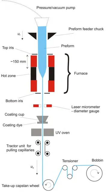
3.2.1 Feeder and furnace………. 30
3.2.2 Polymer fibre coating………. 32
3.3 Capillary preparation………... 32
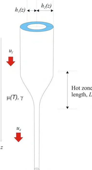
3.3.1 Analytical model for capillary drawing ……… 32
3.3.2 Capillary Drawing……….. 34
3.3.3 Capillary sealing and cleaning………... 36
3.4 Preform stacking………. 36
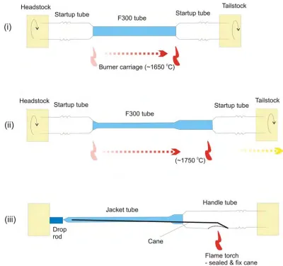
3.4.1 Jacket tube selection and preparation………. 39
3.4.2 Stacking techniques……… 39
3.4.3 Cleaning stacked preform……….. 38
3.5 Drawing canes from stacked preform.……… 40
3.6 Drawing fibre from canes……… 42
3.6.1 Jacket tube/preform preparation………. 42
3.6.2 Fibre drawing techniques... 43
3.7 Conclusions………. 44
4 Dispersion-flattened holey fibres 45
4.1 Introduction………. 45
4.2 Target designs………. 47
4.3 Fabrication of graded-hole-size fibres……….………… 47
4.3.1 Iteration one………... 47
4.3.2 Iteration two………... 51
4.3.3 Fibre analysis………. 53
4.4 Characterisation of graded-hole-size fibres……….……… 55
4.4.1 Chromatic dispersion measurement………... 55
4.4.2 Fibre loss measurement……….. 57
4.4.3 Birefringence measurement……… .. 57
4.4.4 Nonlinearity measurement………. 58
4.5 Tolerance analysis………... 59
4.6 Structural distortion investigation by varying fabrication techniques……… 61
4.6.1 Introduction……… 61
4.6.2 Old fibre drawing techniques………. 62
4.6.3 Secondary stacking techniques……….. 65
4.6.3.1 Stacking with rods……… 65
4.6.3.2 Stacking with capillaries………..… 67
4.6.4 Structure analysis……….. 68
4.6.5 Improved designs……….. 72
4.6.5.1 Three small holes design for 1 μm operation…….………... 73
4.6.5.2 A defected-core design……….………. 75
4.7 Conclusions………. 76
5 Dispersion-flattened fibres and supercontinuum generation at 1.06 μm 78
5.1 Introduction………. 78
5.2 Fibre designs………... 79
5.3 Fibre fabrications………. 82
5.3.1 Preform stacking……… 82
5.3.2 Jacket tube preparation……….. 83
5.3.3 Cane-in-jacket assembly……… 84
5.4 Fibre structure measurements & dispersion profiles……….. 86
5.5 Supercontinuum experiments……….. 95
iv
5.5.2 Experimental and numerical results……….. 96
5.6 Discussions……….... 99
5.6.1 Phase matching curves………. 99
5.6.2 Dominant nonlinear phenomena………....………….. 101
5.7 Conclusions………...… 106
6 Soliton compression at 1.06 μm in dispersion-decreasing holey fibres 107
6.1 Introduction………...… 107
6.2 Fibre design and fabrication...………...………… 108
6.2.1 Fibre design……….. 108
6.2.2 Fibre loss versus fibre length………...……… 111
6.2.3 Fibre fabrication & dispersion profiles……… 114
6.3 Soliton compression experiment………...… 116
6.3.1 Experimental setup………..……. 116
6.3.2 Experiment and Results……….... 117
6.4 Discussions………..……….. 121
6.5 Conclusions……….…….. 122
7 Designing tapered holey fibre for soliton compression 123
7.1 Introduction……….………….. 123
7.2 Fibre designs and contour map……….……. 124
7.2.1 Ideal adiabatic compression………. 125
7.3 Adiabatic compression in long fibres……….…….…….. 126
7.3.1 Minimised fiber length……….……… 133
7.4 Nonadiabatic compression……… 136
7.5 Compression in real fibres……….……… 137
7.6 Consideration of fibre fabrication………. 140
7.7 Conclusions.………..….... 143
8 Conclusions & Future work 144
8.1 Conclusions……….……….. 144
8.2 Future work………... 145
A Possible method to fabricate a graded hole-size fibre with pressure control for individual holes 147
List of publications 150
v
List of Figures
1.1 The typical structural arrangement of (a) a conventional optical fibre and (b) a typical
two-rings highly nonlinear holey fibre……….…..…………..2
1.2 A schematic of a typical structure of a photonic bandgap fibre………….………..3
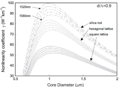
2.1 Nonlinearity coefficient as a function of the core diameter for a silica rod (dashed– dotted line), and the square lattice (solid line) and hexagonal lattice HF (dotted line) with d/L= 0:9; for each type, the characteristics of five wavelengths between 1520 and 1580 nm increasing in 15-nm steps are plotted, after reference [Hainberger, 2005]………..……….……….….. 20
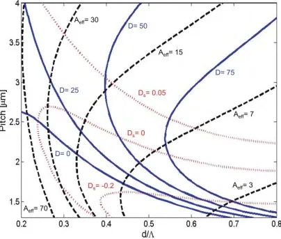
2.2 Contour map for dispersion (ps/nm/km), dispersion slope (ps/nm2/km) and effective area (μm2) versus pitch Λ and d/Λ for holey fibres of hexagonal geometry at 1.55 μm wavelength………...………..……….….…………...21
2.3 (a) Variation of dispersion with wavelength for HFs designed with different values of d/Λ when Λ= 1 μm, after reference [Saitoh, 2005(a)]. (b) Dispersion profiles against wavelength for three different HFs designed to have low-level ultraflattened dispersion, and the curve of a standard conventional single mode fibre, Corning SMF-28, after reference [Russell, 2006]………...…………...………..23
2.4 The loss versus core diameter of various holey fibres drawn from two preforms (A and B), with similar air-filling fraction, d/Λ> 0.9, after reference [Furusawa, 2003]………..……….…....26
2.5 Confinement loss for different air-filling fractions (left) and different number of rings of holes (right) as a function of Λ. The dotted line represents the loss of conventional fibers (0.2 dB/km), after reference [Finazzi, 2003]………....27
3.1 The schematic of the fibre draw tower………..…….….... 31
3.2 Definitions used for the analytical model of capillary drawing…………..……...…...33
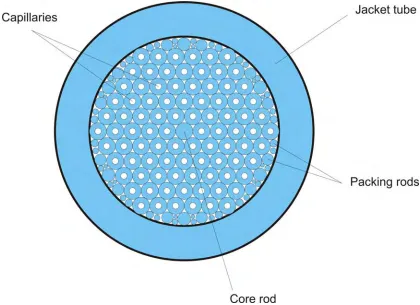
3.3 End view of the structural arrangement of a 5-ring holey fibre preform stack…...…..38
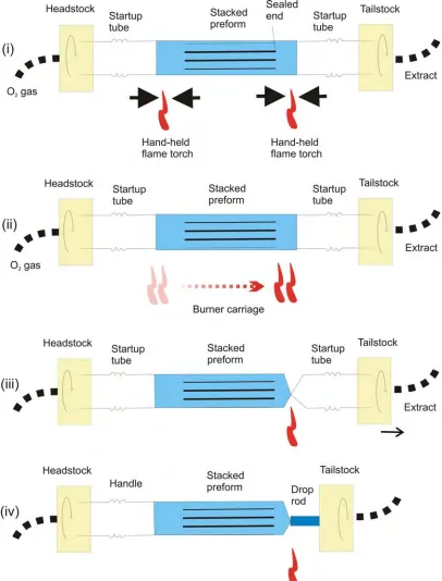
3.4 Step-by step schematics to show the procedures to clean a stacked preform………...39
3.5 (a) An image of a typical cane with a 7-rings structure taken under an optical microscope. (b) A SEM picture of a typical HNSC HF with 7 rings of holes…..…..…41
3.6 Step-by step schematics to show the procedures to stretch a 12 mm OD ‘F300’ tube into a jacket tube, and inserting the cane. ………...………..42
4.1 (a) Five-rings, dispersion-flattened HFs design with pitch Λ=1.58 μm and air-filling ratio d/Λ= 0.31, 0.45, 0.55, 0.63 and 0.95. (b) The predicted dispersion profile after reference [Saitoh, 2003]……….……….47
4.2 A structural image of the cane under an optical microscope in the transmission state...49
4.3 First iteration SEM micrographs of graded hole size HFs labelled ‘F426C’, ‘F456B’, ‘F467B’ and ‘F467C’ in chronological order………...…..50
4.4 (a) Average hole sizes and (b) average pitch sizes for each ring in the fibres…....……51
4.5 Second iteration SEM micrographs of graded hole size HFs………....….52
4.6 (a) Average hole size and (b) average pitch size for each ring in fibres ‘F573’ and ‘F585’...53
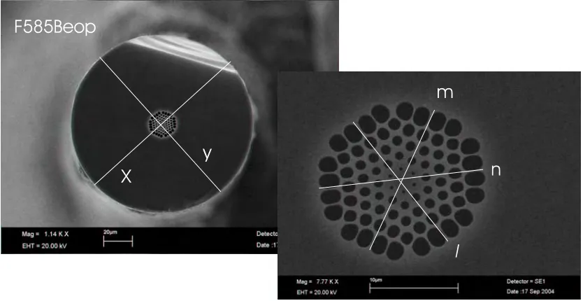
4.7 SEM micrograph of fibre ‘F585B’, indicates an elliptical fibre. x= 127.4μm, y= 124.6μm; ratio (1.02 : 1). m= 17.3 μm, n= 18.6 μm and l= 17.4 μm; ratio (1 : 1.08 : 1.01)……….…...…..……..54
4.8 (a) Optical microscope image of the cane from the second iteration. (b) Scale drawing of the capillary stack from the second iteration. (c) Overlay of (a) and (b)……….…...54
4.9 (a) Group delay + fitted curve (b) Chromatic dispersion profile of fibre ‘F467C’…...56
4.10 Dispersion profiles for ‘F426C’, ‘F456B’, ‘F467B’, ‘F467C’ and ‘F585C’…………..56
vi
4.12 A plot of the signal showing the polarisation beatings of fibre (a) ‘F426C’ and (b)
‘F585C’………..….58
4.13 Nonlinear phase shift verse output power with a linear fit for fibre ‘F456B’……..…..59
4.14 Modal information of the target design: (a) 1st higher order mode, (b) 2nd higher order mode, and (c) 3rd higher order mode……….…..60
4.15 Effect on the dispersion of error in (a) the pitch, and in (b) the first, (c) second and (d) third ring of holes. After reference [Poletti, 2005]………..…61
4.16 Cross-sectional arrangements of (a) Typical cane and jacket, (b) Cane, packing rods and jacket, and (c) Cane, packing capillaries and jacket……….……62
4.17 Jacket tube and cane setup with an additional neck on preform and simple stack in the holding tube……….….…...63
4.18 Schematics to show the vacuum collapse procedures for creating a jacket tube to fit the
cane………...…….…….64
4.19 Schematics to show the setup for jacket tube and secondary stacked cane with packing
rods………..…....66
4.20 SEM micrograph of fibre ‘F621’, (x : y) = (1.02 : 1) and (m : n : l) = (1.02 : 1.02 :1). Plus a optical microscope image of the cane used……….….67
4.21 Evolution steps of the microstructured region during the fibre draw of ‘F639’…….…68
4.22 (a) Average pitch size, (b) hole size, (c) d/Λ for each ring in fibres ‘F635’, ‘F621’ and
‘F639’……….…….71
4.23 The average percentage expansion of d/Λ during the cane-to-fibre process for different
fibres………72
4.24 (a) The schematic of the proposed 3 smaller holes structural arrangement, and (b) the corresponding dispersion. After reference [Poletti, 2007]………...……….……..73
4.25 A picture of the cane (top left), and the SEM picture of the 3-small holes fibre (‘F781’) and the corresponding feature size measurements for the first two rings………….…..74
4.26 (a) Schematic of the proposed dispersion-flattened structure. (b) The dispersion profile of the optimized design (dc/Λ= 0.279) and the corresponding profiles with a small
variation in the diameter of the defected central air-hole. After reference [Saitoh,
2005]………...75
5.1 Contour map for dispersion (units of ps/(nm km)), dispersion slope (ps/(nm2km)) and effective area (Shaded colour; μm2) versus pitch Λ and d/Λ for holey fibres of hexagonal geometry at 1.05 μm wavelength. (Dotted green line indicates single mode and multi mode boundary)………..………...….80 5.2 Dispersion graphs to show the tolerance levels of deviation in (a) d/Λ and (b) Λ from the optimum dispersion-flattened design. (Provided by F. Poletti)………....……81
5.3 The schematic of each element in the stack using the sleeve ‘Russian doll’ technique.82
5.4 Step-by-step schematics to show the procedures to stretch a 12 mm OD ‘F300’ tube into a jacket tube………...84 5.5 Schematic to show the cane-in-jacket assembly procedures………...…….….…..85
5.6 Schematic of the cane-in-jacket preform assembly (not in scale). Inset: Picture of the cane structure taken under an optical microscope in the transmission setting…………86
5.7 SEM micrographs of fibre ‘F738b’ at (a) SOP and (b) EOP……….….88
5.8 A Step-by-step guide to measure the hole positions and sizes using the ‘Scion Image’ program. (See text page 87 for a detailed description.)………...….…..89
5.9 The average (a) hole size, (b) pitch and (c) d/Λ of the first three rings along fibre ‘F738b’. (d) The calculated dispersion at 1.05 μm along the same fibre (Calculated by F. Poletti)………..….……..92
5.10 The calculated dispersion profiles at different point along fibre ‘F738b’ without the correction factor (Calculated by F. Poletti)……….…...……….93
5.11 Shows the drawing tool in ‘Scion Image’ for F738(b)sop with scale (Top) 27.5 pixels
vii
5.13 The SC spectra generated in Fibres A-F at different pump power levels…………..….97
5.14 The comparison of the simulated (blue, lower) and experimental (black, upper) spectra for (i) Fibre A, taken at 409 pJ in the experiment and 400 pJ in the simulation, (ii) Fibre D, taken at 251 pJ in the experiment and 240 pJ in the simulation, (iii) Fibre E, taken at 446 pJ in the experiment and 400 pJ in the simulation, and (iv) Fibre F, taken at 425 pJ in the experiment and 400 pJ in the simulation……….…………..……….98
5.15 The corrected dispersion profiles for Fibre A to F………..…..…… .99
5.16 Phase matching curves for Fibre A to E………...………....…100
5.17 The SC bandwidth (at maximum launched power) and the phase matched range for Fibre A to E………...……….…...100
5.18 The supercontinuum spectral evolution at increasing launched power in Fibre A..….102
5.19 The supercontinuum spectral evolution at increasing launched power in Fibre E...103
5.20 SC bandwidth at different input pulse energy levels for (a) Fibre A, and (b) Fibre E..105
6.1 Dispersion graphs to show the tolerance levels of deviation in (a) d/Λ and (b) Λ from the optimum dispersion-flattened design………..…110
6.2 (a) Simulation of pulse width along 10 m of DDHF with D= 10 to 1 ps/nm/km and 130 fs soliton input, and with different number of step increments. (b) Simulation of pulse width along 50 m of DDHF with D= 10 to 1 ps/nm/km and 380 fs soliton input, and with different number of step increments……….……111
6.3 Simulated output pulse width for different fibre lengths and losses with (a) D= 10 to 1 ps/nm/km, 380 fs input soliton, (b) D= 10 to 1 ps/nm/km, 130 fs input soliton, (c) D= 6 to 2 ps/nm/km, 130 fs input soliton………...………112
6.4 (a) The output pulse widths at different losses for the 10 m fibre length, D= 6 to 2 ps/nm/km (dotted line indicates 130 fs soliton input). (b) Shows the pulse widths along the fibre with loss=0, for 130 fs soliton and Gaussian inputs………...113 6.5 Soliton compression results for different input soliton widths in fibres with D= 6 to 2 at 1.06 μm, 11m in length, loss=0, where higher order dispersion effect is included…..114
6.6 Dispersion profiles used for numerical simulations for the input and output end of the fibre. Inset: SEM of the microstructure region of the fibre, and the dispersion at 1.06
μm along the fibre……….…115
6.7 Schematic of the experimental setup for pulse compression in DDHF…………...….116
6.8 (a) 3dB output pulse duration for different input pulse energies from experiment and simulations with an initial Gaussian pulse of 130 fs. The dashed curve shows the theoretical limit for adiabatic compression. Inset: the results taken from the other axis. (b) rms bandwidth from experiment and simulation……….……118
6.9 Left: Experimental (solid black line) and simulated (dotted green line) spectra (10 dBm/div.) at different input pulse energies. Right: Selected autocorrelation functions and pulse widths………119
6.10 3dB output pulse duration for different input pulse energies from experiment and simulations with an initial Gaussian pulse of 130 fs with different initial chirps….…120
6.11 Left: Simulated output spectrogram (logarithmic scale, time resolution = 0.1 ps) of a 3.5 pJ input pulse. Right: Spectrogram of a 63 fs soliton………..……….121
7.1 Contour map for dispersion (blue solid line; units of ps/(nm km)), dispersion slope (red dotted line; ps/(nm2km)) and effective area (black dashed line; μm2) versus pitch Λ and d/Λ for holey fibres of hexagonal geometry at 1.55 μm wavelength……….….…..…125
7.2 Contour map for adiabatic compression factors corresponding to the Fig. 8.1. (green dotted line represents the single mode ‘SM’ and multi-mode ‘MM’ boundary)……..126
7.3 Dispersion and effective area profiles along a 50 m fibre for (a) Path 1 and (b) Path 2 of Fig. 7.2. Inset: In both cases the fibre parameters Λ and d/Λ vary linearly along the fibre from (d/Λ= 0.20, Λ= 4.12) to (d/Λ= 0.27, Λ= 2.48)………....….128
viii
7.5 Simulated spectra at different distances along the fibre (Path 1), (a) showing the effects of dispersion slope when Raman effects are neglected in the simulation (blue dotted lines indicate zero dispersion wavelengths), (b) showing the effects of Raman shifting when Ds=0 for the entire length………...…….130 7.6 Simulated pulse width (FWHM) in the fibre with dispersion and effective area profiles
along Path 2. Inset: the output spectrum showing a small SSFS……….….131
7.7 (a) Contour map for effective area (μm2) and dispersion (ps/(nm km)) versus Λ and d/Λ for holey fibres of hexagonal geometry at 1.55 μm wavelength showing Paths 2-4. (b) Pulse width along these paths………...……132
7.8 (a) The optimized D and Aeff profiles for a 15 m fibre following path 2 using the constant effective gain method. Inset: the variation of Λ and d/Λ along the fibre. (b) Simulated pulse widths (FWHM) in the fibre with the optimized dispersion and effective area profiles………..……..133
7.9 The output pulse width for a 400 fs soliton input for fibres of different lengths following Path 2 with and without the constant effective gain (optimized) method....135
7.10 Simulated pulse widths (FWHM) in the (a) 20 m (b) 10 m (c) 5m fibre following path 2 with the corresponding optimized dispersion and effective area profiles……….135
7.11 Pulse width along paths 2, 3 and 4 under optimized near-adiabatic (5 m fibre length, path 2) and nonadiabatic (2 m fibre length) conditions………....136
7.12 Simulated output pulse width for fibres with D and Aeff profiles similar to Fig. 7.8(a) for (a) different fibre lengths and losses, (b) different fibre length and loss=0.15 dB/m, and the calculated pulse width using Eqn.7.5:1……….…..138
7.13 Contour map of the number of rings of holes with regular hole size required for confinement loss <0.01 dB/m. (Provided by F. Poletti)………139 7.14 The comparison of dispersion calculated for different numbers of rings and holes sizes,
for a pair of fibre parameters similar to the end point of path 2. (Provided by F. Poletti)……….…..140 7.15 Contour map for dispersion (blue solid line; units of ps/(nm km)), dispersion slope (red dotted line; ps/(nm2km)) and effective area (black dashed line; μm2) with paths that have either constant d/Λ or constant pitch………141
7.16 Simulated (a) pulse shape (left: logarithmic scale, right: linear scale) and (b) spectrum for a fibre (loss = 0.1 dB/m) following Path 6 with a 500 fs soliton input at different positions along the fibre………...….142
A1 (i) Schematic diagrams of a spliceless ferrule interface between a SMF and a HF. Construction of the interface by inserting a SMF into a void in the ferrule and then drawing it to a HF. The gap around the SMF in the void is collapsed by evacuation while drawing, forming a HF core from the entire SMF and some ferrule material. (ii) Photograph of the undrawn end of the ferrule containing two SMFs. Reference after [Leon-Saval, 2005]………...…….147
A2 Schematics to illustrate the procedures to fabricate a graded hole-size fibre with
ix
List of Tables
4.1 Summary of the sir-filling fractions (d/Λ)s for different graded hole size
fibres…...50
4.2 Summary of the sir-filling fractions (d/Λ)s for ‘F573’ and ‘F585’………...52
4.3 Hole and pitch sizes for the stack, cane and fibre ‘F467B’……….…..55
4.4 Average hole and pitch size for ring 1 and 2 and the standard deviation…………...69
5.1 Summary of structure dimensions for F738b eop………..……….……..90
5.2 Summary of structure dimensions for F738b 20mfeop……….90
5.3 Summary of structure dimensions for F738b 30mfeop……….90
5.4 Summary of structure dimensions for F738b 40mfeop……….……90
5.5 Summary of structure dimensions for F738b 50mfeop………....….90
5.6 Summary of structure dimensions for F738b 60mfeop………...90
5.7 Summary of structure dimensions for F738b 70mfeop………..…..…….91
5.8 Summary of structure dimensions for F738b 78mfeop………...91
5.9 Summary of structure dimensions for F738b 88mfeop………....…….91
5.10 Summary of structure dimensions for F738b 98mfeop……….……91
5.11 Summary of structure dimensions for F738b 184mfeop……….……..……91
5.12 Summary of structure dimensions for F738b sop……….……91
x
Declaration of Authorship
I, Ming-Leung Vincent Tse declare that the thesis entitled:
Development and applications of dispersion controlled high nonlinearity microstructured fibres
and the work presented in the thesis are both my own, and have been generated by me as the result of my own original research. I confirm that:
• this work was done wholly or mainly while in candidature for a research degree at this University;
• where any part of this thesis has previously been submitted for a degree or any other qualification at this University or any other institution, this has been clearly stated;
• where I have consulted the published work of others, this is always clearly attributed;
• where I have quoted from the work of others, the source is always given. With the exception of such quotations, this thesis is entirely my own work;
• I have acknowledged all main sources of help;
• where the thesis is based on work done by myself jointly with others, I have made clear exactly what was done by others and what I have contributed myself;
• parts of this work have been published as: [See List of Publications].
Ming-Leung Vincent Tse
xi
Acknowledgements
I would like to thank my supervisor, Professor David Richardson for his constant guidance and encouragement.
In addition, I would like to thank those who have directly helped with the work presented in this thesis. I acknowledge the contribution of all my co-workers for the highly nonlinear holey fibre development. In particular, I thank Dr. Peter Horek, who helped me in the numerical modelling presented in this thesis. I thank Dr. Francesco Poletti, who provides theoretical support throughout my PhD. Many thanks to Dr. Eleanor Tarbox for giving constant advices on all aspect of my PhD. I thank Dr Neil Broderick, Dr Tanya Monro and Dr. Joanne Flanagan for additional guidance and support. Special thanks to Mr. John Hayes and Dr. Kentaro Furusawa for kick-starting my project by showing the ropes in holey fibre fabrication techniques, and providing continuous guidance in the cleanroom. I thank Dr. Jonathan Price Dr. Andrew Malinowski and Fei He for helping with many of the holey fibre experiments. I thank the other members of Prof. Richardson’s group with whom I have had the pleasure of discussing ideas, borrowing equipment and who generally helped with holey fibre characterisations: Dr. Periklis Petropoulos, Dr. Micheal Roelens, Dr. Francesca Parmigiani, Chun Tian and Symeon Asimakis.
I am also grateful to Dr Rüdiger Paschotta of ETH Zurich for enabling me to use his numerical modelling program ‘ProPulse’.
I thank Dr. John Mills for assistance in the FASTlab. I thank Chris Nash for his help with preparing posters for presentations. I thank David Oliver and Kevin Sumner for their cheerful help with computer troubles. I thank Professor Rob Eason and Eve Smith for being so energetic and friendly in their support of the ORC PhD students, and anyone in the admin and finance offices
I acknowledge the support of an EPSRC studentship.
xii
Abbreviations
DDHF Dispersion Decreasing Holey Fibre DDF Dispersion Decreasing Fibre
DMDHF Dispersion and Mode area Decreasing Holey Fibre EOP End Of Pull
FWM Four Wave Mixing FWHM Full Width Half Maximum GVD Group Velocity Dispersion HF Holey Fibre
HNSC Highly Nonlinear Small Core IR Infra Red
ID Inner Diameter LMA Large Mode Area
MCVD Modified Chemical Vapour Deposition MOF Microstructured Optical Fibre
MFEOP Metre From End Of Pull NA Numerical Aperture NLS NonLinear Schödinger OD Outer Diameter
ORC Optoelectronics Research Centre OSA Optical Spectrum Analyser PBG Photonic Bandgap
PCF Photonic Crystal Fibre PhD Doctor of Philosophy RGB Red Green Blue
SBS Stimulated Brillouin Scattering SC SuperContinuum
SEM Scanning Electron Microscope SHG Second Harmonic Generation SMF Single Mode Fibre
SOP Start Of Pull
xiii
SSFS Soliton Self Frequency Shift TIR Total Internal Reflection TOD Third Order Dispersion UV UltraVioletxiv
In the memory of my grandmother and
1
Chapter 1
Introduction
1.1 Holey fibre overview
Since the proposal of microstructured optical fibres (MOFs) in 1995 [Birks, 1995] and the first experimental demonstrations of such fibres in 1996 [Knight, 1996], the associated unusual optical properties and the developing fabrication techniques have attracted significant interest and are undergoing intense research. The fibre structure typically consists of an arrangement of air holes that are introduced in the cladding region, which extends along the fibre length. MOFs are also known as Photonic Crystal Fibres (PCFs) and Holey Fibres (HFs). Note that the idea of introducing air holes within the fibres dates back to the 1970’s [Kaiser, 1974]. However, due to the technical difficulties in realising such structures and the lack of interesting optical properties discovered within such structures at the time, this topic was not properly explored until the mid 1990’s. A recent on-line scientific search shows that over 8000 articles have been published on the topic between 1995 and 2007.
1.2 Guidance effects in microstructured optical fibres
1.2.1 Index guiding holey fibre
2
necessarily be positioned in a lattice. One example is the random holes holey fibre [Monro, 2000].
Fig. 1.1 The typical structural arrangement of (a) a conventional optical fibre and (b) a typical two-rings highly nonlinear holey fibre.
Although holey fibre behaves in many ways like standard step-index fibres (which are typically made of a germanium-doped higher index core (nco) surrounded by a pure silica cladding (nclad)), they can have a number of advantages. Holey fibres can be made entirely of undoped silica, which potentially provides very low propagation losses, sustains high powers and higher temperature levels. Moreover, depending on the fibre design, the amount of air in the cladding may be utilized to yield fibres with extremely low or extremely high effective index steps, offering a host of new device opportunities.
1.2.2 Guidance via photonic bandgap effects
All conventional optical fibres guide light by total internal reflection (TIR), which requires that the core has a higher refractive index than the cladding. TIR is advantageous in that it causes no loss other than the intrinsic absorption and scattering losses of the materials which make up the fibre. Even these losses could be largely avoided if light can be made to travel in a hollow core. However, this is not possible via TIR, because no solid cladding material exists with a refractive index lower than that of air.
3
Such fibres have a range of interesting and completely novel properties and represent an area of acute research interest at present. Although many of the fabrication techniques I used/developed are relevant to the production of these fibres, I did not actually produce any PBG fibres during my thesis studies and therefore I will not consider this form of fibre further in this thesis.
Fig. 1.2 A schematic of a typical structure of a photonic bandgap fibre.
1.3 Optical properties of index guiding fibres
1.3.1 Single mode operation
In a conventional step-index fibre, the number of guided modes is determined by the normalised frequency V [Snyder, 1996]; it may be expressed in terms of the numerical aperture NA:
( )
NA
a
V
λ
π
2
=
or2
n
co2n
cl2a
V
=
−
λ
π
. Eqn. 1.3:1
The normalised frequency is a dimensionless parameter and is sometimes referred to as the V
number, or V value, of the fibre. It combines, in a useful manner, the information from four important design variables for the fibre: namely, the core radius a, the refractive indices of the core nco and cladding ncl, and the operating wavelength λ. The V value must be less than 2.405
for the fibre to be single mode. Thus conventional single-mode fibres, in which the core and cladding indices are weakly wavelength dependent, are in fact always multimode for light of sufficiently short wavelength.
4
( )
λ
λ
π
2 22
eff silica
eff
n
n
V
=
Λ
−
, Eqn. 1.3:2where Veff is the effective normalised frequency, Λ is the hole-to-hole spacing, nsilicais the
refractive index of the silica core and neff is the effective refractive index of the cladding.
A holey fibre can be single-mode over a wide range of wavelengths, which is not possible in conventional fibres. Consider the effective refractive index of the cladding neff(λ) , which can
also be assumed as the average index in the cladding weighted by the intensity distribution of the light. At shorter wavelengths, the overlap between the mode and the cladding region decreases, thus the field becomes more concentrated in the silica regions and avoids the holes; light is more confined within the core and therefore the effective cladding index decreases. It can be shown that the effective
NA
≈
n
silica2−
n
eff2(
λ
)
scales in proportion to λasλ
→0 and hence, from Eqn. 1.3:2, Veff can be kept almost constant in this limit. By engineering theair ratio in the cladding (typically d/Λ < 0.4), the cladding index can be controlled, and if Veff < Vcut-off, where Vcut-off is the cut-off normalised frequency for single-mode guidance, the fibre is
endlessly single-mode [Birks, 1997].
1.3.2 Large Mode Area and Highly Nonlinear Small Core fibres
Index guiding silica holey fibres can be broadly categorised into Large Mode Area (LMA) and Highly Nonlinear Small Core (HNSC) fibres. The classification and properties are essentially determined by the geometry, the hole-to-hole spacing or the pitch, Λ, of the lattice, and the hole diameter, d. All-silica LMA HFs are typically composed of a large pitch (Λ > 5 μm) and/or a small air-filling fraction (d/Λ < 0.3), HNSC HFs typically have Λ ~ 1 μm and d/Λ > 0.9.
5
In a HNSC HF, light is strongly confined within a core of a size of order λ, which provides for high nonlinear effects [Broderick, 1999], and a large NA. HFs with effective mode area, Aeff, of less than a few μm
2
are practically feasible at telecoms wavelengths, the minimum effective mode area value was given to be ~1.7 μm2 at 1.55 μm wavelength [Finazzi, 2003]. Many optical processing applications can be realised using the nonlinear effects, including optical demultiplexing [Hansryd, 2002], wavelength conversion [Lee, 2003], data regeneration [Petropoulos, 2001], and Raman amplification [Yusoff, 2002]. Also, supercontinuum generation has been studied intensively [Ranka, 2000], which can be used in optical coherence tomography [Hartl, 2001], metrology [Diddams, 2001] and spectroscopy [Nagarajan, 2002]. The majority of fabricated holey fibres reported to date exhibit uniform pitch and hole sizes. Many designs with different hole sizes have been studied for different applications, and have not been practically realised. The first generation of small core HFs have been fabricated based on regular pitch and hole size designs. However, they were generally aimed at achieving the best possible nonlinearity (γ) or dispersion (D) values within certain wavelength ranges. The exact target design of the feature sizes could not always be realised, but good results were still achieved. Fabrication techniques for the second generation small core HFs with improved and accurately controlled feature sizes, and thus, dispersive and nonlinear properties, were investigated in this PhD project. Special fibres with specific dispersion characteristic, such as dispersion-flattened and dispersion-decreasing properties, often involve designs with a different hole size, varied either radially or along the length of the fibre.
6
fabricated with, simultaneously, significantly decreasing dispersion and effective mode area over shorter fibre lengths, leading to enhanced compression factors.
In the years before my PhD study, many works have been done to use highly nonlinear small core holey fibres to achieve high values of nonlinearity with little dispersion control. The aim of my thesis was to achieve simultaneously high nonlinearity and dispersion control in HNSC HFs, and to investigate some of their applications.
1.4 Thesis outline
Chapter 2 describes the general background on the nonlinear and dispersive effects in conventional and holey fibres. Nonlinear effects such as Stimulated Raman Scattering (SRS) and Self-Phase Modulation (SPM) are reviewed. An understanding of these effects is essential in order to understand the nonlinear phenomena in optical fibres such as Supercontinuum generation, which is studied in detail in this thesis. Soliton effects in optical fibres are also reviewed, and they are important in both SC generation and soliton compression. All simulations in this thesis were done using the Split Step Fourier (SSF) method, and I explain this method within this chapter. The concept of using a design map for designing a holey fibre is also introduced.
One of the main points of the work reported herein is to document the fabrication procedures for holey fibre. In Chapter 3, the general procedures for small-core holey fibre fabrication are presented. I learnt the majority of the techniques presented in the chapter from other researchers within the ORC (taught by Mr. J. Hayes and Dr. K. Furusawa). Fabrication techniques presented in the chapters thereafter were mostly developed and implemented by me. Nevertheless, the early fabrication steps such as capillary preparation were crucial to the success of holey fibre production, and these steps were always followed rigorously.
7
destroyed all of the fibre fabrication facilities within the ORC, and most of the fibres fabricated by me and curtailed any further fabrication work by me. Note that this PhD project began in October 2003.
Chapter 5 demonstrates supercontinuum generation in holey fibres with different dispersion profiles. The design and fabrication procedures for fibres with two zero-dispersion-wavelengths (ZDWs) are reported. The experimental results were fully supported by numerical simulations, and are reported in full. The dominating nonlinear effects at different stages of the SC generation in the fibres were identified and discussed. The effects were very different depending on whether the fibres have two closely spaced ZDWs or wider ZDWs spacing, and the value of the anomalous or normal dispersion at the pump wavelength region.
The same fabrication methods were used to produce the dispersion-decreasing holey fibre for soliton compression, which is demonstrated in Chapter 6. This was the first demonstration of high quality soliton compression in a dispersion-decreasing holey fibre. This was achieved by a fibre with both the dispersion-flattened and decreasing properties at the same time. The experiment shows a compression factor of 2 at 1.06 μm wavelength at low pulse energy. The effects are discussed in the chapter, and the experimental results are supported by numerical simulations. I intended to demonstrate a larger compression factor from a dispersion-decreasing holey fibre with an improved design, but again, the work was held back by the Mountbatten fire.
Due to the loss of the fabrication facilities, I focused on numerical modelling for the later part of my PhD project. Chapter 7 presents the simulation results for optimising tapered holey fibre, with simultaneously varying dispersion and effective area profile, for enhanced soliton compression at 1.55 μm. The problem was explored from a design map containing contours for dispersion, dispersion slope and effective area in the (d/Λ, Λ) grid. Many paths on the map were investigated, and the major concerns when designing such fibres were identified and addressed. I proposed tapered holey fibre designs, with a short fibre length, capable of delivering good quality soliton compression by factors of between 5 and 10.
8
Chapter 2
A review of nonlinear and dispersive
effects in conventional and holey fibres
2.1 Introduction
Historically, nonlinear processes in conventional optical fibres such as stimulated Raman- and Brillouin-scattering [Stolen, 1972, Smith, 1972], four-wave mixing [Stolen, 1975], and self-phase modulation [Stolen, 1978] were studied since the 1970s. However, the field of nonlinear fibre optics only took off during the early 1980s with the development of low loss silica fibres. Soliton pulses were also observed experimentally in optical fibres during the same period [Mollenauer, 1980]. Pulse compression and optical-switching techniques that exploited the nonlinear effects in fibres were developed [Nakatsuka, 1981, Doran, 1988]. During the 1980s, the development of single-mode rare-earth doped optical fibres was also rapidly advancing for the development of diode pumped amplifiers and lasers [Payne, 1986], two decades after the initial study of lamp pumped fibre amplifiers [Koester, 1964].
9
In this chapter, I will review the relevant nonlinear and dispersive effects in conventional and holey fibres. Sections 2.2 to 2.9 describe the main effects in the conventional case, following the book by Agrawal [Agrawal, 2007]. Description of the modelling approach used is presented in Section 2.10. Sections 2.11 to 2.13 describe the main effects in holey fibres. Conclusions are in Section 2.14.
2.2 Chromatic dispersion
Chromatic dispersion is related to the characteristic resonance frequency at which the medium absorbs electromagnetic radiation through oscillations of bound electrons, it manifests itself through the Kramers-Kroning relation as a frequency dependence of the refractive index n(ω) [Agrawal, 2007].
Fibre dispersion plays a critical role in the propagation of short optical pulses because different spectral components associated with the pulse travel at different speeds. The effects of fibre dispersion can be studied mathematically by expanding the mode-propagation constant
β in a Taylor series
L
3 0 3 2 0 2 0 10
(
)
6
1
)
(
2
1
)
(
)
(
)
(
ω
ω
ω
β
β
ω
ω
β
ω
ω
β
ω
ω
β
=
=
+
−
+
−
+
−
c
n
Eqn. 2.2:1β2 represents dispersion of the group velocity and is responsible for pulse broadening. β3 is the third-order-dispersion (TOD) coefficient. Such higher-order dispersion effects can distort ultrashort optical pulses (width < 1 ps) both in the linear and nonlinear [Agrawal, 1986] regimes. Their inclusion is usually necessary only when the wavelength λ approaches the zero-dispersion wavelength λ0, where β2 vanishes.
A pulse envelope moves at the group velocity νg=1/β1 while the effects of group-velocity dispersion (GVD) are governed by β2. The GVD parameter β2 is positive in the normal-dispersion regime and is negative in the anomalous-normal-dispersion regime. In standard silica fibres,
β2 ~ 50 ps 2
/km in the visible region but becomes close to -20 ps2/km near wavelengths ~ 1.5
μm, the change in sign occurring in the vicinity of 1.3 μm. The dispersion parameter D, defined as dβ1/dλ, is also used in practice. It is related to β2 and n as
2 2
1 2
β
λ
π
λ
β
c d d10
2.3 Dispersion-induced pulse broadening
Dispersion induces pulse broadening because different frequency components of a pulse travel at slightly different speeds along the fibre. Any time delay in the arrival of different spectral components leads to pulse broadening. GVD also changes the phase of each spectral component of the pulse by an amount that depends on the frequency and the propagated distance, z. This does not affect the pulse spectrum, but can modify the pulse shape.
As the phase φ(z, T) is time dependent, the instantaneous frequency differs across the pulse from the central frequency ω0. Thus a fibre imposes a linear frequency chirp on the pulse. The chirp δω depends on the sign of β2. In the normal-dispersion regime, δω is negative at the leading edge and increases linearly across the pulse; the opposite occurs in the anomalous regime. The instantaneous frequency increases linearly from the leading to the trailing edge and is commonly referred to as a positive chirp, the opposite is true for a negative chirp. In general, a pulse with steeper leading and trailing edges broadens more rapidly with propagation because such a pulse has a wider spectrum to start with.
For ultrashort pulses (T0 < 1 ps), it is necessary to include the β3 term even when β2 ≠ 0 because the expansion parameter Δω/ω0 is no longer small enough to justify the truncation of the expansion in Eqn. 2.2:1 after the β2 term [Miyagi, 1979]. TOD distorts the pulse such that it becomes asymmetric with an oscillatory structure near one of its edges [Agrawal, 2007].
2.4 Nonlinearity
In an optical fibre, the response to light becomes nonlinear for intense electromagnetic fields. The total polarisation P induced by electric dipoles is not linear in the electric field E, and follows the general relation [Agrawal, 2007]
)
(
(1) (2) 2 (3) 30
⋅
+
⋅
+
⋅
+
L
=
E
E
E
P
ε
χ
χ
χ
, Eqn. 2.4:1where ε0is the vacuum permittivity and χ(j) (j=1, 2, …) is jth order susceptibility. The linear susceptibility χ(1) represents the dominant contribution to P. Its effects are included through the refractive index n and the attenuation coefficient α. The second-order susceptibility χ(2) is responsible for nonlinear effects in media that lack an inversion symmetry at the molecular level. Silica optical fibres do not normally exhibit second-order nonlinear effects, as SiO2 is a symmetric molecule.
third-11
harmonic generation and four-wave mixing. Nonlinear refraction refers to the intensity dependence of the refractive index, and the nonlinear refractive index can be written as
I n n
I
n(
ω
, )= (ω
)+ 2 , Eqn. 2.4:2where n(ω) is the linear refractive index and I is the optical intensity inside the fibre, and n2 is the nonlinear-index coefficient related to χ(3). This leads to nonlinear effects such as self-phase modulation (SPM); where an optical field experiences a self-induced phase shift during its propagation in optical fibres.
Stimulated Raman scattering (SRS) and stimulated Brillouin scattering (SBS) are another class of nonlinear effects found in optical fibres [Stolen, 1972, Ippen, 1972]; they result from stimulated inelastic scattering relating to vibrational excitation modes of silica. The main difference between the two is that optical phonons participate in SRS while acoustic phonons participate in SBS.
2.5 Generalized nonlinear Schrödinger equation
The propagation of a generic optical field can be described by starting from the evolution of its electric and magnetic fields in a fibre via Maxwell’s equations. Without attempting to describe any of its derivation (see [Agrawal, 2007]), I present the main elements of the analysis and notation here.
Assuming the fundamental mode of the electric field is linearly polarised in the x or y direction, while z is the propagation direction, the electric field
E
′
(
x
,
y
,
z
,
t
)
can be written as:[
]
{
(
,
,
,
)
exp
(
)
.
.
}
2
1
)
,
,
,
(
x
y
z
t
E
x
y
z
t
i
0z
0t
c
c
E
′
=
β
−
ω
+
Eqn. 2.5:1Where E(x,y,z,t) is the envelope of the waveform, which is a slowly varying function of time t,
β0 is the propagation constant and ω0is the carrier frequency. This approximation is valid for a spectral width Δω such that Δω/ω0<<1.
For a single mode fibre, using the method of separation of variables, it is possible to separate the longitudinal and temporal evolution of the electric field, A(z,t), from the transverse evolution, F(x,y):
).
,
(
)
,
(
)
,
,
,
(
x
y
z
t
F
x
y
A
z
t
E
=
Eqn. 2.5:212
(NLS) equation. In the general form, the NLS can be expressed as follows [Frosz, 2005] (see [Agrawal, 2007] for steps that lead from the Maxwell’s equations to the NLS equation):
⎥
⎦
⎤
⎢
⎣
⎡
−
⎥
⎦
⎤
⎢
⎣
⎡
∂
∂
+
+
∂
∂
+
−
=
∂
∂
∫
∑
∞ ≥ 0 2 0 1'
)
'
,
(
)
'
(
)
,
(
1
!
2
t
A
z
t
R
t
A
z
t
t
dt
i
i
t
A
m
i
i
A
z
A
m m m m mω
γ
β
α
, Eqn. 2.5:3
where the nonlinear response function, R(t)=(1-fR)δ(t-te)+fRhR(t), te accounts for a negligibly
short delay in electronic response and fR represents the contribution of the delayed Raman
response to nonlinear polarization PNL, and hR(t) is the Raman response function. Eqn. 2.5:3
includes the effects of loss (absorption coefficient α), higher order dispersion, Kerr nonlinearities (γ), self-steepening (SS) and Raman gain. This was the standard NLS equation used in all the simulation carried out in this thesis via commercial software (‘Propulse’ by R. Paschotta).
2.6 Propagation regimes
Depending on the initial width T0 and the peak power P0 of the incident pulse, either dispersive
or nonlinear effects may dominate along the fibre. Consider the dispersion length LD and the
nonlinear length LNL defined as [Agrawal, 2007, Shen, 2003(a)]
2 2 0
β
T
L
D=
,0
1
P
L
NLγ
=
, Eqn. 2.6:1where γ is the nonlinear parameter related to n2 and the effective core area of the fibre (see
Eqn. 2.11:1). The dispersion length and the nonlinear length provide the length scales over which dispersive or nonlinear effects become important for pulse evolution. For fibre length L
such that L << LNL and L << LD, neither dispersive nor nonlinear effects play a significant role
during pulse propagation. As a result, the pulse maintains its shape during propagation. As pulses become shorter and more intense, LD and LNL become smaller. For example, LD and LNL
are ~ 100 m for T0 ~ 1 ps and P0 ~ 1 W. For such optical pulses, both dispersion and nonlinear
effects need to be included if the fibre length exceeds a few meters. If L << LD and L ~
LNL, the pulse evolution in the fibre is governed mainly by SPM that leads to spectral
13
2.7 Stimulated Raman Scattering
SRS is scattering of a photon by one of the molecules to a lower-frequency photon, while the molecule makes a transition to a higher-energy vibrational state. A photon of the incident field (pump) is annihilated to create a photon at a lower frequency (Stoke’s wave) and a phonon with the right energy and momentum to conserve the energy and the momentum. The same is true of a higher energy photon at a higher frequency (anti-Stoke’s wave). For SRS, the initial growth of the Stokes wave can be described by the relation
s P R s
I
I
g
dz
dI
=
, Eqn. 2.7:1where Ip is the pump intensity, Is is the Stokes intensity, and gR is the Raman gain coefficient. Moreover, significant conversion of pump energy to Stokes energy occurs only when the pump intensity exceeds a certain threshold level (Raman threshold) [Smith, 1972]. SRS leads to the generation of a Stokes wave whose frequency is determined by the peak of the Raman gain. The corresponding frequency shift is the Raman or Stokes shift.
In silica fibres, the Raman-gain spectrum gR(Ω), where Ω represents the frequency difference
between the pump and Stokes waves, extends over a large frequency range (up to 40 THz) with a broad peak located near 13 THz [Stolen, 1972]. This behaviour is due to the noncrystalline nature of silica glass. In amorphous materials such as fused silica, molecular vibrational frequencies spread out into bands that overlap and create a continuum. As a result, it extends continuously over a broad range in silica fibres. Thus, optical fibres can be used to amplify a weak signal if that signal is launched together with a strong pump wave such that their frequency difference lies within the bandwidth of the Raman-gain spectrum [Agrawal, 2007].
The vibrational or Raman response occurs over a time scale of 60 – 70 fs, approximately valid for pulse widths >1 ps. For ultrashort pulses whose width ≤ 1 ps with a wide spectrum (> 0.1 THz), the Raman gain can amplify the low-frequency components of a pulse by transferring energy from the high-frequency components of the same pulse. As a result, the pulse spectrum shifts toward the low-frequency side as the pulse propagates inside the fibre, this phenomena is known as the self-frequency shift [Mitschke, 1980].
14
backward when SBS occurs in a single-mode optical fibres, in contrast to SRS that can occur in both directions.
2.8 Self-Phase Modulation
2.8.1 Spectral broadening
SPM can lead to spectral broadening of optical pulses [Ippen, 1974, Stolen, 1978]. It gives rise to an intensity-dependent phase shift but the pulse shape remains unaffected. The SPM-induced spectral broadening is a consequence of the time dependence of the nonlinear phase shift φNL. A temporally varying phase implies that the instantaneous frequency differs across the pulse from its central value ω0.
SPM induces frequency chirping, where new frequency components are generated continuously as the pulse propagates down the fibre, and thus broadens the spectrum [Oberthaler, 1993]. The chirp δω is linear and positive over a large central region of a Gaussian pulse; it is negative near the leading edge (red shift) and becomes positive near the trailing edge (blue shift) of the pulse. The chirp is considerably larger for pulses with steeper edges.
In the case of intense ultrashort pulses, the broadening spectrum can extend over more than 100 THz, especially when other nonlinear processes such as stimulated Raman scattering and four-wave mixing are also involved and this can lead to supercontinuum generation. For shorter pulses, where the dispersion length becomes comparable to the fibre length, it is necessary to consider the combined effects of GVD and SPM [Fisher, 1975]. SPM generates new frequency components that are red-shifted near the leading edge and blue-shifted near the trailing edge of the pulse. As the red components travel faster than the blue components in the normal-dispersion regime, SPM leads to an enhanced rate of pulse broadening compared with that expected from GVD alone.
In the anomalous-dispersion regime, the two phenomena can cooperate in such a way that the pulse propagates as an optical soliton [Drazin, 1993]. Consider a sech2 pulse when LD ~ LNL, in
15
2.8.2 Self-steepening
For an ultrashort pulse, the higher-order nonlinear effects such as self-steepening and intrapulse Raman scattering must be considered. Self-steepening results from the intensity dependence of the group velocity, such that the peak of the pulse moves at a lower speed than the wings [Jonek, 1967, Grischkowsky, 1973]. It leads to an asymmetry in the SPM-broadened spectrum of an ultrashort pulse [Fork, 1983, Mestdagh, 1987]. As the peak of the pulse is shifting toward the trailing edge, it becomes steeper and steeper with distance of propagation, eventually it creates an optical shock. There is also a spectral asymmetry as the red-shifted peaks are more intense than blue-shifted peaks, and spectral broadening is larger on the blue side than the red side.
2.9 Solitons
2.9.1 Introduction
Solitons, or solitary waves, are localised wave entities that propagate undistorted. Spatial and temporal optical solitons refer to solitary waves that retain, respectively, their spatial and temporal profiles while propagating. In the spatial domain, light travels through a nonlinear material, and changes the index of refraction of the medium, leading to self-focusing. This self-focusing competes with diffraction effects, and at sufficient intensities can lead to the development of a structure for which diffraction and self-focusing exactly balance – a spatial soliton.
2.9.2 Modulation Instability
In the anomalous dispersion regime, Modulation Instability leads to a spontaneous temporal modulation of a CW beam and transforms it into a pulse train [Itoh, 1989, Wang, 1989]. Modulation instability can be interpreted in terms of a four-wave-mixing process that is phase-matched by SPM. The energy of two photons from the intense pump beam at a pump frequency w0, is used to create two different photons, one at the probe frequency w1 and the other at the idler frequency 2w0 – w1. The case in which a probe is launched together with the intense pump wave is referred to as induced modulation instability. It can be used to create optical sources capable of producing periodic trains of ultrashort pulses at high and controllable repetition rates. Several experiments have used dispersion-decreasing fibres for this purpose.
2.9.3 Fundamental solitons
16
2 2 0 0 2β
γ
P
T
L
L
N
NL D
=
=
. Eqn. 2.9:1The first-order soliton (N =1) is referred to as the fundamental soliton, and its shape does not change on propagation; it has a pulse form of sech2 eiφ. A soliton is characterised by four physical parameters: amplitude, frequency, position, and phase. The latter three can be mathematically and physically engineered and become less important for a fundamental soliton [Agrawal, 2007]. The inverse relationship between the amplitude and the width of a soliton is the most crucial property. Fundamental solitons can be formed in optical fibres at moderate power levels available from, for example, a semiconductor laser. The peak power necessary to launch the Nth-order soliton is N2 times that required for the fundamental soliton.
2.9.4 Higher Order Solitons
For all higher-order solitons, periodic evolutions occur. The soliton period z0 can be written as
2 2 2 2 0 0
2
2
2
β
β
π
π
FWHM DT
T
L
z
=
=
≈
. Eqn. 2.9.2As the pulse propagates along the fibre, it first contracts to a fraction of its initial width, splits into two distinct pulses at z0/2, and then merges again to recover the original shape at the end of the soliton period at z = z0. This pattern is repeated over each section of length z0. It is the mutual interaction between the GVD and SPM effects, similar to the ones mentioned earlier, that is responsible for the evolution pattern. In the case of a fundamental soliton, GVD and SPM balance each other in such a way that neither the pulse shape nor the pulse spectrum changes along the fibre length. In case of higher-order solitons, SPM dominates initially but GVD soon catches up and leads to pulse contraction.
2.9.5 Soliton preservation within optical fibres
Since solitons result from a balance between the nonlinear and dispersive effects, the pulse must maintain its peak power if it has to preserve its soliton character. Fibre losses are disadvantageous because they reduce the peak power along the fibre length. As a result, the width of a fundamental soliton also increases with propagation power loss, and the soliton is thus reduced in amplitude.
17
loss. Another scheme to overcome the effect of fibre losses is to amplify the solitons periodically so that their energy is restored to its initial value [Hasegawa, 1982, Nakazawa, 1990].
Higher-order nonlinear and dispersive effects such as TOD, self-steepening, and intrapulse Raman scattering are again becoming important for ultrashort pulses; the three parameters vary inversely with pulse width. TOD slows down the soliton and, as a result, the soliton peak is delayed by an amount that increases linearly with distance [Hasegawa, 1995]. Whereas intrapulse Raman scattering leads to the phenomenon of Soliton Self-Frequency Shift [Mitschke, 1986, Gordon, 1986]. As mentioned earlier, an energy transfer appears as a red shift of the soliton spectrum, with the shift increasing with distance. Furthermore, the shift scales with the pulse width as
T
0−4, thus, it can become quite significant for ultrashort pulses. Soliton decay occurs within a soliton period, the main peak shifts toward the trailing side at a rapid rate with increasing distance. This temporal shift is due to the decrease in the group velocity νg occurring as a result of red shift of the soliton spectrum. Finally, the combined effect of TOD, self-steepening, and intrapulse Raman scattering on a higher-order soliton is to split it into its constituents [Agrawal, 2007, Beaud, 1987].2.10 Split Step Fourier Method
The nonlinear Schrödinger equation, Eqn. 2.5:3 can be approximated by
( )
, 6 2 2 2 2 0 2 3 3 3 2 2 2 ⎟ ⎟ ⎠ ⎞ ⎜ ⎜ ⎝ ⎛ ∂ ∂ − ∂ ∂ + = ∂ ∂ − ∂ ∂ + + ∂ ∂ T A A T A A T i A A i T A T A i A z A Rω
γ
β
β
α
Eqn. 2.10:1
where
∫
∞≡
0
) (t dt tR
TR and ( ) 1
0 =
∫
∞ dt tR . A frame of reference moving with the pulse at group velocity νg is used by making the transformation
![Fig. 2.4 The loss versus core diameter of various holey fibres drawn from two preforms (A and B), with similar air-filling fraction, d/Λ> 0.9, after reference [Furusawa, 2003]](https://thumb-us.123doks.com/thumbv2/123dok_us/8497411.346438/42.595.153.486.92.343/diameter-various-preforms-similar-filling-fraction-reference-furusawa.webp)