Wave induced motions on high Froude number slender twin hull vessels

i'

Wave-Induced Motions on High :Froude

Number Slender Twin-Hull Vessels

by

Nigel L.Watson, B.E. (Naval Architecture) (Hons.)

School of Engineering

Submitted in fulfilment of the requirements

for the degree of

Doctor of Philosophy

University of Tasmania

Thesis Confidentiality

This thesis contains data originating from a collaborative research program between INCAT Tasmania and the University of Tasmania and is submitted under the terms of the agreement between the Department of Civil and Mechanical Engineering, University of Tasmania and INCAT Australia Pty for an INCAT Tasmania Award for research on Ship Technology.

Statement of Originality

This thesis contains no material, which has been accepted for a degree or diploma by the university or any tertiary institution, except by way of background information and duly acknowledged in the thesis. To the best of my knowledge and belief, this thesis contains no material previously published or written by another person, except when due acknowledgment is made in the text.

Abstract

A study of the wave-induced motions experienced by slender twin-hull vessels was con-ducted through experimental measurements and numerical computation. Particular attention was required in the analysis of measured data for comparison with the pre-dicted motions. The difficulties of analysing measured data from a vessel that had encountered sea waves of a random nature were addressed by grouping the data into subsets based on primary wave direction, vessel speed, and hull configuration. The pri-mary wave direction was determined by considering the motions of the vessel as for a directional wave buoy. The data acquisition system consisted of hardware and software that was developed and assembled on two twin-hull full-scale vessels for periods of up to 12 months each. Designed to operate mostly unsupervised whilst collecting data in remote locations, a data recording sequence was initiated through a preset trigger level from a motion sensor. In the subsequent analysis, transfer functions were obtained from the measured data based on the sorted data subsets.

Numerical modelling of the vessels in head sea waves used an existing strip theory code that defined the hull as sectional boundary elements that contributed to solving a Green function problem for the free surface and sectional motion in the time domain. A modification to the code allowed the effects of motion control surfaces on the motion transfer functions to be determined through selection of appropriate gain setting that minimised the average vertical hull accelerations. With the damping effect of control surfaces not scaling linearly with wave height, the controls were modelled to minimise the hull average vertical acceleration in a 2.5 metre Bretschneider wave spectrum of 7 second average period. The inclusion of control surfaces in the motion computation combined with non-linear wave height effects in some instances greatly improved the correlation between the numerical and measured motion transfer functions by reducing the frequency of maximum response.

The accelerations and motion sickness incidence (MSI) distributions derived through computations on an 86 metre vessel indicate the presence of high accelerations that are not fully counteracted by a motion control system of practicable size.

Acknow ledgments

This research could not have been accomplished without the assistance of a number of people and organisations at various stages.

My supervisor for the duration of this project was Professor Michael Davis whom contributed much support, direction and editorial assistance.

I am grateful to fellow postgraduate students Damien Holloway and Jason Roberts for their willingness to share their time and experience on various research related topics. Damien's assistance in the initial implementation of the computational solutions was gratefully appreciated.

Financial assistance was provided by an Australian Postgraduate Award scholar-ship through the University of Tasmania with a supplementary. contribution from an industry participant Incat Tasmania.

I would like to thank the engineering services of Incat Tasmania for their coopera-tion and assistance in the preparacoopera-tion of the vessels for full-scale measurements. The electrical contractors of Incat Tasmania also provided valuable assistance with inter-connections between the instrumentation equipment, ship systems and the monitoring equipment.

Maritime Dynamics Inc. now part of Vosper Thornicroft in some instances kindly permitted the use of the ship motion signals that could be incorporated into the data recording system. Their trials representative, Mr Bob Chandler provided useful on board assistance and went out of his way on many occasions to provide assistance.

The vessels owner at the time of this work was Holymans whom permitted their vessels to be instrumented and without their cooperation both during the delivery voyages and service operations on the commercial routes no information about the vessels could have been gathered. I also acknowledge the assistance of the operators Condor Marine Services throughout the duration of the ships commercial operations, for providing feedback on the data acquisition system and in the eventual retrieval of the data and equipment.

I would like to extend my gratitude to Mr Glenn Mayhew, an electronics engineer with the University of Tasmania for his contribution of expertise and personal hours in the development and improvement of the instrumentation. These included accelerome-ters, ultrasonic measurement devices and electronic hardware. His contribution proved considerably valuable in improving the quality of the measurements.

Contents

Thesis Confidentiality ii

Statemeht of Originality iii

Abstract iv

Acknowledgments v

List of Figures xiii

List of Tables xv

Nomenclature xvi

1 Introduction 1

1.1 Development of High Speed Vessels and Emergence of Motion Problems 1

1.2 Vessel Motion in Waves . . . 3

1.2.1 Experimental Model Studies. . . 3

1.2.2 Analytical Predictions . . . 4

1.3 Development of Full-Scale Motion Measurements 6

1.3.1 Motion Measurement. 7

1.3.2 Wave Measurement 8

1.3.3 Spectral Derivation . . 10

1.4 Motions in Waves at High Froude Numbers and Onset of Passenger Sickness 11

1.5 Development of Motion Control Systems . 13

1.5.1 Active Control Devices. . . 13

1.6 Objective of Present Investigation

1.6.1 Limitations of the Results

1.6.2 Thesis Outline . . . .

13 14 15

2 Experimental Methods For Full-Scale Wave Response Measurements 16

2.1 Overall Strategy . . . 16

2.1.1 Hull Configuration . . . 17

2.2 Measurement of Encountered Wave Surface 18

-2.2.1 Waye Meter Sample Rate . . .. . . 18

2.3 Determination of Primary Wave Direction 21

2.4 Measurement of Vessel Motions 30

2.5 Data Acquisition . . . 30

2.5.1 Data Initialisation Trigger Level 31

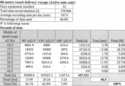
2.5.2 81 metre Vessel Data Records . 31

Contents

2.6 Data Analysis Methods . .

2.6.1 Data Manipulation .

2.6.2 Data Analysis . . . .

vii

34 34 35

3 Prediction of Vessel Response 38

3.1 Review of Alternative Methods Available 38

3.2 Basis of High Speed Strip Theory Method 40

3.2.1 Synopsis of the Green Function Method 41

3.3 The High Speed Strip Theory Program BESTSEA 44

3.3.1 Code Overview . . . 45

3.4 Modelling of Motion Control Surfaces 46

3.4.1 T-foil Force Model . . . 47

3.4.2 T-foil Force . . . 50

3.4.3 Transom Tab Force Model . 51

3.4.4 Transom Tab Force . . . 52

3.4.5 Application of Control Surface Force in Numerical Model 53

3.4.6 Force Capacity of Motion Control Surfaces . . . 53

3.4.7 Motion Control Method . . . 59

3.4.8 Deflection Velocity and Acceleration Restriction . . . . 77

3.4.9 Application of Motion Control with Transfer Functions 77

3.5 Development of Operating Interface Programs. 78

3.5.1 Motion Analysis . . . 79

3.5.2 Motion Derivation about the LCG . . . 80

3.5.3 Position of Minimum Motion in Regular Head Sea Waves 81

4 Full-Scale Experimental Results 84

4.1 Introduction. . . 84

4.2 Overview of Data Records . . . 84

4.3 Encountered Sea Conditions . . 89

4.3.1 Wave Height and Period . 89

4.3.2 Derived Wave Spectra . . 99

4.4 Vertical Accelerations . . . 107

4.4.1 Variation of Relative Acceleration with Longitudinal Position on

Vessel . . . 107

4.4.2 Variation of Relative Acceleration with Wave Height 111

4.4.3 Variation of Relative Acceleration with Wave Period 117

4.4.4 Measured Acceleration Spectra . . . 123

4.5 Measured Transfer Functions . . . 128

4.5.1 Measurements with Tabs Only on Delivery Voyages (81m and

86m vessels) . . . 128

4.5.2 Measurements with Tabs and T-foils for Operational Service (81m

and 86m vessels) 129

4.6 Summary . . . 131

5 Predicted Motion Results

5.1 Introduction . . . . 5.2 Selection of Speed and Loading Conditions . . . . 5.3 Modelling of Sea Conditions and Motion Control System .

5.3.1 Wave Period Selection . . . . 5.3.2 Wave Height Selection and Spectrum . . . .

5.3.3 Control Gain Settings with Active Controls

Contents viii

5.4 Effect of Speed on Transfer Functions . . . 147

5.4.1 With Fixed Motion Control Surfaces 150

5.4.2 With Active Transom Tabs Only . . 150

5.4.3 With Active Transom Tabs and Fixed T-foils 155

5.4.4 With Active T-foils Only . . . 155

5.4.5 With Active Transom Tabs and T-foils. . . 160

5.4.6 Comparison of the Effect of Control Modes 160

5.5 Vertical Accelerations . . . 164

5.5.1 Effect of Position on Vessel on Vertical Acceleration Spectra. 164

5.5.2 Effect of Speed on Average Acceleration Spectra . . . 169

5.5.3 Effect of Speed on Acceleration Relative to Wave Height . . . 174

5.5.4 Effect of Wave Period on Accelerations . . . 178

5.5.5 Effect of Position and Controls on Acceleration Relative to Wave

Height . . . 182 5.6 Effect of Regular Wave Height on Transfer Functions and Accelerations 184 5.7 Effect of MCS Target Wave Height on Acceleration Relative to Wave

Height . . . 192

5.8 Effect of Vessel Acceleration on Human Tolerance. 195

5.8.1 Motion Sickness Incidence . 195

5.9 Summary . . . 195

6 Comparison of computed and measured responses 199

6.1 Introduction . . . 199

6.2 Comparison of Transfer Functions . . . 199

6.2.1 Delivery Voyage Transfer Function Comparison 200

6.2.2 Service Operations Transfer Function Comparison 201

6.2.3 Effect of Wave Height on Transfer Functions with a More Recent

Prediction Program . . . 202

6.3 Comparison of Accelerations Relative to Wave Height . . . 209

6.3.1 Variation of Relative Acceleration with Wave Period 209

6.3.2 Variation of Acceleration with Longitudinal Position 209

6.4 Summary . . . 210

7 Discussion and Conclusions 214

7.1 Introduction . . . 214

7.2 Overall Conduct of the Sea Trials Program 214

7.3 Computational Investigation of Response . 216

7.4 Comparison of Measured and Computed Motions 217

7.5 Specific Outcomes of the Investigation . 219

7.6 Implications of Research . . . 221

7.7 Other Matters for Future Investigation . 221

A Hull particulars

A.1 81 metre Vessel (Hull 038) A.2 86 metre Vessel (Hull 042) .

B Experimental Instrumentation and Data

B.l Instrumentation on the 81 metre Vessel (Hull 038) B.1.1 TSK Wave Meter . . . . B.1.2 Analog to Digital Conversion Module B.1.3 GPS Connection . . . .

235 235 . 240

Contents

B.1.4 Motion Instrumentation Output . . . . B.1.5 Data Output . . . . B.2 Instrumentation on the 86 metre Vessel (Hull 042)

B.2.1 Motion Instrumentation . . . . B.2.2 Ship Electrical Junction Boxes B.2.3 Data Output . . . .

C Bestsea Hull Geometry Definition

D Labview program listing

E The Bretschneider Wave Spectrum

F Motion Analysis

F .1 Motion Sickness Incidence . . . . F.2 1/3 Octave Analysis of Acceleration Response .

ix

249 249 252 252 253 253

255

256

260

List of Figures

1.1 Lift reduction factor with depth/chord ratio. 6

2.1 81 metre (Incat Hull 038) - first experimental measurements . 17

2.2 86 metre (Incat Hull 042) - second experimental measurements 17

2.3 Minimum measurable wave length by a sea surface transducer. 20

2.4 Nomenclature and geometry used for the determination of the primary wave dirction. . . 22 2.5 Sign of roll and pitch angles for various angles of downward deck slope. 23

2.6 Primary wave direction predicted at 180°. 27

2. 7 Primary wave direction predicted at 225°. 28

2.8 Primary wave direction predicted at 90°. . 29

3.1 Diagram showing the variables applied in the lifting surface computation. 48 3.2 Steady state roll and pitch angle due to the maximum deflection force

of the motion control surfaces for the 81 and 86 metre vessels. . . 55 3.3 86 metre vessel response at forward speed in heave and pitch to sinusoidal

transom tab excitation in calm water (no T-foil). . . 56 3.4 86 metre vessel response at forward speed in heave and pitch to sinusoidal

T-foil flap excitation in calm water (no transom tab). . . 57 3.5 86 metre vessel response at forward speed in heave and pitch to sinusoidal

transom tab excitation with a fixed T-foil in calm water. . . 58 3.6 Variation in heave and pitch transfer functions between 1 and 2 iterations

of the gain finding routine (86m vessel, 32.5kn, active tab only, Loading condition: Service-Full departure) . . . 68 3.7 Variation in heave and pitch transfer functions (86m vessel, 32.5kn) for

active tab and T-foil configuration when gains are determined for indi-vidual surfaces or combined. . . 69 3.8 Gain optimisation example for single control surface. . . 74 3.9 Gain optimisation example for multiple control surfaces. . . 75 3.10 Optimum control surface phase (hence gains) for various configurations

and speeds. . . 76 3 .11 Variation in position of minimum vertical motion with encounter frequency. 83

4.1 Measured RMS wave height verse wave period of each data record. . . . 89 4.2 81 metre vessel measured RMS wave height verses average wave period

(T1 ) (12.5 to 42.5kn). . . 93 4.3 86 metre vessel measured RMS wave height verses average wave period

(T_{1 )} (12.5 to 22.5kn). . . 96 4.4 86 metre vessel measured RMS wave height verses average wave period

List of Figures _xi

4.5 86 metre vessel measured RMS wave height verses average wave period

(T1)

4.6 Measured wave spectra (81m vessel, tabs only). . . 103

4.7 Measured wave spectra (81m vessel, tabs and T-foils). 104

4.8 Measured wave spectra (86m vessel, tabs only). . . 105

4.9 Measured wave spectra (86m vessel, tabs and T-foils). 106

4.10 Measured acceleration verses hull position (81m and 86m vessels, 12.5 to 22.5kn) . . . 108 4.11 Measured acceleration verses hull position (81m and 86m vessels, 27.5

to 37.5kn). . . . 109 4.12 Measured acceleration verses hull position (81m and 86m vessels, 42.5kn).110 4.13 Measured LCG acceleration verses wave height (81m vessel, 12.5 to 42.5kn).113 4.14 Measured LCG acceleration verses wave height (86m vessel, 12.5 to 22.5kn) .114 4.15 Measured LCG acceleration verses wave height (86m vessel, 27.5 to 37.5kn).115 4.16 Measured LCG acceleration verses wave height (86m vessel, 42.5kn) . . . 116 4.17 Measured LCG acceleration verses average wave period

(T1)

12.5 to 42.5kn). . . 119 4.18 Measured LCG acceleration verses average wave period (T1 ) (86m vessel,

12.5 to 22.5kn). . . 120 4.19 Measured LCG acceleration verses average wave period (T1 ) (86m vessel,

27.5 to 37.5kn). . . 121 4.20 Measured LCG acceleration verses average wave period

(T1)

42.5kn). . . 122 4.21 Measured LCG acceleration response spectra (81m vessel, active tabs

only). . . 124 4.22 Measured LCG acceleration response spectra (81m vessel, active tabs

and T-foils). . . 125 4.23 Measured LCG acceleration response spectra (86m vessel, active tabs

only). . . 126 4.24 Measured LCG acceleration response spectra (86m vessel, active tabs

and T-foils). . . 127 4.25 Measured heave displacement transfer functions (81 and 86m vessels,

active tabs only) . . . 133 4.26 Measured roll displacement transfer functions (81and86m vessels, active

tabs only) . . . .- . . . 134 4.27 Measured pitch displacement transfer functions (81 and 86m vessels,

active tabs only) . . . 135 4.28 Measured heave displacement transfer functions (81 and 86m vessels,

active tabs and T-foils) . . . 136 4.29 Measured roll displacement transfer functions (81 and 86m vessels, active

tabs and T-foils) . . . 137 4.30 Measured pitch displacement transfer functions (81 and 86m vessels,

active tabs and T-foils) . . . 138

5.1 Transfer functions at various loading conditions (81m vessel, no control surfaces) in (a) heave and (b) pitch at 32.5kn. . . 142 5.2 Transfer functions at various loading conditions (86m vessel, no control

surfaces) in (a) heave a'nd (b) pitch at 32.5kn. . . 143 5.3 Bretschneider wave spectrum and corresponding head sea wave encounter

spectra as used in computations (Hs = 2.5m,

T1

List of Figures xii

5.5 Predicted pitch transfer functions (86m vessel, no control surfaces) . 149

5.6 PrediCted heave transfer functions (86m vessel, fixed tab and T-foil) 151

5.7 Predicted pitch transfer functions (86m vessel, fixed tab and T-foil) . 152 5.8 Predicted heave transfer functions (86m vessel, active tab only) . . . 153 5.9 Predicted pitch transfer functions (86m vessel, active tab only) . . . 154 5.10 Predicted heave transfer functions (86m vessel, active tab, fixed T-foil) . 156 5.11 Predicted pitch transfer functions (86m vessel, active tab, fixed T-foil) 157 5.12 Predicted heave transfer functions (86m vessel, active T-foil only) . . . 158 5.13 Predicted pitch transfer functions (86m vessel, active T-foil only) . . . 159 5.14 Predicted heave transfer functions (86m vessel, active tab and T-foil) . 162 5.15 Predicted pitch transfer functions (86m vessel, active tab and T-foil) . 163 5.16 Predicted acceleration response spectral density (86m vessel, 12.5kn) at

.(1) aft perpendicular (AP), (2) longitudinal centre of gravity (LCG), (3) forward perpendicular (FP) . . . 165 5.17 Predicted acceleration response spectral density (86m vessel, 22.5kn) at ·

(1) aft perpendicular (AP), (2) longitudinal centre of gravity (LCG), (3) forward perpendicular (FP) . . . 166 5.18 Predicted acceleration response spectral density (86m vessel, 32.5kn) at

(1) aft perpendicular (AP), (2) longitudinal centre of gravity (LCG), (3) forward perpendicular (FP) . . . 167 5.19 Predicted acceleration response spectral density (86m vessel, 42.5kn) at

(1) aft perpendicular (AP), (2) longitudinal centre of gravity (LCG), (3) forward perpendicular (FP) . . . 168 5.20 Predicted acceleration response spectral density (86m vessel, 12.5 knots,

average between 'positions on vessel) . . . 170 5.21 Predicted acceleration response spectral density (86m vessel, 22.5 knots,

average between positions on vessel) . . . 171 5.22 Predicted acceleration· response spectral density (86m vessel, 32.5 knots,

average between positions on vessel) . . . 172 5.23 Predicted acceleration response spectral density (86m vessel, 42.5 knots,

average between positions on vessel) . . . 173 5.24 Predicted vertical RMS acceleration per metre RMS wave height (86m

vessel) for various speeds at the aft perpendicular (AP), longitudinal centre of gravity (LCG) and forward perpendicular (FP) . . . 177 5.25 Predicted vertical acceleration (86m vessel, without control surfaces) at

(1) aftpeak (AP), (2) longitudinal centre of gravity (LCG), (3) forepeak (FP) . . . 18p 5.26 Predicted vertical acceleration (RMS) (86m vessel, fixed tab and T-foil)

at (1) aft perpendicular (AP), (2) longitudinal centre of gravity (LCG), (3) forward perpendicular (FP) . . . 181 5.27 Predicted vertical acceleration response distribution (86m vessel, 12.5

-42.5kn) . . . 183 5.28 Predicted heave and pitch transfer functions (86m vessel, 32.5kn,

with-out control surfaces). Comparison of computations at the regular wave heights of 0.5 and 2.5 metres (Loading condition: "Service-full depar-ture") . . . 187 5.29 Predicted heave and pitch transfer functions (86m vessel, 32.5kn).

List of Figures xiii

5.30 Predicted heave and pitch transfer functions (86m vessel, 32.5kn, various configurations) comparing computations at 0.5 and 2.5 metre regular wave height (Loading condition: "Service-full departure") . . . 189 5.31 Predicted acceleration response spectra (86m vessel, 32.5kn) for

compu-tations at 0.5 and 2.5 metre regular wave heights. . . 190 5.32 Predicted vertical acceleration (86m vessel, 32.5kn) for computations at

0.5 and 2.5 metre regular wave heights. . . 191 5.33 Predicted change in RMS acceleration (86m vessel, 32.5kn, "Service-Full

departure" loading condition) due to variation in the targetted regular wave height of control surface maximum deflection. . . 194 5.34 86 metre vessel predicted motion sickness incidence (MSI) over 2-hours

exposure duration . . . 198

6.1 Transfer function comparison in (a) heave and (b) pitch (86m vessel, 12.5kn, active tabs only) . . . 204 6.2 Transfer function comparison in (a) heave and (b) pitch (86m vessel,

32.5kn, active tabs only) . . . 205 6.3 Transfer function comparison in (a) heave and (b) pitch (86m vessel,

12.5kn, active tabs and T-foils) . . . 206 6.4 Transfer function comparison in (a) heave and (b) pitch (86m vessel,

32.5kn, active tabs and T-foils) . . . 207 6.5 Transfer functions in (a) Heave and (b) Pitch using BEAMSEA with

computations at various wave heights (86m vessel, 37.5kn, Hull loading condition not available) . . . 208

6.6 Comparison bet~een computed and measured acceleration per unit wave

height (RMS) at LCG in head seas for (a) active tabs and (b) Active tabs and T-foils (86 m.etre vessel) . . . 212 6.7 Comparison of predicted and measured distribution of acceleration per

unit wave height (RMS) in head seas for (a) active tabs and (b) Active tabs and T-foils (86 metre vessel) . . . 213

A.l Full motion control configuration with transom tabs and forward mounted T-foils (81 metre vessel, Hull 038) .. : . . . 235 A.2 Full motion control configuration with transom tabs and forward mounted

T-foils (86 metre vessel, Hull 042) . . . 240

D.1 BESTSEA time domain computation input configuration program 256

D.2 BESTSEA time domain numerical computation post analysis program 257

D.3 Motion control system phase optimization plotting program for

extract-ing the minimum phase angle. . . 258

List of Tables

2.1 Correction to the downward deck slope result of equation 2.8 . . . 23

3.1 Relationship between various strip or strip-like theories and some 3D theories . . . 39 3.2 Previous motion solution used to estimate the variables of active motion

control configuration . . . 62 3.3 Motion control surface phase estimated prior to first iteration and actual

phase achieved after the first iteration with the corresponding heave and pitch gain values calculated for the two loading conditions considered (86m vessel, Regular wave height of computation was 0.5m) . . . 65 3.4 Motion control surface phase estimated prior to second iteration and

actual phase achieved after the second iteration with the corresponding heave and pitch gain values calculated for the two loading conditions considered (86m vessel, Regular wave height of computation was 0.5m) . 66 3.5 Motion control surface phase estimated prior to first iteration and actual

phase achieved after the first iteration with the corresponding heave and pitch gain values calculated for the one loading condition considered (86m vessel, Regular wave height of computation was 2.5m) . . . 66

4.1 Measurement record durations (81m vessel) at various speeds and ob-served wave heading sectors . . . 87 4.2 Measurement record durations (86m vessel) at various speeds and

ob-served wave heading sectors . . . 88 4.3 Overall measured averages of wave height, average wave period, and their

ratio . . . _. . . 90 4.4 Measured wave heights (RMS) and wave periods grouped according to

speed and observed wave direction sectors (81 and 86m vessels) . . . 94 4.5 Ratio of wave period to measured wave heights (RMS) grouped according

to speed and observed wave direction sectors (81 and 86m vessels) . . . 95 4.6 Measured bandwidth parameters and skewness . . . ._ . . . 101 4. 7 Measured wave heights (RMS) and vertical accelerations (RMS) grouped

according to speed and predicted wave direction (81 and 86m vessels) 112

4.8 Measured wave periods and vertical accelerations (RMS) grouped ac-cording to speed and predicted wave direction (81 and 86m vessels) . . . 118

5.1 Acceleration per metre wave height (RMS) (86m vessel, Regular wave height of control surface maximum deflection= 2.5m, Loading condition:

"Service-full departure") . . . 175 5.2 Acceleration per metre wave height (RMS) (86m vessel, Regular wave

List of Tables xv

5.3 Acceleration per metre wave height (RMS) (86m vessel, 32.5kn, Regular wave height of control surface maximum deflection= 1.25m) . . . 192 5.4 Acceleration per metre wave height (RMS) (86m vessel, 32.5kn, Regular

wave height of control surface maximum deflection = 1.56m . . . 193 5.5 Average MSI over length of vessel computed in head seas at two loading

conditions . . . 196

A.1 Principle hull particulars (81m vessel) for delivery loading conditions 236 A.2 Principle hull particulars (81m vessel) for in service 1003 load conditions 237 A.3 Principle hull particulars (81m vessel) for in service 503 load conditions 238 A.4 Radius of gyration values (81m vessel) for a range of delivery and in

service loading conditions . . . 239 A.5 Motion control surface positions and sizes (81m vessel) . . . 239 A.6 Principle hull particulars (86m vessel) for delivery loading conditions . . 241 A.7 Principle hull particulars (86m vessel) for in service 1003 load conditions 242 A.8 Principle hull particulars (86m vessel) for in service 503 load conditions 243 A.9 Radius of gyration values (86m vessel) for a range of delivery and in

service loading conditions . . . 244

A.10 Motion control surface positions and sizes (86m vessel) 244

B.l Calibration values for wave meter . . . 248

B.2 Motions calibration (81m vessel) . . . 249

B.3 Channel configuration and header list for *.car files (81m vessel) 250

B.4 Instrumentation positions, channel configuration and header list for *.car files (81m vessel) . . . 251 B.5 Motions channel calibrations (86m vessel) . . . 252 B.6 Instrumentation positions, channel configuration and header list for *.car

files (86m vessel) . . . 254

Nomenclature

(a) Roman Symbols

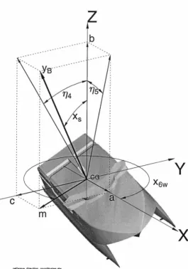
a Vector projection variable for wave direction determination

Ai Plan area of ith lifting surface

c

b Vector projection variable for wave direction determination

B Hull beam [m]

c Vector projection variable for wave direction determination

Ct Lift coefficient

Ctoo Lift coefficient without free surface effects

Cm Moment coefficient at quarter chord point

fs Data sampling frequency [Hz]

Fn Froude number

FL Lift force of ride control surface [N]

Ffwd Component of lifting surface force transferred to the forward adjacent section Faft Component of lifting surface force transferred to the aft adjacent section

g Gravitational acceleration constant = 9.81m/ s2

h Depth below mean free surface [m]

H 1 Significant wave height [m]

3

Hs Significant wave height by definition= 4.y'mO [m]

Hi Transfer function of the ith degree of freedom

Hw Height of regular waves [m]

k Wave number ( = 2{)

k44 Roll mass radius of gyration [m]

k55 Pitch mass radius of gyration [m]

k66 Yaw mass radius of gyration [m]

k46 Roll-yaw mass radius of gyration = k64 [m]

Kr,₃i Velocity based heave gain for the ith control surface

Kr,₅i Velocity based pitch gain for the ith control surface

L Length parameter (typically equivalent to waterline length or length between perpendiculars) [m]

Lpp Length between perpendiculars [m]

Lwl Length of waterline [m]

m Vector projection variable for wave direction determination

mo Zeroth moment of reponse or wave spectrum

m1 First moment of reponse or wave spectrum

m2 Second moment of reponse or wave spectrum

mk kth moment of reponse or wave spectrum

n Number of data samples

Nomenclature xv ii

Ni

N2 Po Pv q 83

s,(w) s,(we)

t

T T1 T2 u

u

Vo

w

Xs x.;,3(+)

Xi/3(-) Xa,

z

factor for calculating the appropriate number of time steps factor for calculating the appropriate number of time steps Total static pressure (pa+ pgh) [Pa]

Fluid vapour pressure [Pa] Dynamic pressure (0.5pV₀2 )

Response spectrum of the ith degree of freedom Wave spectrum ordinate

Wave encounter spectrum ordinate Time [s]

Hull draft [m]

Wave average period (or T)

Wave zero crossing period (or Tz)

horizontal wave particle velocity in time and space due to a regular long crested wave [m/s]

Constant vessel forward speed [m/ s2] Fluid free stream velocity (=U) [m/s2]

vertical wave particle velocity in time and space due to a regular long crested wave [m/s]

x axis of vessel coordinates (from LCG to bow)

longitudinal distance between the hull centre of gravity and the centre of control surface force application

Deck slope direction angle [radians or degrees]

Longitudinal distance from lifting surface position to the aft adjacent section Longitudinal distance from lifting surface position to the forward adjacent sec-tion

Deck slope magnitude [radians or degrees] Primary wave direction [deg or rad] Wave encounter direction [deg or rad]

Variable for calculating gains of ith control surface for local acceleration feed-back control

Variable of gains finding routine for ith surface deflection control

Variable for calculating position of minimum vertical motion

Variable for calculating gains of ith control surface for local velocity feedback control

y axis of vessel coordinates (from LCG to port)

Variable for calculating gains of ith control surface for local acceleration feed-back control

Variable of gains finding routine for ith surface deflection control Variable for calculating position of minimum vertical motion

Variable for calculating gains of ith control surface for local velocity feedback control

z axis of vessel coordinates (from LCG vertically upwards)

Nomenclature _{xv iii}

(b) Greek Symbols

a Incident angle of the free stream velocity on the main body of the lifting surface

ao

aw Incident angle created by the presence of waves ignoring the presence of hull

f3

Di Flap angle of ith control surface proportional to heave and pitch [rad]

Di Flap angle amplitude of ith control surface [rad]

of

ox

€3 Heave phase [radians]

€5 Pitch phase [radians]

€3v Heave velocity phase [radians]

csv Pitch velocity phase [radians]

€3a Heave acceleration phase [radians]

csa Pitch acceleration phase [radians]

ry₃ Heave displacement in time [m]

ry3! Heave response to T-foil sinudoidal flap oscillation [m]

ry₃t Heave response to transom tab sinudoidal oscillation [m]

ry_3tf Heave response to transom tab sinudoidal oscillation, T-foil fixed [m]

ry₄ Roll displacement in time [radians]

ry₅ Pitch displacement in time [radians]

rJsf Pitch response to T-foil sinudoidal flap oscillation [radians]

'f"/st Pitch response to transom tab sinudoidal oscillation [radians]

rJstf Pitch r~sponse to transom tab sinudoidal oscillation, T-foil fixed [radians]

ry₆ Yaw displacement in time [radians]

rJBw Direction of downward deck slope in time [radians]

77₃ Heave displacement amplitude [m]

7]5 Pitch displacement amplitude [rad]

i]₃ Heave velocity in time [m]

i]₅ Pitch velocity in time [rad]

7;₃ Heave acceleration in time [m]

7;₅ Pitch acceleration in time [rad]

()h Angle of free stream flow due to heave velocity and forward speed

B-p Angle of free stream flow due to pitch velocity and forward speed

A. Wave length [m]

µ Wave direction or primary wave direction [rad or deg]

µ,

µe Wave encounter direction [rad or deg]

( Free surface displacement from still water level [m]

( Wave amplitude [m]

p Sea water density= 1025 [kg/m3]

(}" Cavitation number

(=(po -

<P Motion control surface optimum phase at selected regular wave frequency [ra-dians]

<Pv Motion control surface phase at selected regular wave frequency (based on local velocity feedback) [radians]

<Pa Motion control surface phase at selected regular wave frequency (based on local acceleration feedback) [radians]

Nomenclature

e

w Wave frequency

[rad/

We Wave encounter (also flap oscillation) frequency

[rad/

w* Non-dimensional wave frequency=

w~

w:

We~

(c) Subscripts

1 Surge

2 Sway

3 Heave

4 Roll

5 Pitch

6 Yaw

(d) Acronyms

AP Aft perpendicular

F FT Fast fourier transform

FIR Finite impulse response

F P Forward perpendicular

GPS Global positioning system

IN A Institution of Naval Architects

ITTC International Towing Tank Conference

MCS Motion control system or motion control surface

MSI Motion sickness incidence

RINA Royal Institution of Naval Architects

SN AME Society of Naval Architects and Marine Engineers

UCL University College London

UTAS University of Tasmania

Chapter

1

Introduction

1.1

Development of High Speed Vessels and Emergence

of Motion Problems

High-$peed vessels have been operating for many decades and in development since the advent of the steam reciprocating engine in the early nineteenth century but high Froude number hull forms are of more recent design. With the ability to move directly into the wind also came the necessity to move directly into the waves, which increased the motions, loads and slamming type phenomenon (see Lewis (1988a)).

During the nineteenth century an 83ft vessel built in 1873 achieved 21 knots whilst a 147ft torpedo boat built in 1887 reached 26 knots. Speeds over 30 knots first appeared in 1896 with a 200ft torpedo boat called the Turbinia, a lOOft craft of 43-ton displacement, which achieved approximately 32 knots (see Dorey (1990)). In comparison, hydrofoils developed from 1897 to 1905 achieved speeds up to 50 knots in sheltered waters (see Coggeshall (1985)).

Navigation between continents remained the domain of slower sailing ships up un-til 1819 when the paddle steamer MV Savannah crossed the North Atlantic from the Savannah River to Liverpool in 27 days. From that time, passenger numbers began to increase as their reliability improved. When the steam turbine and multiple propellers replaced the steam reciprocating engine and paddle wheel, cruising speeds increased from 9 knots in 1838 with the Great Western to 29 knots in 1936 with the liners Nor-mandy and Queen Mary where they remained for the next few decades. Most of the existing liners had excellent seakeeping characteristics because of their length, large displacement and low metacentric height, a combination of hull parameters that are impossible to duplicate on smaller vessels (see Lloyd (1989)). At their high cruising speeds, these vessels were able to maintain acceptable seakeeping standards as their length based Froude numbers generally remained low, in a range below 0.3 (see Oth-fors and Ljungstrom (2003)). Maintaining acceptable roll motions was achieved with the provision of bilge keels and active roll damping mechanisms such as the roll fin introduced in 1890 (see Saul (1946)) or the gyroscopic roll stabilizer (see Scarborough (1958)), which was effective at reducing roll right down to zero forward speed.

With the advent of airline travel between continents, long distant travel by ship decreased and the liner was eventually replaced by the slower more economic cruise ship designed for the leisure market and generally slow short distance voyages.

Achieving higher speeds with displacement hull forms, required compact

1.1 Development of High Speed Vessels and Emergence of Motion Problems 2

1980s (see Hercus (1988)) made not only higher speeds possible but also higher Froude numbers. Compared with the traditional liner, cruise ship or conventional passenger ferry, these vessels were much shorter in length, had a shallow draft and in favourable wave conditions could achieve speeds of over 40 knots. As these designs matured, ap-proval was obtained for these vessels to operate in open water routes but the limited ability of the lighter structural design to withstand the loadings of larger wave heights, which were a high probability in open waters, meant that restrictions had to be im-posed. These included limiting the operational wave height and the provision that the route allowed the vessel to seek a sheltered harbour in the case of adverse wave condi-tions within a certain amount of time. Restricted wave height operacondi-tions also existed because the adopted novel evacuation systems required as part of their effective oper-ation, a relatively quick transition of personnel to the life rafts tethered along side in the event of a major fire outbreak or catastrophic structural failure due to for example, collision or grounding.

Shortly after the recruitment of high Froude number passenger vessels into service, large resonant heave motions were reported that caused severe discomfort and even

~Ihesis to a large proportion of the passenger population. This problem improved with the installation of motion control devices (see Hercus et al. (1991) and Adams (1996)), which were an existing technology but still in development for this type of application. Despite the improvement these devices made, it was common for the vessel's speed to be reduced in combination with a course change in the event of adverse wave conditions with the expectation this would improve passenger comfort and reduce the severity of wave impacts ~n the hull (see Dogliani and Bondini (1999)). Under the circumstances where a reduction in speed was sought, the high Froude number, operationally limited vessel would often find that its cruising speed would end up below 28 knots and thus no better than the cruising speed of the modern unrestricted steel Ro-Ro mono-hull ferries. Wave-induced motions and structural loads on these vessels therefore remain an important consideration if their operational limitations are to be improved.

Maintenance and versatility of recent motion control systems have improved to the point where hydraulic actuators are controlled from computer software through a digital network, but their force capability essentially remains a device size issue that must be considered in relation to the magnitude of wave forces on the hull. Unfortunately, the sizing of a motion control device is often a compromise with other hull design constraints such as hydrodynamic resistance and structural weight.

1.2 Vessel Motion in Waves ₃

enormously to that outcome.

For many, the complexity of a seakeeping analysis and the difficulty of extracting information that can make a useful contribution to the design process remains the largest obstacle for seakeeping prediction methods or model tests to be fully utilized (see Hearn (1991)). This problem is set to improve as some consensus and accuracy of numerical prediction methods improves and the presentation of useful results to the designer are standardized.

The prediction of motions and loads are some of the most heavily regulated and time consuming areas in ship design and these regulations are increasing as practical tools become more available. Higher hull speeds have increased the complexity of hull motions and loads so the scope and dimension of some long-standing problems in seakeeping remain. In particular, the magnitude of response at resonant frequencies is much more pronounced and coupling between degrees of freedom is more important, particularly for high Froude number vessels.

Motion and load prediction methods have steadily improved since the introduction of strip theory by Korvin-Kroukovsky and Jacobs (1957), \yith validation predominantly coming from experimental model tests. Whilst these tests form an invaluable part of the verification process, the complete solution may not be immediately clear until verified with full-scale experiments, particularly as numerical prediction methods overcome their inherent shortcomings and improve both their accuracy and reliability.

Saunders (Second printing 1982) in 1960 stated, "In a seaway, the ship is moved involuntarily in all its six degrees of freedom, by forces over which man has as yet only a rather feeble and certainly an inadequate control. Until this control is achieved, he should at least know what motions may be expected under any given set of conditions. At the time of writing he knows relatively little."

Seakeeping is one of the most important aspects of ship design as it relates to the on-board comfort and enjoyment of personnel while at anchor, vessel integrity and safety while at sea or the feel-good impression and perception of being on board a safe and seaworthy vessel (see Gaillarde (2002)). Non-linear motions exhibited by the high speed light craft (see Zhao and Aarsnes (1995)) make full scale tests more important if prediction methods are to be improved whilst maintaining an adequate check on the reality of the problem.

1.2 Vessel Motion in Waves

1.2.1 Experimental Model Studies

Formal seakeeping studies that preceded present day thinking commenced with the pioneering work of William Froude and his son Robert Edmund in the 1860s shortly before their first tank work in 1871. The first tanks in Europe appeared shortly after, but experimental model scale investigation of ship motions in waves did not begin until the first installation of wave makers in model basins in 1887 in Great Britain, 1894 in the Soviet Union and 1916 in the United States. Full-scale experimental testing and observations occurred later on a more organized basis in the early 1900s.

1.2 Vessel Motion in Waves ₄

guarantees to b~ confirmed. This can occur through validated numerical predictions, but usually sea trials or a model-testing program is required for verification (see Dussert-Vidalet et al. (1995) provides an example of this for a Corsaire 11000 mono-hull). Other validations made through tank tests are too numerous to list but by way of example, Gong et al. (1994) conducted model-tests specifically to validate a 2D strip theory method on an 80 metre catamaran at Froude numbers up to 0.67. Hudson et al. (1995) conducted model tests on a displacement catamaran with various hull separations for comparison with three potential flow prediction methods that included a three dimensional panel source distributiop. and simple strip theory. In the results it was observed that in some cases an unexplained lower frequency of response in the measured heave and pitch resonance peaks occurred compared with the predicted solutions.

Wellicome et al. (1995) conducted some generic model tests on a "series 60" hull and produced transfer functions and phases in heave, roll and pitch providing researchers with a reference on this hull type for numerical comparisons.

1.2.2 Analytical Predictions

1.2 Vessel Motion in Waves 5

long computation time to obtain a solution that cannot not fully achieve validation by experiment, particularly at high Froude numbers.

1.2.2.1 Motion Control

For prediction codes to be useful to the designer, they must also have the capacity to deal with the non-linear effects introduced by a motion control system. Since the early 1990s as the high Froude number passenger vessel developed, such systems are considered a necessity (see Adams (1994), Adams (1996), Akers (1999)) to reduce the large heave excitations observed, to reduce fuel consumption through improved hull resistance in waves (see Burns (1990)) and to improve passenger comfort through reduced accelerations.

Any numerical ship motion prediction method can utilize motion control devices in the computation and numerous publications have reported such attempts in both the frequency and time domain. However, without a common method of control, appendage size and type, results will remain unique to a particular hull form and motion control appendage configuration.

Kvalsvold et al. (1999) investigated the operability of a high speed mono-hull fitted with a motion control system and experimented with a range of control coefficients to determine the operapility against a range of motion criteria. Improving the operability depended on the selection of devices combined with an appropriate selection of control coefficients.

Kang and Gong (1995) modelled the effect of motion,control fins on a catamaran with a time domain solution formulated to solve the wave exciting force with a 3D transient Green function (see Wehausen and Laitone (1960)). Using transient hydro-dynamic theory of Newman (1977), the force reduction and change in the force phase due to the sinusoidal change in fin angle of attack and sinusoidal wave particle veloc-ity were accounted for using the Wagner and Kussner functions respectively. The flap angle was limited to the assumed stall angle of 35 degrees at approximately 20 knots (Fn=0.548) vessel speed but did not address the possible effects of cavitation.

Ohtsubo and Kubota (1991) modelled a hydrofoil with a time domain strip theory that included a steady lift component, an unsteady component due to the orbital wave motion using gust theory, an unsteady component due to the ship motions and finally, the lift reduction due to the proximity of the free surface. The lift due to the proximity of the free surface was based on experimental results, which increased exponentially from approximately zero at the free surface to a maximum at some depth below five chord lengths. Their definition had the advantage that it accounted for the angle of attack of the foil at a given depth by decreasing the foil lift as the angle of attack1 increased. Wadlin and Christopher (1958) produced a theoretical derivation to account for foil depth effects but their formulation was much less influenced by the foil angle of attack. At moderate attack angles (say 6°), their formulation began to resemble th~t of Ohtsubo and Kubota (1991) where the lift reduction with depth occurred at approximately the same rate, but this quickly changed with only a few degrees change in foil angle of attack. Wadlin and Christopher (1958) also determined the lift generated by a planning surface, such as a foil as it rides over the free surface and changes from a submerged lifting device to a planning surface, which for shallow draft high Froude number hull forms is a distinct possibility. Fossen (1994, p 383) also accounted for a reduction in lift due to foil depth that changed linearly from a factor of 0.5 at the

1 _{Increased foil camber also had an effect but the foils discussed in this work are symmetrical, thus}

1.2 Vessel Motion in Waves 6

free surface to a factor of one at a depth equivalent to one chord. (see figure 1.1 for a comparison in the lift reduction factor at an angle of attack of 8 degrees) Theoretical and experimental work conducted by Lee et al. (1997) on fins mounted on a strut showed that the free surface influenced the foil lift for submergence depths less than three chord lengths.

1.1

1.0

~o.9 ~

.!!!

c:

~0.8

:::i

"C

l!! ;!: -'0.7

0.6

05

v

/

rj

v

I

~

-

-

~ ~

t.-e-

-v

0 Ohtsubo and Kubota (1991) 6. Fossen (1994)

0 Wadlin and Christopher (1958)

0 2 3 4 5 6 7 8 9 10

Foil depth/chord ratio

ref/ploLF01l-l1tt-reductlon-factor.gle

Figure 1.1: Lift reduction factor with depth/chord ratio. (foil angle of attack a= 8°, chord

==

Schellin and Rathje (1995) developed a 3D potential theory for predicting hull motions using pulsating sources and included the lift generated by cantilevered motion control fins. The lift calculation based at the fin centre of pressure included the influence of incident waves made up of the wave particle velocities, the translation and rotation due to the ship's motion and forward speed. Neglected are the effect of radiated and diffracted waves, down wash between fins, free surface influence and blockage of the other hull. Included is the body-fin interaction using the procedure given by Lee and Curphey (1977) (see also the original source Pitts et al. (1959)). This empirical formula considered the lift generated on the hull due to the cantilevered fin and the lift on the cantilevered fin due to the hull. The modelling in detail of further effects was considered to be a difficult task to accomplish satisfactorily. Each fin was located on the inboard side of the SWATH demi-hulls.

1.3 Development of Full-Scale Motion Measurements 7

1.3 Development of Full-Scale Motion Measurements

Full-scale measurements and the collection of data from ships at sea were a need that had existed for a long time before Kent (1924) (see also Kent (1927)) commenced some work by making six ocean voyages on three passenger liners. The observations reported the environmental conditions and the ship response to these conditions (see Korvin-Kroukovsky (1961, pp. 183-184)) generally using only the standard ship equipment. The only specialized equipment was for measuring roll and pitch angles with a flywheel type device and pen recorder. During this period, J. L. Kent presented only a small part of the collected material in numerous papers, which was related in no small part to the difficulty in post processing the information.

The measurement of heave, roll and pitch simultaneously over long time periods was possible after the development of the accelerometer and gyro-type sensor combined with a simultaneous pen recorder. Korvin-Kroukovsky (1961) noted that prior to 1955, no comparison of calculated and measured ship model motions had been made, despite the existence of full-scale measurements and mathematical methods. The first comparison

was conducted by Korvin-Kroukov~ky and Lewis (1955). Research methods improved

with the introduction of the portable computer, so large amounts of data could be collected over long periods and processed simultaneously or stored for later analysis.

The study of motion and loads potentially involves complex motion and vibration problems that can include any number of degrees of freedom. Experimentation at model scale remains the prime means of comparison as wave conditions can be prescribed and it can be the most efficient means to obtain a result. However, scale effects can often reduce the accuracy and reliability of the results when they are not fully understood so full-scale experimentation remains a valuable option in the numerical validation process.

1.3.1 Motion Measurement

Full-scale measurements have often been undertaken in conjunction with hull moni-toring programs in which data was recorded during routine vessel operations and in some cases over an extended period of time, such as those conducted by Vulovich et al. (1989), Beaumont and Robinson (1991), Brown et al. (1991), Witmer and Lewis

(1994), Witmer and Lewis (1995). and Cannon and Mutton (1997). In some instances

the measured data was not only stored for post-analysis, but was used to present the crew with real time hull motions, loads and wave conditions, thus providing an addi-tional resource that could contribute to the ship operations decision-making process. Dogliani arid Bondini (1999) made long term measurements on a high speed mono-hull whilst in operational service but had to rely on visual estimations and hind cast data to determine the dominant wave direction for each data record.

Stan-1.3 Development of Full-Scale Motion Measurements 8

dardisation, ISO 2631/3 (1985) and motion sickness incidence according to O'Hanlon and McCauley (1974) for a 52 metre catamaran fitted with a motion control system. Yum et al. (1995) conducted full-scale measurements on an actively controlled foil catamaran and made comparisons with a simple strip theory and 3D panel method by deriving root mean square responses for comparisons of heave, roll and pitch. Boulton (1999) used full-scale measurement data from a new vessel to verify its seakeeping and for comparison with previous vessels. Rantanen et al. (1995) used full-scale measure-ments to confirm the seakeeping performance of a new vessel and to evaluate numerical predictions and model tests, as did Schellin and Papanikolaou (1991) for a SWATH hull form in which comparative transfer functions were presented. Wang et al. (1999) used full-scale measurements on a mono-hull to evaluate both linear and non-linear nu-merical methods. Thompson (1979) conducted extensive full-scale measurements on an Attack Class ;patrol Boat and was able to derive response spectra and transfer functions for roll and pitch using a wave rider buoy and analogue instrumentation techniques. Haywood and Duncan (1997) used full-scale measurements on high-speed ferries to tune a motion control system using a system identification techniques. Aksu et al. (2002) performed full-scale trials on a twin hull 86 metre vessel, which was a similar type to the 86 metre vessel used for the present study. They conducted motion measurements at various wave headings and speeds for comparison with a numerical three-dimensional panel method. Finally, as part of the program of extensive ship monitoring and data recording conducted by Witmer and Lewis (1994) and Witmer and Lewis (1995), it was important to provide feedback of the measurements to the crew by means of a display monitor mounted on the bridge during the monitoring period so they could make appropriate decisions and take action to maintain the ship operation within the defined loading limits. This required almost real time data post processing and data storage.

1.3.2 Wave Measurement

Wave measurement instruments broadly fall into two categories that include point measurement or spatial averaging devices. Wave rider buoys contairnng instrumentation or pressure sensors generally fall under the former description and can provide either omni- or uni-directional wave statistics (see Clauss et al. (1999)). Satellites fall into the description of spatial averaging devices that require calibration with a wave rider buoy but are generally unsuitable for providing local wave statistics in real time for a vessel at sea.

The Darbyshire wave spectrum was developed with a ship borne wave recorder (see Tucker (1952)) that consisted of a pressure gauge mounted on the hull approximately lOft below the free surface on both the port and starboard side. Combined with each gauge was an integrating accelerometer that recorded the stationary ship's heave motion over 7 to 10 minutes (see also Tucker (1956), Tucker (1991)).

Cartwright (1956) tried to measure the directional distribution of waves in the open sea using a ship mounted wave recorder that could be analysed to obtain a scalar spectrum. By steering the ship around a regular dodecagonal circuit (12 sided) at 7 knots, the directional sensitivity was determined through calculating the "Doppler shift". Theoretically it was possible to determine the directional spectrum from this procedure but the variability in the spectral estimates were too great due to the short sample duration of 12 minutes to make the evaluation practical (see Korvin-Kroukovsky (1961)).

1.3 Development of Full-Scale Motion Measurements ₉

experimentally. In other work Barber (1954) used a row of detectors mounted on wharf piles, each consisting of a pair of parallel vertical copper strips partly immersed in the water, but this was not demonstrated for use as a ship borne system. Similarly, Dipper (1987) evaluated various methods to accurately estimate the directional components of ocean and basin waves to assist with requirements for manoeuvring and seakeeping tests. He went on to examine a method to estimate the directional wave spectra through an application of the Maximum Likelihood Method (MLM). This method was capable of such estimates provided the spacing of the fixed wave probe arrays were tuned spatially with respect to the frequency content of the waves for which a directional spectrum is to be estimated. He had better success with closely spaced wire capacitance transducers than a broadly spaced ultrasonic transducers. This problem was related to the poor tuning of the sonic transducers to the analysed wave conditions. The procedure was well equipped to determine the directional wave spectra for presentation and analysis at both full and model scale, but the method implies that the transducer mounting must be fixed in space.

Investigations using full-scale ship motions alone to estimate the wave spectra were undertaken by Marks (1967). Hua and Palmquist (1995) determined the wave spectra

from hull response measurements, which they called the variation method. These proved

to be successful in bow waves but following wave directions gave unsatisfactory results. Bachman et al. (1987) investigated the use of a surface following wave buoy for application to full-scale measurement and analysis. They noted that there were differ-ences between the frequency of ship encountered waves and buoy encountered waves, which could be increased if the buoy was free to move with a current moving in the opposite direction to the vessel. Furthermore, it could not be guaranteed that the wave data recorded would correspond to those encountered by the vessel as the trials course would often take the vessel some distance from the buoy location.

Recent developments make use of ultrasonic, laser, infrared or microwave trans-ducer (more details in sections 1.3.2.1 to 1.3.2.4 respectively) techniques for making uni-directional relative distance measurement from a vessel to the sea surface. More sophisticated radar systems are better described as a far field devices that provide directional wave spectra to a base of either wave or encounter frequency. These trans-ducers have the ability to scan the sea surface that surrounds the vessel, from which the statistical surface heights may be determined as a function of wave height and wave direction.

1.3.2.1 Ultrasonic Transducers

For particular applications the ultrasonic transducer makes a relatively low cost dis-tance ranging device. They can only operate at the speed of sound so their maximum sample rate is a function of the time taken for a sound pulse to be transmitted and received over the range being measured. These units are also subject to ambient temper-ature variations that can be allowed for with tempertemper-ature compensation. High sample rate is thus associated with short range measurement whilst long range measurement must suffer a reduction in sample rate. (section 2.2.1 discusses sample rate issues).

1.3 Development of Full-Scale Motion Measurements 10

1.3.2.2 Laser Transducers

Whilst laser units are expensive and their delicate construction make them prone to breakage, they can make excellent ranging devices for wave measurement (see Slotwinski et al. (1989)). Experience with these units showed that a return signal is possible whilst operating at low grazing angles 2 _{to the free surface. In principle, the laser units required} a relatively high number of returns in order to determine the range measurement with an acceptable order of accuracy. For example, over a range of 10 metres to achieve an accuracy of 0.1 metres the maximum sample rate is limited to 1 Hertz.

1.3.2.3 Infra.red Transducers

Infrared transducers have been used with success for wave height measurement on fixed platforms and was used with success for wave measurement from a moving vessel for deriving wave encounter spectra by Steinmann et al. (1999). They have a range of up to 50 metres and have been used primarily for fixed position wave height measurement.

1.3.2.4 Microwave Transducers

The microwave transducer has been used successfully in previous studies such as those by Yasuda et al. (1985) .and Rantanen et al. (1995) that produced a ship borne type microwave Doppler radar for full-scale measurements. The work of the former sub-sequently became the microwave unit of Tsurumi Seiki Co. Ltd. (TSK) (see TSK (2003)). Dipper (1997) attempted to measure the waves with a TSK ship borne radar, which on occasion was compared with a wave rider buoy by holding the vessel station-ary. Good agreement was obtained between the two measurement systems except at very low frequencies (approximately 0.06 Hz) where the TSK results appeared to be slightly attenuated. Steinmann et al. (1999) concluded from experiments with a TSK microwave radar and a Thorn infrared meter, that there was little difference between the two apart from erroneous low frequency results in the wave spectra of the TSK unit. Korvin-Kroukovsky (1961, pp. 67-68) suggested that such effects may be the result of d-c drift in the recording electronics where the wave record drifts away from the preset zero of the recorder. This is manifest in the spectrum as a spike at or near the zero frequency and corresponds to the apparent infinite wave period generated by the drift. This can be a particular problem for ship mounted wave sensors that move with the speed of the ship as there is difficulty in measuring low frequency components, partic-ularly if there are wave components travelling in the same direction as the vessel. This proposition contributes to the likelihood of not detecting any following wave patterns moving in the direction of vessel travel, which may exclude waves whose headings are aft of the beam from forming part of a seakeeping analysis when a fixed ship mounted sea surface sensor is used. Generally the linear drift is not a serious problem if the measurement application is planned with appropriate filters.

It was a similar TSK microwave transducer device that was installed on vessels for wave measurements in the present analysis.

1.3.3 Spectral Derivation

There are various accounts given on the analysis procedure adopted for full-scale anal-ysis. A general overview has been given by Bendat and Piersol (1980), Beauchamp and Yuen (1979) and more particular application to sea spectrum derivation by Korvin-Kroukovsky (1961).