Multi fidelity optimization via surrogate modelling

Multi-fidelity optimization via

surrogate modelling

BY ALEXANDER I. J. FORRESTER*, ANDRA´ S SO´ BESTER AND ANDY J. KEANE

Computational Engineering and Design Group, School of Engineering Sciences, University of Southampton, Southampton SO17 1BJ, UK

This paper demonstrates the application of correlated Gaussian process based approximations to optimization where multiple levels of analysis are available, using an extension to the geostatistical method of co-kriging. An exchange algorithm is used to choose which points of the search space to sample within each level of analysis. The derivation of the co-kriging equations is presented in an intuitive manner, along with a new variance estimator to account for varying degrees of computational ‘noise’ in the multiple levels of analysis. A multi-fidelity wing optimization is used to demonstrate the methodology.

Keywords: co-kriging; kriging; noise; subset selection; wing design

1. Introduction

Let f(x) denote an objective function that maps a vector x of length kto some scalar measure of merit. x is sought, such that f(x) is the maximum or minimum off(x). Suchoptimizationproblems (of which this is the simplest form) are encountered in most branches of science. Of interest to us in this paper is the class of optimization problems where f(x) is expensive to obtain or we know its value only at a limited number of x values. Thus, efficiency, in terms of the number ofxvalues that must be mapped to their objective function values before we get to within a reasonable distance ofx, is the key feature of the optimization algorithms considered.

While there is often no getting around the fact that a thorough search of a highly nonlinear, multi-dimensional flandscape will require sampling at a large number of sites, a useful shortcut is often employed. Based on a relatively small number of measurements, we can build a statistical approximation of the objective landscape, which, provided f is smooth and continuous and the measurements are reasonably uniformly spread, will be accurate enough to guide the search towards promising areas of the landscape.

If, at the same time, thissurrogate of the expensive function is very cheap to evaluate, we can be as thorough as we like in searching it. Thus, most of the computational effort will be concentrated on what looks likely to be the

Published online 2 October 2007

* Author for correspondence ([email protected]).

neighbourhood of the global optimum. An approximation technique that has received much attention in recent years is kriging1—we shall delve into the details of this later on, as our chosen multi-fidelity optimization technique is an extension of kriging. But what exactly do we mean by multi-fidelity optimization?

The objective function evaluation system may feature lower-fidelity, cheaper models (in addition to the main, high-fidelity calculation off). In most cases, the fast (but less trustworthy) and the slow (but more accurate) objective values can be obtained independently. Thus, we can learn more about the objective function by additionally measuring the cheap function(s) on a large number of x values. This process is usually referred to as multi-fidelity optimization.

The use of secondary, correlated quantities to improve the accuracy of the model of the primary objective is not a new concept. For example, Hevesiet al.

(1992)predict average annual precipitation values near a potential nuclear waste

disposal site using a sparse set of precipitation measurements from the region along with the correlated and more easily obtainable elevation map of the area.

Kennedy & O’Hagan (2000)approach the subject from the perspective of model

building using objectives resulting from computational simulations of varying fidelities and costs. This is also the context of the work presented here; additionally, we introduce a method of optimization using correlated models of different costs and fidelities. We focus on combining co-kriging (the multi-response extension to kriging alluded to earlier) with a Bayesian model update criterion designed to balance the exploration of the search space and the quick exploitation of promising basins of attraction on theflandscape. The criterion is based on a newly derived error estimate that reflects the presence of noise in the observed data.

After a brief overview of kriging in§2, we discuss co-kriging in§3, followed by considerations on how to create sampling plans for multiple levels of analyses (§4). We put these pieces together in §5, where we describe an optimization strategy designed for multi-fidelity inputs. An aircraft wing design problem is used to demonstrate and compare the co-kriging approach and other multi-level strategies in §6. Section 7 discusses the remaining issues related to the use of correlated surrogates and summarizes our conclusions.

2. Kriging

We will consider co-kriging as a natural extension to the popular method of kriging and hence begin with a very brief introduction to the kriging method in order to introduce concepts and notation that follow through to co-kriging. Equations are shown without derivations, which are very similar to those presented later for co-kriging; the reader may wish to consult Jones (2001) or

Forrester et al. (2006b) for more information on kriging.

As with all surrogate-based methods, to approximate a functionfwe start with a set of sample data—usually computed at a set of points in the domain of interest determined by a sampling plan (which will be discussed further in §4).

1_{Originally called krigeage by Matheron (1963) after D. G. Krige—a South African mining}

The kriging prediction of f is built from a mean base term, m^ (the circumflex denotes a maximum likelihood estimate, MLE) plus a stationary Gaussian process, Z(x), representing the local features of f around the n sample points, X_Zfxð1Þ;_.;xðnÞgT,x₂Rk. Z(x) has zero mean and covariance

cov½ZðxðnC1Þ

Þ;ZðxðiÞÞZs2jðiÞ; ð2:1Þ

where jðiÞ are correlations between a random variable Y(x) at the point to be predicted (x(nC1)

) and at the sample data points

jðiÞ_Zcorr½YðxðnC1Þ

Þ;YðxðiÞÞ_Zexp K Xk

jZ1

^

qjkx ðnC1Þ

j Kx

ðiÞ j k

^

pj

!

: ð2:2Þ

Thehyper-parameter, pj, can be thought of as determining the smoothness of the function approximation. In many situations, we can assume that there will not be any discontinuities and usepjZ2 rather than using an MLE. This means that the

basis function is infinitely differentiable through a sample point (when kxðnC1Þ_KxðiÞ_k

Z0) and that the function is in the same form as a Gaussian

distribution with variance 1=q^j.q^therefore can be thought of as determining how

quickly the function changes as x(nC1)

moves away from x(i), with high and low ^qj values indicating an active or inactive function along dimension j,

respectively. The kriging prediction is found as the value at x(nC1)

that, maximizes the likelihood, given the sample data and MLEs of the hyper-parameters, and is given by

^

yðxðnC1Þ_Þ

Zm^C Xn

iZ1

bðiÞjðiÞðxðnC1Þ_;xðiÞ_{Þ: ð2:3Þ}

The constantsbiare given by the column vectorbZJK1ðyK1m^Þ, whereJis an

n!n symmetric matrix of correlations between the sample data; y is a column vector of responses, fyðxð1ÞÞ;_.; yðxðnÞÞgT; 1 is an n!1 column vector of ones; and the MLE m^_Z1TJK1_y=1T_JK1_1.

3. Co-kriging

We now consider how to build an approximation of a function that is expensive to evaluate which is enhanced by data from cheaper analyses of the function. Combining multiple sets of data naturally leads to a complex notation and we will try to simplify this by limiting ourselves to two datasets:2the most accurate expensive data with valuesyeat pointsXeand the less accurate cheap dataycat points Xc (Xe3Xc).3 These data are concatenated to give the combined set of points

X_Z Xc

Xe !

Zðxðc1Þ;.;xðnc cÞ;xð 1Þ

e ;.;xðne eÞÞ T

:

2

Our methods can be extended to multiple code levels following the notation used byKennedy & O’Hagan (2000).

3_{We require partially collocated points in our estimation of a scaling parameter between the data.}

As with kriging, the value at a point inXis treated as if it were the realization of a Gaussian random variable. For co-kriging, we therefore have the random field

Y Z

YcðXcÞ

YeðXeÞ !

ZðYcðxðc1ÞÞ;.;Ycðxðnc cÞÞ;Yeðxðe1ÞÞ;.;Yeðxðne eÞÞÞT:

We follow the auto-regressive model of Kennedy & O’Hagan (2000), which assumes that cov YeðxðiÞÞ;YcðxÞjYcðxðiÞÞ

Z0,cxsxðiÞ. This means that no

more can be learnt about YeðxðiÞÞ from the cheaper code if the value of the expensive function atx(i)is known—a Markov property (i.e. we assume that the expensive simulation is correct and any inaccuracies lie wholly in the cheaper simulation). Gaussian processesZc($) andZe($) represent the local features of the cheap and expensive codes. Using the auto-regressive model, we are essentially approximating the expensive code as the cheap code multiplied by a scaling factor r plus a Gaussian process Zd($) that represents the difference between rZc($) and Ze($)

ZeðxÞZrZcðxÞCZ_dðxÞ: ð3:1Þ Whereas in kriging we have a covariance matrix covfYðXÞ;YðXÞg_Z s2JðX;XÞ, we now have a more complex covariance matrix constructed as follows:

covfYcðXcÞ;YcðXcÞg ZcovfZcðXcÞ;ZcðXcÞg

Zs2cJcðXc;XcÞ;

covfYeðXeÞ;YcðXcÞg ZcovfrZcðXcÞCZ_dðX_cÞ;Z_cðX_eÞg

Zrs2cJcðXc;XeÞ;

covfYeðXeÞ;YeðXeÞg ZcovfrZcðXeÞCZ_dðX_eÞ;rZ_cðX_eÞCZ_dðX_eÞg

Zr2covfZcðXeÞ;ZcðXeÞgCcovfZdðXeÞ;ZdðXeÞg

Zr2s2cJcðXe;XeÞCs2_dJ_dðX_e;X_eÞ:

The notation JcðXe;XcÞ, for example, denotes a matrix of correlations of the form jcbetween the data Xeand Xc. Our complete covariance matrix is thus

C_Z s

2

cJcðXc;XcÞ rs2cJcðXc;XeÞ

rs2cJcðXe;XcÞ r2s2cJcðXe;XeÞCs_d2J_dðX_e;X_eÞ !

: ð3:2Þ

The correlations are of the same form as equation (2.2), but there are two correlations, jc and jd, and we therefore have more hyper-parameters to estimate: qc; qd; pc; pd; and the scaling parameter r. Our cheap data are considered to be independent of the expensive data and we can find MLEs formc, s2c,qcand pcby maximizing the ln-likelihood (ignoring constant terms)

K

nc 2 lnðs

2 cÞK

1

2lnjdetðJcðXc;XcÞÞjK

ðycK1mcÞTJcðXc;XcÞK1ðycK1mcÞ 2s2

c

:

By setting the derivatives of equation (3.3) w.r.t.mcands2c to 0 and solving, we find MLEs of

^

mcZ1 T

JcðXc;XcÞ K1

yc=1 T

JcðXc;XcÞ K1

1 ð3:4Þ and

^

s2cZðycK1m^cÞ T

JcðXc;XcÞK 1

ðycK1m^cÞ=nc: ð3:5Þ Substituting equations (3.4) and (3.5) into (3.3) yields the concentrated ln-likelihood

K

nc 2 lnðs^

2 cÞK

1

2lnjdetðJcðXc;XcÞÞj ð3:6Þ andq^candp^c (if not set at2) are found by maximizing this equation.

To estimate the mean, variance, hyper-parameters and scaling parameter of the difference model (md, s2d,qd,pd and r), we first define

d_ZyeKry_cðX_eÞ; ð3:7Þ

where yc(Xe) are the values of yc at locations common to those of Xe (the Markov property implies that we need to consider only this data). If yc is not available at Xe, we may estimate r at little additional cost by using kriging estimates y^cðXeÞ, found from equation (2.3), using the already determined hyper-parameters q^c and p^c. The ln-likelihood ofd, given yc, is now

K

ne 2 lnðs

2 dÞK

1

2lnjdetðJdðXe;XeÞÞj

K

ðdK1m_dÞTJ_dðX_e;X_eÞK1ðdK1m_dÞ

2s2_d ; ð3:8Þ

yielding MLEs of

^

mdZ1 T

JdðXe;XeÞ K1

d=1TJdðXe;XeÞ K1

1

and

^

s2dZðdK1m^_dÞTJ_dðX_e;X_eÞK1ðdK1m^_dÞ=n_e; ð3:9Þ withq^d, p^d (again, if not set at 2) and r^found by maximizing

K

ne 2 lnðs^

2 dÞK

1

the time required to find MLEs can be reduced by using a constantqc,jand qd,j for all elements ofqcandqdto simplify the maximization, though this may affect the accuracy of the approximation.

With the hyper-parameters estimated, the co-kriging prediction of the expensive function is given by

^ yeðxðne

C1Þ

Þ_Zm^CcTCK1ðyK1m^Þ; ð3:11Þ where

c_Z r^s^

2

cjc Xc;xðnC1Þ

^

r2s^2cjc Xe;xðnC1Þ

Cs^2_dj_d X_e;xðnC1Þ

!

and m^Z1TCK1_y=1T_CK1_{1. The notation jc X}

e;xðnC1Þ

, for example, denotes a column vector of correlations of the form jcbetween the data Xeand the new point x(nC1)

. The derivation of equation (3.11) is given in appendix A. If we make a prediction at one of our expensive points, xðnC1Þ

ZxðiÞe and c is the

ncCith column of C, then cTCK1 is the ncCith unit vector and y^_eðx

ðiÞ

e ÞZ ^

mCy_ðncCiÞKm^Zy

ðiÞ

e . We see, therefore, that equation (3.11) is an interpolator of the expensive data. If we make a prediction at one of the cheap points, xðnC1Þ

ZxðiÞc ,cis not a column ofCand the predictor will in some sense regressyc unless it coincides with ye.

The estimated mean-squared error in the predictor is given as follows:

s2ðxÞZ^r2s^2cCs^2_dKcTCK1c: ð3:12Þ Again, a derivation is given in appendix A. Since the co-kriging model is an interpolator ofye, we expect the error to be zero at the expensive sample points. For xðneC1Þ

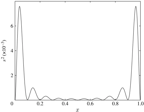
ZxðiÞe ,cTCK1is thencCith unit vector,cTCK1c_ZcðncCiÞ_Zr2_cs2_cCs2_d and hences2(x) is indeed 0. ForXc\Xe,s2(x)s0 unlessyeZyc(Xe). The error at these points is determined by the character ofYd. If the difference betweenrYc(Xe) and Ye(Xe) is simple (characterized by lowqd,jvalues), the error will be low, whereas a more complex difference (highqd,jvalues) will lead to high error estimates.

(a) One-variable demonstration

We will now look at how co-kriging behaves using an example of a simple one-variable function. Imagine that our expensive to compute data are calculated by the function feðxÞZð6xK2Þ

2

sinð12xK4Þ, x₂f0;1g, and a cheaper estimate of this data is given by fcðxÞZAfeCBðxK0:5ÞKC. We sample the design space extensively using the cheap function at XcZf0;0:1;0:2;0:3;0:4;0:5;0:6;0:7;0:8;0:9;1g, but run the expensive function only at four of these points, XeZf0;0:4;0:6;1g.

Figure 1 shows the functions fe and fc with AZ0.5, BZ10 and CZK5. A

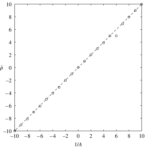
We have chosen the relationship between our low- and high-fidelity test functions in order to show how the hyper-parameters of the co-kriging model behave. The hyper-parameters pertaining to the cheap data,qcandpc, are affected only by this data and behave as described in§2. Moving on to the scaling parameter r, if our cheap model parameterA (the multiplying term linking the cheap and expensive functions) is varied such that 1=A₂fK10;10g, we obtain the values for

^

rshown infigure 3and see thatr^_x1=A. Similar trials show that the parametersB

andChave no effect onr; thus we see thatris purely a scaling parameter. Note that

^

ris only anindicatorof the scaling, since this value is estimated based on the data

0.2 0.4 0.6 0.8 1.0

0 2 4 6

2

(×10

–3)

Figure 2. Estimated error in the co-kriging prediction infigure 1. The simple relationship between the data results in low error estimates atXcas well asXe.

0 0.2 0.4 0.6 0.8 1.0

–10 –5 0 5 10 15 20

kriging through co-kriging

available. For the data in figure 1,r^_Z1:87 (close to the true value of 2), but for small samples ofyethe MLE may be misleading. The slight deviations of the data in

figure 3fromr^Z1=A(shown as a dashed line), the most significant of which is at

1/AZ6, are where our GA search has not found the true MLE.

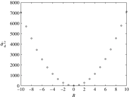
Recall that dZyeKrycðXeÞ (equation (3.7)) and hence, with r^zye=yc, d represents the difference in trends between the cheap and the expensive data. Thus, for our one-variable example, whenB,CZ0,md^ ;s^2d/0 for all values ofA, ifr^is estimated accurately.Figure 4shows hows^_d2 varies for B₂fK10;10gand we see that asB/0 and therefored/0,s^2_d also approaches 0. Note that q^e and

^

pe will not be affected since the correlation in equation (2.2) is unaffected by the scaling of the objective data (it is, however, affected by the scaling of X).

Our choice of cheap function for the above example is somewhat contrived, but this has allowed us to show that the co-kriging model and its parameters are behaving as we would expect. For our test function, the correction processZd($) is linear. Co-kriging will work effectively for more complex correction processes with the proviso that Zd($) must be simpler to model than Ze($). In §6 we demonstrate the benefits of co-kriging using an engineering design problem.

4. Sampling plans

In§3 we have shown how to build the co-kriging model based on a set of sample data. We now consider how to choose the points Xc and Xeto give us the best prediction y^e.

–10 – 8 – 6 – 4 –2 0 2 4 6 8 10 –10

– 8 – 6 – 4 –2 0 2 4 6 8 10

1/A

Figure 3. This plot ofr^versus 1/Ashows that the MLE forris a scaling factor betweenZc($) and

Ze($), following the formulation in equation (3.1). There is a singularity at 1/AZ0, hence we have

The results of experiments, whether physical or computational, are corrupted by experimental error, that is, they deviate from the ‘true’ result. This can be due to human error, systematic deviations (due to a flaw or an inevitable physical or numerical limitation of the experiment) and,only in physical experiments, random error (usually linked to the limited accuracy of the instruments). When deciding on the sampling plan, that is, when choosingX, there is nothing we can do about the first two error components and, while physical sampling plans often include replicates to reduce the random error, computer experiment plans are simply designed to cover the parameter space reasonably uniformly. The goal is, of course, to enable the model fitted to these points to give an accurate global approximation of the unknown objective function landscape.

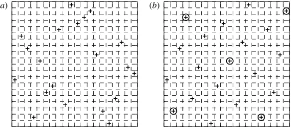
The definition of ‘uniform coverage’ is by no means obvious and a substantial body of literature exists on the subject—here we work with the optimality criterion of Morris & Mitchell (1995). According to this, the plan with the best space-filling properties is that which maximizes the smallest distance between any pair of points within the sample (several additional ‘tie-breaker’ criteria are given in case of multiple optima). Additionally, we restrict our search to a class of plans known as Latin Hypercubes (LH;McKayet al. 1979), which are built to ensure uniformly spread projections of all points on all axes (figure 5a shows a random LH). We thus generate an initial Morris–Mitchell optimal LH planXc. A more interesting question is how do we select anne-element subsetXeofXc, where the expensive simulations are to be run? Again, we wish to cover the parameter space evenly and hence turn to the Morris–Mitchell criterion, but this time we are dealing with a limited, discrete parameter space and thus the problem becomes a combinatorial one. Since selecting the subset that satisfies this is an NP-complete problem and an exhaustive search would have to examine

ncCneZnc!=ne!ðncKneÞ! subsets (clearly infeasible for all but very moderate

cardinalities), here we use an exchange algorithm to select Xe (Cook &

Nachtsheim 1980).

–10 –8 – 6 – 4 –2 0 2 4 6 8 10 0

1000 2000 3000 4000 5000 6000 7000 8000

B 2

d

Figure 4. Variances^2das the cheap function coefficientBis altered.s^ 2

d;reduces to 0 as the difference

We start from a randomly selected subsetXeand calculate the Morris–Mitchell criterion. We then exchange the first pointxðe1Þwith each of the remaining points in Xc\Xeand retain the exchange that gives the best Morris–Mitchell criterion. This process is repeated for each remaining pointxðe2Þ.xðne eÞ. A number of restarts from different initial subsets can be employed to avoid local optima. Figure 5bshows a Morris–Mitchell optimal LH with a subset chosen using this exchange algorithm.

A rule of thumb for the number of points that should be used in the sampling plan is n_Z10k. When using a particularly cheap analysis, nc may be rather greater than this, allowing us to build a more accurate model, and if the relationship between fc and fe is simple, ne may be somewhat fewer—the advantage of the co-kriging method. We will return to this subject in §7.

5. Co-kriging based optimization

In order to confirm and enhance the predictions of a surrogate model, it is usual to update the model with new evaluations in promising areas. Co-kriging (and kriging) treats the value of the function at x as if it were the realization of a Gaussian random variable Y(x), with a probability density function

1 ffiffiffiffiffiffi 2p p

sðxÞexpK 1 2

YeðxÞKy^_eðxÞ

sðxÞ

2

;

with mean given by the predictor, y^eðxÞ (equation (3.11)) and variance, s2(x) (equation (3.12)). This allows us to model our uncertainty about the predictions we make. The most plausible value atxisy^eðxÞ, with the probability decreasing asYe(x) moves away fromy^eðxÞ. Since there is an uncertainty in the value ofy^eðxÞwe can calculate the expectation of it being an improvement,I_ZminfyegKYðxÞ, on the best value calculated so far as

E½IðxÞZ ðN

KN

maxfminfyegKYeðxÞ;0gfðYeðxÞÞdYe

Z ð

minfy_egKy^_eðxÞÞF

minfyegKy^eðxÞ

sðxÞ 0

@

1

ACsðxÞf

minfyegKy^eðxÞ

sðxÞ 0

@

1

A if sO0;

0 if sZ0;

8 > > < > > :

(a) (b)

whereF($) andf($) are the normal cumulative distribution function and probability density function, respectively. By maximizingE[I(x)] we can find the best new point at which to sample the design space. Note thatE[I(x)]_Z0 whens(x)_Z0 so that there is no expectation of improvement at a point that has already been sampled and therefore no possibility of re-sampling, which is a necessary characteristic of an updating criterion when using deterministic computer experiments, and guarantees global convergence; given that there is no possibility of re-sampling, as the number of updates based on the maximum E[I(x)] increases, the design space will become densely populated and so the global optimum will be found (Locatelli 1997).

(a) Co-kriging regression

When using multi-fidelity analyses, we can modify the interpolating co-kriging formulation in§3 such that each analysis can be regressed appropriately to filter any noise present in the data. Different levels of filtering may be required for each analysis. For example, data from an empirical low-fidelity computer code may be smooth and require no regression, but could be coupled to a discretized high-fidelity analysis that displays noise that must be filtered using regression. Conversely, a low-fidelity model may be discretized on a much coarser mesh, requiring a higher degree of regression than the high-fidelity code. In our regressing co-kriging formulation, we therefore employ two regression constants, lcand le. These are added to the leading diagonal of the correlation matrices to give the covariance matrixCCl,

s2cfJcðXc;XcÞCI_ðnc!ncÞl_cg rs2_cfJ_cðX_c;X_eÞC

0ðncKne!neÞ

Iðne!neÞ

! lcg

rs2cfJcðXe;XcÞ r2s2cfJcðXe;XeÞCI_ðne!neÞl_cg

C 0_ðne!ncKneÞI_ðne!neÞ

lcg Cs2_dfJ_dðX_e;X_eÞCI_ðne!neÞl_eg 0

B B B B @

1 C C C C

A; ð5:1Þ

where I is an identity matrix and 0 a zero matrix. The values of lc and le are found along with the other hyper-parameters by maximizing equations (3.3) and (3.8). The regressing predictor is now

^

ye;rðxðneC 1Þ

ÞZm^CcTðCClÞK1ðyK1m^Þ; ð5:2Þ (subscript r denotes regression) with an estimated mean-squared error

(b) Co-kriging re-interpolation

We now show the derivation of a co-kriging error estimate that reflects the uncertainty in predicting the underlying trend of data, rather than the overall uncertainty, which includes any error in noisy data. The derivation, although naturally complicated by multiple sets of data and regression constants, follows the same theme as for kriging re-interpolation (Forrester et al. 2006b). As mentioned above, to eliminate the error in the noisy data, we need to calculate the error of an interpolation through a regressed set of data. The column vectors of regressed cheap and expensive data are found from equations (2.3) (with the addition of the regression constant) and (5.2), and can be expressed as

^

yc;rZ1mc^ CJcðJcC^lcIÞK1ðycK1mc^Þ and

^

ye;rZ1ðne!1Þm^Cfcðx

ð1Þ

e Þ T

;_.;cðxðneÞ

e Þ T

gTðCClÞK1ðyK1_ðn!1Þm^Þ;

where the MLEs for the hyper-parameters are those found for the co-kriging model. Note that only thes2terms in equation (3.12) depend ony. We therefore need to substitute y^c;r into equation (3.5) and y^e;r into equation (3.9). Beginning with s^2c,

^

s2c;riZ

ðycK1m^_cÞðJ_cCl_cIÞK1J_cðJ_cCl_cIÞK1ðy_cK1m^_cÞ

nc

ð5:4Þ

(subscript ri denotes re-interpolation). Note that if lcZ0, thens^2c;riZs^ 2

c. To find

^

s2_d;ri, we substitutey^e;r and y^c;r into equation (3.7) to give drZ1ðne!1Þm^Cfcðx

ð1Þ

e ÞT;.;cðxðne eÞÞTgTðCClÞK1ðyK1_ðn!1Þm^Þ

Kr^ 1mc^ CJcðXeÞðJcðXeÞClcIÞK1ðycðXeÞK1mc^Þ

:

This is substituted into equation (3.9) in place of d (again, note that if leZ0 then s^2_d;riZs^2_d). The expressions for s^2c;ri and s^2d;ri can now be substituted into equation (3.12) to find the re-interpolation error estimate that reduces to 0 at Xe. With the errors due to noisy data removed, the estimated error of the predicted smooth trend is typically very small when compared with an interpolating model. This can lead to problems with floating-point underflow when calculating

E[I(x)]. A scheme for avoiding this problem is presented in appendix B.

6. Example problem

with viscous coupling (approx. 2 min per drag evaluation). We aim to minimize drag/dynamic pressure (D/q) for a fixed lift (determined by a wing weight calculated by Tadpole).

To allow visualization of the design landscape, we limit the search to the four variables that have the most impact on drag: area,S; aspect ratio, ; sweep, L; and inboard taper ratio,Tin(these variables were shown to be the most dominant

by Keane (2003)). The Tadpole and VSaero design landscapes are shown using

hierarchical axis plots in figures6and7. With the fast empirical drag estimation provided by Tadpole, we have been able to build a high-resolution plot from 114Z14 641 runs of the code in 2.3 hours, while using the slower physics-based

VSaero we have produced a low-resolution plot using 32!112_Z1089 evaluations in 34.5 hours.4 Each tile of the plots shows D/q for S₂{150, 250}m2 and

2{6, 12} for a fixedLand Tin.LandTinvary from tile to tile, with the value at the lower left corner of the tile representing the value for the entire tile. The blank portions offigure 7 are regions where VSaero has failed to return a result for unusual geometries that lead to extreme flow regimes.5It is seen that the two codes produce results that follow the same general trend of lowerD/qfor higher and Tin, but the global optimum of the VSaero landscape goes against this general trend, with the lowestD/qatTinZ0.55.Zdwill not, therefore, be a trivial function as in our one-variable example but, since the cheap and expensive landscapes have the same general trend, should be simpler thanZe.

For this problem, we start with an initial Morris–Mitchell sampling plan for Xcof 100 points (notencO10k), to which a kriging model is fitted. A comparison of 100 further Tadpole calculations with predictions from the kriging model yields a high correlation coefficient of 0.96, indicating that the cheap code is approximated well. A subset of neZ20 points (note ne!10k) is selected (using the exchange algorithm) from which to build the initial co-kriging model.Xcand Xeare shown infigure 6. Despite the apparent sparseness of theXedata, a good initial co-kriging prediction of the VSaero landscape is obtained, with a correlation coefficient of 0.96 when compared with the 112!32 VSaero dataset. We follow an iterative process of updating the co-kriging model with new VSaero and Tadpole data at max{E[I(x)]} and retuning hyper-parameters until the optimum is found. Sincencis large and the correlation with independent data is high, we do not expect the Tadpole landscape to be altered unduly by updates. The GA-based tuning of qc and lc requires a large number of computationally intensive inversions of the large nc!nc covariance matrix. We therefore save time by limiting our re-tuning of the cheap hyper-parametersqcand lcto every 10 updates, while we re-tune qeand leat each step.

The co-kriging method is compared with a max{E[I(x)]} search of a kriging model built using only the VSaero data. A D/q that improves on the minimum from the previously computed 32!112set of data plus one standard deviation of the noise exhibited by the VSaero results (found from 10 VSaero evaluations of the same design with small perturbations), D/qZ2.57C0.027, is used as a stopping

4

Generating such plots would, of course, not be possible in most cases due to the high computational cost. Here we have computed this large quantity of data for illustrative purposes.

5_{In our co-kriging and kriging-based searches, we have directed the search away from regions of}

failure by inputing penalized values of y^eðxeÞCs2ðxeÞ when VSaero fails to return a result

2.5 3.0 3.5 4.0 4.5

25 27 29 31 33 35 37 39 41 43 45 0.40

0.43 0.46 0.49 0.52 0.55 0.58 0.61 0.64 0.67 0.70

sweep (deg.)

inboard taper ratio

Figure 6. Tadpole calculatedD/qwith a typical sampling plan.Xc(Tadpole evaluations) are shown as

dots and are circled at locations ofXe(VSaero evaluations). Red circles, failed VSaero simulations.

2.5 3.0 3.5 4.0 4.5 5.0

25 27 29 31 33 35 37 39 41 43 45 0.40

0.43 0.46 0.49 0.52 0.55 0.58 0.61 0.64 0.67 0.70

sweep (deg.)

inboard taper ratio

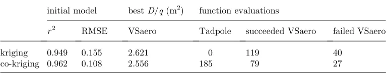
criterion in both cases, i.e. similar quality answers are achieved from both the searches, allowing a direct comparison of the effort involved. We also limit the size of the kriging and co-kriging models to a maximum of 200 VSaero calculations. Beyond this, the time required for tuning the model becomes equivalent to the time required to run VSaero. Results, averaged over five searches from sampling plans produced using different random number seeds, are shown intable 1.

The co-kriging based search consistently outperforms the kriging-based search; finding better optima for reduced numbers of VSaero evaluations and with fewer failed simulations. The initial prediction of the kriging model is almost as accurate as the co-kriging model (see correlation and RMSE in table 1), but the greater coverage of data in the co-kriging model leads to a better selection of successful update points in promising regions, as seen infigure 7, which shows the distribution of update evaluations for a typical search. Moreover, the co-kriging updates are concentrated in regions of good designs, while the kriging updates are more widespread because, as there is a sparsity of data, there is high error and therefore high expectations of improvement in many areas (i.e. there is an emphasis on exploration over exploitation).

Only discrete values ofLandTincan be displayed infigure 7and these design variables are rounded to the nearest 28 and 0.03 respectively, for the purpose of visualization. It should be borne in mind that there is, in fact, a distribution of designs between tiles. The reader should also appreciate that, although the major axis is much larger than the axes of the individual tiles, they both represent the same variation across a variable. Thus, although there seems to be a wide distribution of update points acrossL and Tin, for the co-kriging updates these points represent tight clusters in regions of optimal feasible designs.

In §3 we discussed the use of two regression constants lc and ld in the co-kriging formulation. The final MLEs of these hyper-parameters for the search infigure 7werelc^ Z1:2!10K6_andld^

Z6:5!10K3_{. These values agree with our} intuition that data from an empirical code (Tadpole) will be smooth and require little regression, i.e. a very small l^c, and data from a dicretized physics-based code (VSaero) will be noisy and require smoothing, i.e. a larger ^ld.

7. Discussion

Our results demonstrate that correlating analyses at multiple levels of fidelity can enhance the accuracy of a surrogate model of the highest level of analysis. This correlated model can be used to find optimal solutions more quickly. We have Table 1. Performance comparison for the four-variable transonic wing problem. (Averaged over

five searches.)

initial model bestD/q(m2) function evaluations

r2 _{RMSE VSaero Tadpole succeeded VSaero failed VSaero}

kriging 0.949 0.155 2.621 0 119 40

presented a global optimization strategy using a co-kriging based method that allows for varying levels of noise filtering across multi-fidelity analyses and which converges towards the global optimum using expected improvement maximization.

We have shown a co-kriging based optimization using two levels of CFD code fidelity. The methods are extendable to multiple levels and there are many other examples of analyses that may be coupled. Here, both codes are predicting the same quantity (drag) but, as long as there is a useful correlation, the analyses may be related to completely different quantities as is the case with the work ofHevesiet al.

(1992), which correlated precipitation with elevation: two different but obviously

correlated quantities. Often only one form of analysis is available, although this may come in varying levels of fidelity. For example,Kennedy & O’ Hagan (2000)used different finite-element mesh resolutions to produce cheap and expensive results.

Forresteret al. (2006a)showed that partially converged CFD simulations correlate

well with their converged counterparts. The convergence could be stopped at any number of points, thus providing many levels of fidelity.

In§4 we discussed the choice ofncand nebased on using more or fewer points than ann_Z10krule of thumb. In the example problem, we checked that the model built using our choices ofncandnewas accurate by assessing the correlation with a second set of data. Naturally the number of points required is problem dependent and additional validation data may be too expensive to compute. A possible way to reduce computational effort in situations when the cost offcis considerable is to start with a very low nc and add data at points where the estimated error is maximized until an accurate cheap model is obtained. Model accuracy may be assessed using a leave-one-out cross-validation procedure. This method will produce a space-filling design with nccontrolled by the desired model accuracy. Maximum expected improvement updates could then proceed starting from an initial sample as small as neZ2, though it may be advantageous to follow a maximum error update strategy until an accurate model is produced.

This work has been supported by EPSRC grant code GR/T19209/01.

Appendix A

To derive the co-kriging predictor, we follow a method similar to that for ordinary kriging. The basis of this method is that we wish our prediction of a new expensive point to be consistent with the observed data and the MLEs for the hyper-parameters. We therefore augment the observed data with a predicted value and maximize the likelihood of this augmented dataset by varying our prediction while keeping the hyper-parameters fixed. This gives us an MLEy^e xðneC1Þ

.

The augmented dataset is defined as X~_ZfXTc XeTxðneC1ÞTgT and

~

y_ZfyTc yTe yðneC1Þg T

, with covariance matrix C~ given by ^

s2

cJcðXc;XcÞ r^s2cJcðXc;XeÞ r^s2cjcðXc;xðne

C1Þ Þ

r^s2cJcðXe;XcÞ r2cs^2cJcðXe;XeÞC^s2dJdðXe;XeÞ r^s2cjc Xe;xðne

C1Þ

C^s2djd Xe;xðne

C1Þ

r^s2cjcðXc;xðneC1ÞÞT r^s2cjcðXe;xðneC1ÞÞTC^s2djdðXe;xðneC1ÞÞT r2s^2cC^s2d 0 B B @ 1 C C A

which, definingc as a column vector of the covariance ofX and xðneC1Þ_{, can be} expressed as

~

C_Z C c

cT r2s^2cCs^2_d !

: ðA 1Þ

In equations (3.3) and (3.8) it is seen that only the last term of the ln-likelihood contains the sample data, and hence to find an MLE y^eðxðneC1ÞÞ we need to maximize

K 1

2ðy~K1mÞ T_~

CK1

ðy~K1mÞ;

which may be expressed as

K 1 2

yK1^m

^

yeðxðneC1ÞÞKm^ !T

C c

cT r2cs^2cCs^2_d !K1

yK1m^

^

yeðxðneC1ÞÞKm^ !

: ðA 2Þ

The inverse of the augmented covariance matrix C~K1 is found using the partitioned inverse formula (Theil 1971)

CK1

CCK1cðr2s^2_cCs^2_dKcTCK1cÞK1cTCK1 KCK1cðr2s^2_cCs^2_dKcTCK1cÞK1

Kðr2s^2_cCs^_d2KcTCK1cÞK1cTCK1 ðr2s^2_cCs^2_dKcTCK1cÞK1 !

:

ðA 3Þ

Substituting (A 3) into (A 2) and ignoring terms without ^yeðxðneC1ÞÞ we obtain K1

2ðr2_s^2

cCs^2_dKcTCK1cÞ

ðy^eðxðne C1Þ

ÞKm^Þ2

C

cTCK1_ðy K1^mÞ ðr2_s^2

cCs^2_dKcTCK1cÞ

ðy^eðx

ðneC1Þ

This expression is maximized by taking the derivative with respect toy^e xðneC1Þ

and setting it to 0, K1 r2_s^2

cCs^2_dKcTCK1c

ðy^eðx

ðneC1Þ

ÞKm^ÞC

cTCK1_ðy K1^mÞ ðr2_s^2

cCs^2_dKcTCK1cÞ

Z0: ðA 5Þ

Solving for y^eðxðneC1ÞÞ now gives

^ yeðxðneC

1Þ_Þ

Zm^CcTCK1ðyK1m^Þ: ðA 6Þ For the estimated mean-squared error in this prediction, we again turn to

Jones (2001)for our method of derivation. It is argued that our MLEy^e xðneC1Þ

is more accurate if the likelihood has a definite maximum, i.e. a high curvature. Conversely, if different values of y^e xðneC1Þ

have similar likelihoods the MLE is less accurate. The error in the predictor is therefore inversely related to the curvature (the second derivative with respect to ^ye xðneC1Þ

of the augmented likelihood. We have already found the first derivative in equation (A 5) and taking the derivative and inverse of this equation we obtain

s2ðxÞ_zr2s^2cCs^2_dKcTCK1c: ðA 7Þ This equation is not precisely the classically derived formula, which includes an extra termð1K1TCK1_cÞ2_=cT_CK1_{c. However, this extra term is so small that it} can safely be neglected.

Appendix B

The expected improvement (equation (5.1)) is typically calculated as

ðminfyegKy^_eðxÞÞ 1 2C

1 2erf

minfyegKy^_eðxÞ ffiffiffi

2 p

sðxÞ !

" #

C

sðxÞ ffiffiffiffiffiffi 2p

p exp K

ðminfyegKy^eðxÞÞ2 2s2_ðxÞ

: ðB 1Þ

When using re-interpolation, s(x) is typically small and so erf($)/K1 and exp($)/0. This often leads to floating-point underflow andE[I(x)]Z0. Using the

substitutionaZðminfyegKy^eðxÞÞ= ffiffiffi 2 p

sðxÞ, whena/K1, erf(a) can be expressed using a Maclaurin series expansion and the first term of (B 1) becomes

ðminfyegKy^_eðxÞÞ 1

2pffiffiffipexpðKa 2

ÞX

N

nZ0

ðK1Þnð2nK1Þ!!

2n a

Kð2nC1Þ

" #

:

Note that exp(Ka2) appears in the second term in (B 1) and thereforeE[I(x)] can now be expressed as

ðminfyegKy^_eðxÞÞ 1 2pffiffiffip

XN

nZ0

ðK1Þnð2nK1Þ!!

2n a

Kð2nC1Þ C

sðxÞ ffiffiffiffiffiffi 2p p

" #

!exp K

ðminfyegKy^_eðxÞÞ2 2s2_ðxÞ

We can now take natural logarithms and lnE[I(x)] can be searched by the optimizer without problems with floating-point underflow.

References

Cook, R. D. & Nachtsheim, C. J. 1980 A comparison of algorithms for constructing exact D-optimal designs.Technometrics22, 315–324. (doi:10.2307/1268315)

Cousin, J. & Metcalf M. 1990 The BAE Ltd. transport aircraft synthesis and optimization program. InAHS, and ASEE, Aircraft Design, Systems and Operations Conference, Dayton, OH, 17–19 September 1990.

Forrester, A. I. J., Bressloff, N. W. & Keane, A. J. 2006aOptimization using surrogate models and partially converged computational fluid dynamics simulations.Proc. R. Soc. A462, 2177–2204. (doi:10.1098/rspa.2006.1679)

Forrester, A. I. J., Keane, A. J. & Bressloff, N. W. 2006bDesign and analysis of ‘noisy’ computer experiments.AIAA J.44, 2331–2339. (doi:10.2514/1.20068)

Forrester, A. I. J., So´bester, A. & Keane, A. J. 2006cOptimization with missing data.Proc. R. Soc. A462, 935–945. (doi:10.1098/rspa.2005.1608)

Hevesi, J., Flint, A. & Istok, J. 1992 Precipitation estimation in mountainous terrai using multivariate geostatistics. Part II: isohyetal maps.J. Appl. Meteorol.31, 677–688. (doi:10.1175/ 1520-0450(1992)031!0677:PEIMTUO2.0.CO;2)

Jones, D. R. 2001 A taxonomy of global optimization methods based on response surfaces.J. Global Optim.21, 345–383. (doi:10.1023/A:1012771025575)

Keane, A. J. 2003 Wing optimization using design of experiment, response surface, and data fusion methods.J. Aircraft40, 741–750.

Kennedy, M. C. & O’Hagan, A. 2000 Predicting the output from complex computer code when fast approximations are available.Biometrika87, 1–13. (doi:10.1093/biomet/87.1.1)

Krige, D. G. 1951 A statistical approach to some basic mine valuation problems on the Witwatersrand. J. Chem. Metallurg. Min. Eng. Soc. S. Afr.52, 119–139.

Locatelli, M. 1997 Bayesian algorithms for one-dimensional global optimization.J. Global Optim.

10, 57–76. (doi:10.1023/A:1008294716304)

Maskew, B. 1982 Prediction of subsonic aerodynamic characteristcs: a case for low-order panel methods.J. Aircraft19, 157–163.

Matheron, G. 1963 Principles of geostatistics.Econ. Geol.58, 1246–1266.

McKay, M. D., Beckman, R. J. & Conover, W. J. 1979 A comparison of three methods for selecting values of input variables in the analysis of output from a computer code.Technometrics 21, 239–245. (doi:10.2307/1268522)

Morris, M. D. 1991 Factorial sampling plans for preliminary computational experiments. Technometrics33, 161–174. (doi:10.2307/1269043)

Morris, M. D. & Mitchell, T. J. 1995 Exploratory designs for computer experiments.J. Stat. Plan. Infer.43, 381–402. (doi:10.1016/0378-3758(94)00035-T)