Optimal Control and Guidance for Homing and Docking
Tasks using an Autonomous Underwater Vehicle
Pakpong Jantapremjit and Philip A. Wilson
Fluid-Structure Interactions Research Group, School of Engineering Sciences University of Southampton, Southampton, United Kingdom
{pakpong9, Philip.Wilson}@soton.ac.uk
Abstract— This paper presents the results of a control and guidance strategy for homing and docking tasks using an au-tonomous underwater vehicle. An optimal high-order sliding mode control via state-dependent Riccati equation approach is introduced providing a robustness of motion control including elimination of chattering effect for decoupled systems of an AUV. Motion planning for a docking is introduced. The average vector field based on an artificial potential field method gives a desired trajectory using existing information from ocean network sensors. It provides a guidance for an AUV to follow the path to a required position with final desired orientation. A Line-of-Sight method is used for an AUV to follow the predefined path. In order to improve a docking manoeuver, a switched weight technique is proposed for controlling a vehicle’s path and final stage docking.
Index Terms—AUV, Homing, Docking, Sliding Mode Control, State-dependent Riccati Equation.
I. INTRODUCTION
Remotely Operated Vehicles (ROVs) and Unmanned Un-derwater Vehicles are useful for many unUn-derwater operations such as collecting biological and mineral resources, however there are some limitations for those vehicles during long-term operations. Consequently an Autonomous Underwater Vehicle (AUV) which is able to make decisions and take control actions more accurately and reliably without human intervention is an alternative to humans especially in long-term underwater complex tasks. Examples of such operations are seabed mapping and surveying, studying underwater and under-ice environments. Although studies have been made of AUVs over the past thirty years [1], still AUV technology limitations remain. Due to the current state of computa-tional capability and data storage capacity, the technology can marginally provide fair speed and efficiency including well-established software developments. Energy storage and power consumption are critical factors for all long-term operations. Its short operational periods limit scopes of each undersea exploration. In long-term experimentation, a vehicle should be able to operate continuously for 24 hours a day. However most underwater vehicles are typically capable of short-term operation. Vehicles require both software and hardware to be turned off before its batteries can be manually recharged or replaced. To overcome the limitations of the onboard battery, data transfer and sensor ranges, a floating docking platform is required to provide a large scope of potential missions. A focus on docking operations allows a vehicle to recharge its
own battery and to exchange information before continuing its normal operations. To be able to perform its docking mission accurately, the guidance, navigation and control system must be reliable. There are many issues in determining the control aspects during the docking stages of missions.
The paper is organised as follows: Section II provides a dynamics model of a 6-DOF AUV. The standard sliding mode and optimal high-order sliding mode controller are given in section III and IV, respectively. In section V, a predefined trajectory for homing and docking using a vector field method based is proposed. The final section contains the conclusion and further works.
II. MODEL OF THEDYNAMICS OF ANAUV The system dynamics of AUVs are highly nonlinear, coupled and time varying which comes from many parameters, such as hydrodynamic drag, damping and lift forces, Coriolis and centripetal forces, gravity and buoyancy forces and forces from thrusters [2]. Attitude representation of our kinematic AUV model in the global reference frame is defined using Euler angles. The kinematic equation is thus written as,
˙
η=Rν(η)ν=
Rν1(η) 0
0 Rν2(η)
ν1 ν2
(1)
where Rν1(η) is the rotation matrix from the body frame to the inertial frame, and Rν2(η) is the angular velocity transformation from the body frame to the inertial frame, ν ∈ R6×1 is the vector of the linear and angular velocity of a
vehicle in the body-fixed frame, andη ∈R6×1 be the vector of position and attitude of a vehicle in the inertial frame,
ν = [ν1,ν2]T = [u, v, w, p, q, r]T η = [η1,η2]T = [x, y, z, φ, θ, ψ]T
The 6-DOF dynamic model of the AUV is derived from the Newton-Euler equation of motion of a rigid body in the fluid. The dynamic model is given by,
Mν˙ +C(ν)ν+D(ν)ν+g(η) =τ . (2)
whereM is an AUV inertia matrix (including added mass), C(ν)is the matrix of Coriolis and centripetal terms (including added mass effects), D(ν) is a hydrodynamic damping and lift matrix of the AUV,g(η)is the gravitational and buoyancy force and moment vectors, and τ is an external force and moment input.
Proceedings of the 2007 IEEE
III. SLIDINGMODECONTROL
Many studies have been undertaken in order to correct errors in attitude control including [3], [4]. Most stability schemes are formulated based on the Lyapunov method which provides ranges of positive stable gains for control law. Sliding mode control (SMC) which is a nonlinear controller provides excellent stability, robustness and disturbance rejection char-acteristics [5]. It is categorised as a variable structure control system [6] which has been studied in the Soviet Union for many years.
A. Sliding Surface
Consider the state space of a nonlinear system,
˙
x=Ax+Bu+f(x). (3)
wherexis the state vector,Ais the system matrix,Bthe input matrix,uthe inputs of the system andf(x)is the unknown function representing the model uncertainty and disturbances that would cause the system to deviate from its equilibrium point. The sliding surface is designed so that the surface tends to and converges to zero when it satisfies the Lyapunov stability criterion [5] thus the problem of tracking defined as x≡xd is equivalent to that of remaining on the surface for all time t > 0. A time-varying sliding surface σ which is suggested in [2] is defined as,
σ=hTx˜=hT(x−xd). (4)
wherex˜is tracking error vector,xdis desired trajectory vector
and h is the right eigenvector of the desired closed loop system. Given the candidate Lyapunov functionV(σ) =12σ2, then its derivative must satisfy,
˙
V(σ) =σσ˙ ≤0,
The condition when sliding surfaceσ= 0andσ˙ = 0is reached in a finite time if,
˙
σσ≤ −kσsgn(σ),
andsgn(σ) is a signum function. The control inputs can be regarded as that for the nominal plant and for the uncertainty of model parameter therefore it can be described in the following feedback control law,
u=ueq+usw=−kTx+usw, (5)
wherekis the feedback gain vector obtained from pole place-ment or linear quadratic differential equation. Differentiating (4) with respect to time and substituting with (3) and (5), gives
˙
σ=hT(Acx+busw+f(x)−x˙d), (6)
where
Ac=A−bkT,
The switching control law can be therefore chosen as,
usw= 1
hTb(h
Tx˙
d−hTf(x)−kσsgn(σ)), (7)
The control law of sliding mode is generally given,
u=ueq−Kσsgn(σ). (8)
whereueq is an equivalent control. Kσ is a constant,
corre-sponding to the maximum value of the controller input.
B. Chattering
Chattering is caused by a signum function, thus the switch-ing action may cause the system response oscillatswitch-ing about the zero sliding surface in high frequency mode. It can cause wear in the actuators. Reducing the chattering, a thin boundary layer of thickness around the switching surface is proposed in [5],
u=ueq−Kσsat(
σ
Φ). (9)
where the constant Φ defines the thickness of the boundary layer and sat(σ
Φ) is a saturation function. Furthermore an improvement to the behaviour, a hyperbolic tangent function is thus replaced to give a smoother response [7]. This term acts like a low pass filter so it becomes,
u=ueq−Kσtanh(
σ
Φ). (10) The rˆole of the sliding mode controller is to drive the system towards the sliding surface and keep it on the sliding surface. The sliding mode is a robust control design therefore it is able to improve a capability to track the desired state of the AUV modelling. Decoupled models of an AUV are discussed in the following section.
Ŗ ś ŗŖ ŗś ŘŖ Řś řŖ řś ŚŖ Ȭŗś
ȬŗŖ Ȭś Ŗ ś ŗŖ ŗś
ȱǻǼ
ȱȱ
δ
ȱǻǼ
Ŗ ś ŗŖ ŗś ŘŖ Řś řŖ řś ŚŖ ȬŗŖ
Ȭś Ŗ ś ŗŖ ŗś ŘŖ
ȱǻǼ
ȱȱ
ǰȱ
δ
ȱǻǼ
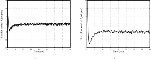
[image:2.612.322.568.447.543.2](a) (b)
Fig. 1. Control Effort for Heading Subsystem (a) with Disturbance
and for Depth Subsystem (b) with Disturbance.
C. Decoupled Subsystems
1) Heading Subsystem: The heading subsystem presents the steering of the AUV in the X-Y plane. The control input commands deflection of rudder. The heading subsystem comprises the sway velocityv, the yaw raterand the heading angle ψ, and the rudder deflection δr. Assuming an AUV
moving forward with constant speedu0, the equation of motion for heading is given as follows,
⎡
⎣mxmG−−YNv˙ v˙ mxIzzG−−NYr˙r˙ 00
0 0 1
⎤ ⎦ ⎡ ⎣vr˙˙
˙
ψ
⎤ ⎦
=
⎡
⎣NYvr NYrr−−mxmuG0u0 00
0 1 0
⎤ ⎦ ⎡ ⎣vr
ψ
⎤
⎦+
⎡ ⎣NYδδ
0
⎤ ⎦δr
(11) The sliding surface for heading subsystem is defined,
σ1 = hT1(x−xd),
= s1(v−vd) +s2(r−rd) +s3(ψ−ψd),
and the heading control law becomes,
u1 = −k1v−k2r+ 1
hT1b1[−kσ21tanh( σ1
Φ)].
where a feedback gain [k1, k2, k3]T for heading subsystem is determined by pole placement method.
2) Depth Subsystem: The depth subsystem presents the depth motion of the AUV in theX-Z plane. The control input commands deflection of sternplanes or bowplanes. The depth subsystem comprises the heave velocity w, the pitch angular velocity q, the pitch angleθ, the depth z and the sternplane deflection δs. Similarly, assuming an AUV moving forward
with constant speed u0, the equation of motion in heave and pitch is given as follows,
⎡ ⎢ ⎢ ⎣
m−Zw˙ mxG−Zq˙ 0 0
mxG−Mw˙ Iyy−Mq˙ 0 0
0 0 1 0
0 0 0 1
⎤ ⎥ ⎥ ⎦ ⎡ ⎢ ⎢ ⎣
˙
w
˙
q
˙
θ
˙
z
⎤ ⎥ ⎥ ⎦
=
⎡ ⎢ ⎢ ⎣
Zw Zq−mu0 0 0 Mw Mq−mxGu0 −zBW 0
0 1 0 0
0 0 −u0 0
⎤ ⎥ ⎥ ⎦ ⎡ ⎢ ⎢ ⎣
w q θ z
⎤ ⎥ ⎥
⎦+
⎡ ⎢ ⎢ ⎣
Zδ Mδ
0 0
⎤ ⎥ ⎥ ⎦δs
(12) The sliding surface for depth subsystem is expressed,
σ2 = hT2(x−xd),
= s1(w−wd) +s2(q−qd) +s3(θ−θd) +s4(z−zd),
and the heading control law becomes,
u2 = −k1w−k2q−k4z+ 1 hT
2b2
[−kσ22tanh(σ2 Φ)].
where a feedback gain[k1, k2, k3, k4]Tfor depth subsystem is determined by pole placement method.
IV. OPTIMALSLIDINGMODECONTROL
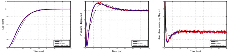
This section presents optimal sliding mode control via a state-dependent Riccati equation technique. The high-order sliding mode control is introduced in order to eliminate the effect of chatter. An approximation of the sliding mode control effort for subsystems is formulated via the state-dependent Riccati equation. Comparative studies of control law between control techniques using computer simulation are illustrated as shown in Fig. 2 and 3. The performances have been improved. Chattering effect is eliminated while retaining the main characteristic of the standard SMC.
A. High-order Sliding Mode Control
Standard sliding mode controls have proved high accuracy and robustness with respect to external disturbances, however they also have drawback: the so-called chattering phenomenon. It may excite high frequency vibrations which degrades the performance of the control system. High-order sliding mode controllers (HOSMC) have been currently developed to avoid this chattering [9]. HOSMC acts on the high-order time derivatives. Whilst the method keeps the main advantage of the standard sliding mode, it also eliminates the chattering. A number of applications in this topic can be found in [10], [11]. Consider a simple dynamic system,
˙
x = a(t,x) +b(t,x)u, (13a)
σ = σ(t,x), (13b)
wherex∈Rn,a,bandσ∈Rn+1→Rare unknown smooth
functions,u∈R. The standard sliding mode is satisfied when the sliding surface is reached in a finite time,σ= ˙σ= 0. Now following [12], it can be seen that,
σ(r)=h(t,x) +g(t,x)u, (14) whereg(t,x)andh(t,x)are uncertain functions that bound,
|h(t,x)| < Φ
0 < Γm<g(t,x) < ΓM
whereΦ,ΓmandΓM >0. Ther-thsliding mode (r-sliding)
[9] is determined by,
σ= ˙σ= ¨σ=· · ·=σ(r−1)= 0 Control laws can be expressed,
u1 = −kσsgn (σ) (15a)
u2 = −kσsgn( ˙σ+|σ|12sgn (σ)) (15b)
B. The State-Dependent Riccati Equation Method
The State-Dependent Riccati Equation (SDRE) is a well established, accepted and effective methodology [13] for the synthesis of control laws for nonlinear systems. Literature and application using SDRE technique are found in [14], [15]. Fundamentally the SDRE is derived to minimise the performance index,
J = 1
2
∞
t0
Ŗ ś ŗŖ ŗś ŘŖ Řś řŖ řś ŚŖ Ŗ
ŗŖ ŘŖ řŖ ŚŖ śŖ ŜŖ ŝŖ
ȱǻǼ
ȱȱǻǼ
Ȭ
Ŗ ś ŗŖ ŗś ŘŖ Řś řŖ řś ŚŖ ȬŖǯŗ
ȬŖǯŖś Ŗ ŖǯŖś Ŗǯŗ Ŗǯŗś ŖǯŘ ŖǯŘś Ŗǯř
ȱǻǼ
¢ȱ¢ȱǻȦǼ
Ȭ
Ŗ ś ŗŖ ŗś ŘŖ Řś řŖ řś ŚŖ Ȭŗś
ȬŗŖ Ȭś Ŗ ś ŗŖ ŗś
ȱǻǼ
ȱȱ
δ
ȱǻǼ
[image:4.612.111.504.52.144.2]Ȭ
Fig. 2. Comparison of Heading Control with Disturbance using SMC, HOSMC and SDRE-HOSMC techniques.
Ŗ ś ŗŖ ŗś ŘŖ Řś řŖ řś ŚŖ Ŗ
Ř Ś Ŝ Ş ŗŖ ŗŘ
ȱǻǼ
ȱǻǼ
Ȭ
Ŗ ś ŗŖ ŗś ŘŖ Řś řŖ řś ŚŖ ȬŘŖ
Ȭŗś ȬŗŖ Ȭś Ŗ ś
ȱǻǼ
ȱȱǻȦǼ
Ȭ
Ŗ ś ŗŖ ŗś ŘŖ Řś řŖ řś ŚŖ ȬŗŖ
Ȭś Ŗ ś ŗŖ ŗś ŘŖ
ȱǻǼ
ȱȱ
ǰȱ
δ
ȱǻǼ
Ȭ
Fig. 3. Comparisons of Depth Control with Disturbance using SMC, HOSMC and SDRE-HOSMC techniques.
with respect to the state x and control u subject to the nonlinear dynamic system which can be expressed in the State Dependent Coefficient (SDC) form, similar to a nonlinear form,
˙
x=Ax+Bu (17)
Solving the SDRE which is simply given by,
ATP+P A−P BR−1BTP+Q= 0 (18) Nonlinear feedback control law can be constructed as,
u = −Kx,
= −R−1BTPx. (19)
whereP > 0, Q is state-dependent weight matrix and R is control weight matrix.
V. HOMING ANDDOCKINGSTRATEGY
A. Review
In the long-term underwater application, docking operation is important for recharging power and transferring data which are limited by the on-board energy storage and on-board data storage. The general problem of accurately stabilising the position and orientation of the underwater vehicle is a key problem of docking task. In this section, a literature review for a docking task in the marine vehicle is explored. Kato and Endo [16] have presented a concept of docking guidance and control for unmanned submersibles at stationary platform by using fuzzy algorithms. Two steps are: coarse guidance based on fuzzy algorithms provides prearrangement of the vehicle to docking target and precise guidance based on sonar and transponders give a precise distance and target position and orientation. By using a short range position system, Evanset al.[17] have developed a precise docking guidance for ROV applicable of power recharging and data transferring. Since
position and orientation of AUV near a docking platform are accurately required, Feezoret al.[18] have proposed electro-magnetic homing systems for the AUV guidance. The AUV is equipped with sensors to follow magnetic fields transmitted from such a system into the docking entrance. Interestingly, biologically-inspired strategies for homing and docking have been considered by recent researchers [19], [20]. Visual based navigation of insects can be explained by the snapshot model [21] and Average Landmark Vector model (ALV) proposed by [19]. The docking strategy proposed in this paper using an AUV is inspired by these works.
B. Homing Strategy
The homing trajectory is modelled with a conventional artificial potential method. It is an approach that breaks up the free space into a fine grid which is then searched for a free path. Each grid element is assigned apotential, where the goal and neighbouring elements are assigned anattractivepotential and obstacles possess arepulsive potential. This ensures that the path created moves towards the goal while steering clear of any obstacles. Details can be found in [22]. With a use of acoustic sensor network such as Long-Based-Line (LBL), an AUV is therefore able to track the gradient field thus it reaches the minimum potential. Samples of home planning using conventional potential field method are shown in Fig. 4.
C. Docking Strategy
[image:4.612.110.501.181.273.2]Ŗ ŗ Ř ř Ś ś Ŝ ŝ Ş ş ŗŖ Ŗ
ŗ Ř ř Ś ś Ŝ ŝ Ş ş ŗŖ
Ŗ ŗ Ř ř Ś ś Ŝ ŝ Ş ş ŗŖ Ŗ
ŗ Ř ř Ś ś Ŝ ŝ Ş ş ŗŖ
[image:5.612.53.296.52.154.2](a) (b)
Fig. 4. Simulation results of home planning using potential field
method with (a) three obstacles (b) four obstacles. The◦and+in the
figure denote the starting points and home position of the trajectories.
docking velocity is kept within a safe range in order to avoid a possible serious impact between platform, a visual docking is a possible method that is used to perform a final docking. Similar to a method from the visual based navigation of insects [21], average landmark vector model [19] and conventional artificial potential field, an average vector field for predefined homing and docking trajectory provides more compact representation introduced in the following sections.
1) Average Vector Field: A potential field function at sensor networkNi is simply defined,
U(q) = ni=1Ni(q)− N(q) , ∇U(q) = −ni=1 Ni(q)− N(q) Ni(q)− N(q)
=−QT
i.
(20)
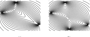
where a vector field q with unit length point towards sensor network Ni. Fig. 5 shows results of average vector field
distribution at sensor networks in the workspace. At least three sensors provide a clear valley thus it is helpful for the docking problem.
(a) (b)
Fig. 5. The level sets of the average vector field for (a) three sensor
nodes, (b) four sensor nodes. The• in the figure denote the sensor
location.
2) Switching Weighted Vector Field: To enhance the desired target achievement for improving a docking manoeuvre, a switching time varying weights is extended for two phased docking. The central sensor node is greater meaning for a vehicle to perform docking manoeuvre. Firstly, a vehicle is driven towards the middle of convex hull by using the first weight set1 and once the vehicle is aligned at the centre of valley and then a second set of weight2is applied for a final docking manoeuvre. The equation is,
Qi =
n
i=1
i(t) Ni(q)− N(q) Ni(q)− N(q)
, (21)
where i(t) is the weight of sensor node. According to switching weighted average vector field which is proposed for trajectory planning, the vector is computed,
q=
n
i=1
i(t)pi, (22)
Three sensor nodes are available to the AUV for position and orientation in the environment, so it is more convenient to compute the minimum potential force as,
∇Umin = min(∇U(q)). (23)
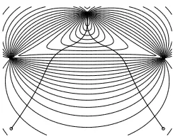
wheremin returns the minimum vector among all∇U. Min-imising∇Umin gives the goal of its minimum which is close to the target point. The minimisation point of the sum of potentials of each node will fall down to the valley area with respect to level set of |Q| and then converge to a minimum. The control algorithm starts determining the gradient of the potential functions related to all three sensor nodes as shown in Fig. 6(a) leading a trajectory of a vehicle approaching the target along the gradient flows toward a single minimum potential. Fig. 6(b) shows that robot approaching a valley where its potential field convert toward the minimum. Then, the control algorithm will lead a vehicle to archive both position and orientation along computed trajectory resulting a docking manoeuvre at docking station as shown in Fig. 6(c).
D. Line-of-Sight Path Following
The aim of path following is to follow a predefined path which is represented by a series of vehicle’s coordinates(x, y) joined by line segments. A number of techniques have been developed to solve this problem. The Line-of-Sight (LoS) guid-ance technique is intuitive and widely used in the application for path following of underwater vehicles both in 2D and 3D [2]. LoS law can be computed as,
ψLoS = atan2(yLoS−y, xLoS−x). (24)
[image:5.612.81.264.452.528.2]where the four quadrant atan2ensures thatψLoS ∈ −π, π . Simulation using MATLAB for predefined path following using LoS method a for docking task is illustrated. Fig. 7 shows simulation of trajectory using switching weight set. Fig. 8 shows simulation of trajectory following employing the constant and the switching weight set.
VI. CONCLUSIONS
¡ ¢
ř 1
1
1
Ř ř
¡ ¢
1
1
1
¡ ¢
1
1
1
[image:6.612.140.478.52.181.2](a) (b) (c)
Fig. 6. An AUV is influenced by three sensors. Sensors are represented by•. (a) Summing all vector fields, AUV is to determine
[image:6.612.111.233.237.335.2]the minimum potential force (b) AUV visits a valley where is around the centre area in the convex hull (c) After approaching closing to the target AUV is performing docking at the docking station.
Fig. 7. Trajectory planning using switching weight set giving a
smooth trajectory. The first weight set (0.8 , 0.8, 0.5) is used for a converge trajectory to a centre valley far from the sensor nodes. Then a time varying weight function give the smooth trajectory converge to a preparation of final docking orientation with the second set of weight (1, 1, 1.3) at the centre sensor node representing a docking station.
(a) (b)
Fig. 8. Path following simulations using LoS guidance of an AUV
model which predefined trajectory is generated by (a) constant weighted set (b) switching weighted set.
REFERENCES
[1] J. Yuh, “Design and control of autonomous underwater robots: A survey,” Autonomous Robots, vol. 8, pp. 7–24, 2000.
[2] T. Fossen,Guidance and Control of Ocean Vehicles. England: John
Wiley and Sons Ltd., 1994.
[3] D. Boskovic and M. Krstic, “Global attitude/position regulation for
underwater vehicles,”International Journal of Systems Science, vol. 30,
no. 9, pp. 939–946, 1999.
[4] P. Tsiotras, “New control laws for the attitude stabilization of rigid
bodies,”IFAC Symposium on Automatic Control in Aerospace, pp. 12–
16, 1994.
[5] J. Slotine and W. Li,Applied Nonlinear Control. New Jersey:
Prentice-Hall, Inc, 1991.
[6] V. Utkin, Sliding Modes and Their Application in Variable Structure
Systems. Moscow: MIR Publishers, 1978.
[7] C. Vuilmet, “High order sliding mode control applied to a heavyweight
torpedo,”Proceedings of 2005 IEEE Conference on Control
Applica-tions, pp. 61–66, 2005.
[8] A. Healey and D. Lienard, “Multivariable sliding mode control for autonomous diving and steering of unmanned underwater vehicles,” IEEE Journal of Oceanic Engineering, vol. 18, no. 3, pp. 327–339, 1993. [9] A. Levant, “Higher-order sliding modes, differentiation and
output-feedback control,”International Journal of Control, vol. 76, no. 76, pp.
924–941, 2003.
[10] D. Galzi and Y. Shtessel, “UAV formations control using high order
sliding modes,”Proceeding of the 2006 American Control Conference,
pp. 4249–4254, 2006.
[11] T. Salgado-Jimenez and B. Jouvencel, “Using a high order sliding modes for diving control a torpedo autonomous underwater vehicle,” Proceedings in OCEANS, vol. 2, pp. 22–26, 2003.
[12] A. Levant and L. Alelishvili, “Universal SISO sliding-mode controllers
with finite-time convergence,”IEEE Transactions on Automatic Control,
2001.
[13] D. Stansbery and J. Cloutier, “Position and attitude control of a
space-craft using the state-dependent riccati equation technique,”Proceedings
of the 2000 American Control Conference, vol. 3, 2000.
[14] A. Bogdanov, E. Wan, and G. Harvey, “SDRE flight control for X-Cell
and R-Max autonomous helicopters,”43rd IEEE Conference on Decision
and Control, vol. 2, pp. 1196–1203, 2004.
[15] W. Ren and R. W. Beard, “Constrained nonlinear tracking control for
small fixed-wing unmanned air vehicles,”American Control Conference,
pp. 4663–4668, 2004.
[16] N. Kato and M. Endo, “Guidance and control of unmanned, untethered
submersible for rendezvous and docking with underwater station,”
Pro-ceedings OCEANS ’89, vol. 3, pp. 804–809, 1989.
[17] J. Evans, K. Keller, J. Smith, P. Marty, and O. Rigaud, “Docking techniques and evaluation trials of the swimmer auv: an autonomous
deployment auv for work-class rovs,”MTS/IEEE Oceans Conference
Proceedings on An Ocean Odyssey, vol. 1, pp. 520–528, 2001. [18] M. Feezor, F. Sorrell, P. Blankinship, and J. Bellingham, “Autonomous
underwater vehicle homing/docking via electromagnetic guidance,” MTS/IEEE Conference Proceedings on Oceans, vol. 26, no. 4, pp. 547– 555, 1997.
[19] R. Moller, “Insect visual homing strategies in a robot with analog
processing,”Biological Cybernetics, pp. 231–243, 2000.
[20] R. Wei, R. Mahony, and D. Austin, “A bearing-only control law for stable
docking of unicycles,”IEEE/RSJ International Conference on Intelligent
Robots and Systems (IROS 2003), pp. 27–31, 2003.
[21] D. Lambrinos, R. Moller, T. Labhart, R. Pfeifer, and R. Wehner, “A
mobile robot employing insect strategies for navigation,”Robotics and
Autonomous Systems, pp. 39–64, 2000.
[22] O. Khatib, “Real-time obstacle avoidance for robot manipulator and
mobile robots,”The International Journal of Robotics Research, pp. 90–
[image:6.612.61.283.419.541.2]