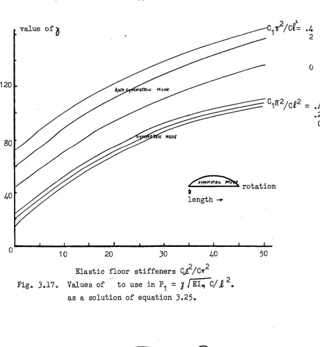
An approach to structural analysis

AN APPROACH TO STRUCTURAL ANALYSIS by

Anthony R. Kjar B.E.(Hons.)

submitted in partial fulfilment of the requirements for the degree of

Doctor of Philosophy, in the Faculty of Engineering

UNIVERSITY OF TASMANIA AUSTRALIA.

INDEX

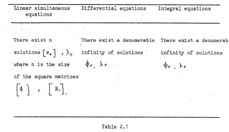
CHAPTER ONE Measuring geometry to obtain simple 1 mathematical models

CHAPTER TWO An outline of the instability problem 21

CHAPTER THREE _{A mathematical model for a through bridge 52}

CHAPTER FOUR Refinements of the mathematical model of 96

the through bridge

CHAPTER FIVE The design of through bridges 119

CHAPTER SIX Torsion

154

PREFACE

The purpose of this thesis is to present to the engineering profession a method of structural analysis which is peculiarly suited to the way engineers think. •The range and the power of structural analysis are extended by careful study of the actual deformations of structures, leading to the

formLulation of

simple mathematical models. The theme throughout this thesis is the deliberate effort to look for, and to describe characteristic shapes which define the deformed structure; general statements are

obtained similar to the historically valuable models which

used "plane sections remain plane" or "radial lines remain radial". Once an appreciation of the deformations of the structure is gained, the forces to sustain these deformations are then found easily.

This is one of the oldest approaches of engineering analysis, and the most powerful methods of analysis of structures have been along these lines, Men like Galileo, Parent, Navier, Bernoulli, and Ooidoimb developed an appreciation of structural behaviour by looking for simple geometric characteristics which would describe the deformed shape of the structure. (We may note also that Kepler's purely geometric study of the motions of the planets paved the way for Newton's formulation of his laws). And today p when one tries to visualize and calculate the deformations of a bent beam, it is difficult to improve upon the first overall approximation that plane sections remain plane.

the stresses, and hence the overall statical equilibrium of the structure can be evaluated. With this basis on which thoughts can be focussed, the laboratory and mathematical models can be improved to be a closer

representation of the real problem. This approach reduces the need to test full—size structures, as the geometric functional form acts as the geometric scaling factor. When full size testing is carried out, model tests are still a valuable means of providing a quick overall picture. This picture can then be used to determine which important geometric deformations should be measured. At present, full—size testing, although expensive, is still necessary as the relationships between the strength

and the size of the material remain unanswered. Nevertheless, improve-

ments

in this field can be made; for example R.E. Rowe (Ref. 1) has shown that concrete mixtures can be scaled to produce the same geometric crack pattern as would be expected in the full—size structure.

An engineer is frequently using approximate overall characteristics

of a simple model as a basis for obtaining further thoughts on the real problem. However, the inability to measure quickly the overall geometric deformations of a simple model has led to specialized full—size structural

tests, not by engineers, but by research workers. The aim of this thesis if to show how to use simple experimental studies to obtain simple,,.

mathematical models, and thus fulfil the sentiment expressed by Sir Alfred Pugsley (Ref. 2) that "Drawing and design office staffs can, and like to, play a part in the extension of their methods, and if they could do so directly, not only by theoretical but 1:y simple experiment, would welcome the opportunity".

The design of a through plate girder bridge is taken as the main

problem throughout this thesis in order to co—ordinate the whole. Existing mathematical models and methods of design are based on the ideas developed after the buckling failure of several through bridges

through bridges. An understanding of the problem is obtained from these model studies, and is used to develop a new mathematical model. The predictions of this new model are then compared with measurements

taken on a full—size bridge with strain gauge, spirit level, and rule,

and reasonable agreement is obtained. This new mathematical model is then used as the basis for recommendations concerning the design of through bridges made with light floors.

In Chapter One the author presents a case for measuring geometric

deformations as a means of obtaining a good functional form for the description of the structural problem. Simple and well known examples of stretched, bent, and twisted bars are chosen in order that the main features of the method are not lost in the process of mathematical manipulation.

Chapter Two begins with a detailed analysis of the structural

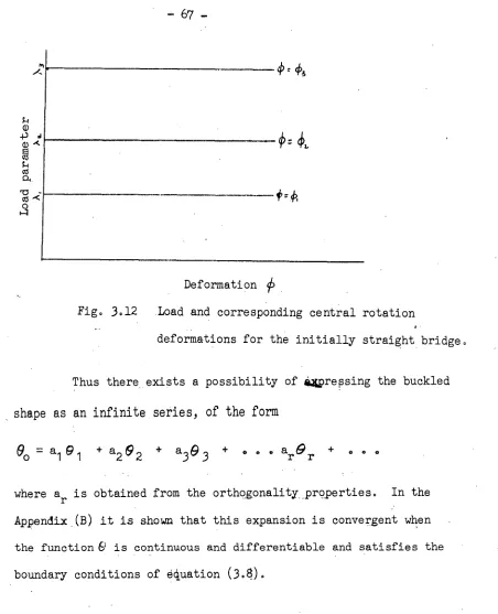
stability of a pin-ended column. This review is used as an introduction to the use of a characteristic geometric describing shape in the study of structures liable to buckling instability. It is shown that for many years engineers have recognized the values °fusing an infinite Fourier sine series (derived from the different: equation

describing the behaviour of the pin-ended column) to describe an arbitrary deformed shape. This method is useful when the structural behaviour can be represented by those differential equations for which sine functions are a solution. However, the existence of other

to generalize the well known plot, first developed by Sir Richard Southwell (Ref. 3)0 This generalization provides a link between the initial and final shape of the structure with the loadings on the structure for a large

range of structures liable to instability. With this sound analytical basis, reinforced with measurements taken on actual structures, the Southwell Plot becomes a more valuable experimental and design tool. The author believes that this generalization is original.

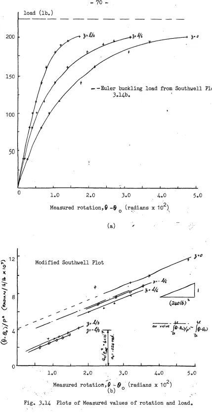
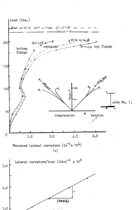
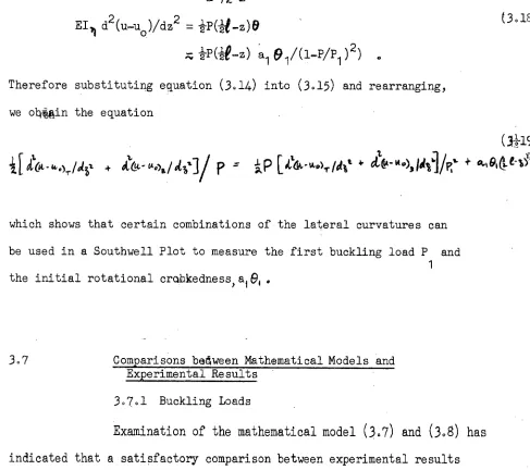
Chapter Three is the first of three chapters which are concerned with the design of a through bridge. In this chapter the measurements

taken on a simplified light through bridge are outlined. It is found

that the model through bridge is liable to lateral and torsional

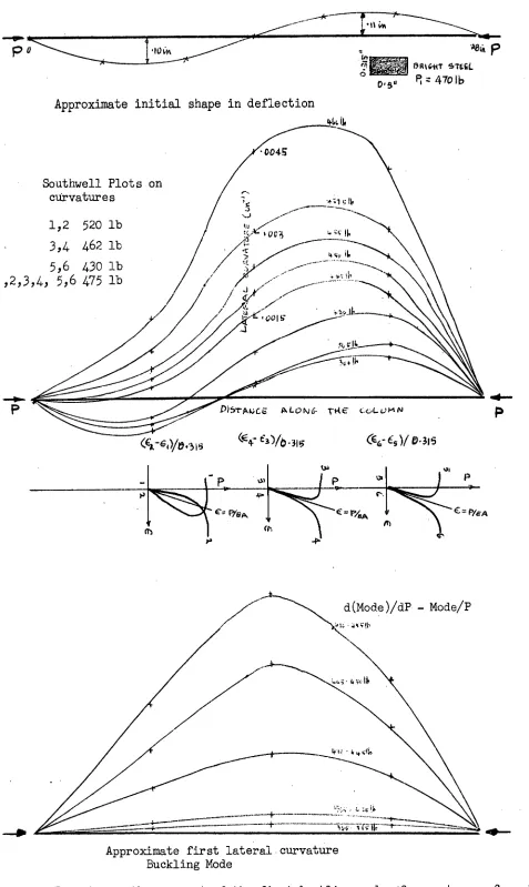
instability. A new mathematical model is developed to describe these lateral and torsional movements, and upper and lower bound solutions to the first buckling load are found. These loads and the corresponding buckling modes are shown to be a reasonable approximation to the measured results. Other original contributions outlined in the chapter include

Southwell Plots on

rotations and on strains suitable for use with the

new mathematical model for the bridge, a method for separating the first buckling mode from the measurements of the total deformed shape, and a method for finding lower bound solutions in some structural problems.

In Chapter Four the effects of minor additions to the laboratory and mathematical model are investigated. The first effect described is that resulting from the inclusion of web stiffeners inthelnodel through bridge. The inclusion of web stiffeners is shown to change only slightly the nature of the deformed shape, and to increase by only a small amount the buckling load. The second effect described is that of loadings

applied at points other than through the centroid of the I beam. It is shown that lateral and torsional loadings applied to the bridge can

In Chapter Five the author discusses the design of real through bridges. An examination of existing code recommendations indicates that there exists a large difference between these recbmmendations

and the measurements I,aken on the light through bridge (outlined in

Chapter Three). To gain a greater appreciation of these differences,

five additional model steel bridges are tested in the elastic and elasto-plastic ranges of deformation. A good fit to these model test results is shown to be the mathematical model developed in Chapter Three and, as a result of the understanding gained from these model test results a process for use in the design of

light through bridges is established. This design process is

then checked by comparing these predictions with measurements

taken on a full-size structure. In the light of these tests, design recommendations for light and heavy through bridges are

In Chapter Five the new mathematical model developed in Chapter Three is consolidated, and the limits of this model are found in relation to existing mathematical models for heavy through bridges. Also in the chapter a simple approximation to the buckling load is found, and the concept and use of a line of first yield using simple patterns of the deformed shape

of the bridge is presented.

In Chapter Six the range and the power of the method of functional form is illustrated by presentation of a description of torsion, as this problem of torsion arises naturally in the discussion of the deformations of the twisted and bent through bridge. It is shown that present methods to describe torsion depend on analogies (physical and mathematical), and at best describe shear stresses in terms of the slope on a thin film

membrane, or in terms of the solution of a high order differential equation.

twisted member.

Coidamb

(Ref. 4) used this approach and obtained the good approximation for a twisted circular bar that "plane sections, perpendicular to the longitudinal axis of the bar, remain plane". This approximation is a poor estimate of the deformations of a rectangular bar, and improving approximations could not be found. Later analysis of the torsion problem has therefore tended towards a more rigorous mathematiCal treatment. Nevertheless, further consideration of the deformations of the twisted section leads to the first approximation that for small angles of twist all straight

lines originally parallel to the sides of the member remain straight

after the member has been twisted. The behaviour of many

twisted members with open and closed cross sections is investigated by using this basic approximation, and an original, complete, and simple

pidture

of torsion is developed.

The research presented in this thesis is part of a continuing project in structural analysis being carried out under the direction

of Professor A.R. Oliver in the Civil Engineering Department, at the University of Tasmania, Australia. The author has been involved in this research from March 1965 to September 1967, and has been studying under a scholarship provided by Imperial Chemical Industries of Australia and New Zealand.

The author has published a number of papers and discussions concerning the research outlined in this thesis. A list is included at the end of the thesis.

Professor A.R. Oliver, the Professor of Civil and Mechanical

Engineering at the University of Tasmania, and

Dr. M.S. Gregory, Reader in Civil and Mechanical Engineering

at the University of Tasmania, and supervisor of this research.

The author has also had help in the form of correspondence, or

discussion from the following persons:

Mr. J.P. Hill, Chief Engineer, Maring BOard of Devonport, Tasmania Dr. M. Lay, State Electricity Commission, Victoria,

Mr. G. Sved,

University of Adelaide. Dr. N. Trahair, University of Sydney.

Dr. C. O'Connor, University of Queensland, and Professor B. Johnston, University of Michigan, U.S.A.

I hereby declare that, except as stated herein, this thesis contains no material which has been accepted for the award of any other degree or diploma in any University, and that, to the

CHAPTER ONE

MEASURING GEOMETRY TO OBTAIN SIMPLE MATHEMATICAL MODELS

101 Introduction

The formulation of any engineering problem is very conveniently

thought of as containing

accy

three phases, (Refs.

5

and 6), These

ares the real problem, the physical models, and the mathematical models. The real problem is initially a vague and undefined notion. It May be the "investigation, design, and construction of a bridge", while one of the physical models could be described as the bridge

structure itself ) or the simplification of it used for structural

design purposes. The bridge structure

may

have a certain type and

number of beams, columns and decking, and the physical model is often further defined and simplified in such a manner as to be more amenable to description. Any description of the behaviour of these physical models which depends on logical analysis is called a mathematical model. In engineering analysis the mathematical and physical models are gradually modified and used to formulate and describe the real problem and enable a reasonable mathematical model to be obtained.

All structural analysis is necessarily approximate, and to obtain a mathematical description a functional relationship must be used to connect some of the variables. A specific example is the stress-strain relationship used in structural analysis. It is rarely fruith4 for the structural analyst to question the nature of the mutual attraction of molecules or even to use the Newtonian functional description of the problem, that is that there are mutual forces of attraction between molecules which can be described approximately as varying in terms of the inverse of the square of th4 distance between the molecules. For most

structural analysts this description is far too specific and it is sufficient to try to describe the overall stress and

interpolation. Fortunately, the functional description of this relationship for some materials is sufficiently well described by

straight lines over part of the practical range of strains. Since all structural analysis is approximate, there exists a variety of ways in which the variables of the problem can be considered and manipulated. The method presented in this thesis

is one in which a pattern is_used to link the important deformations

of the problem. This pattern, obtained from detailed measurement of model structures is described in terms of an analytic function, or functional form. With this overall estimate of the deformations, the forces to sustain the prescribed shape are easily found.

This is one of the oldest approaches of engineering analysis and the most powerful methods of analysis of structures have been along these lines. However, the source of the power of the method is not generally recognized. To show that the source lies in the use of a functional form or pattern to describe the deformations of the

structure, a few historical estimates of the deformations of a

bent beam are outlined.

1.2 The Beginnings of Structural Analysis

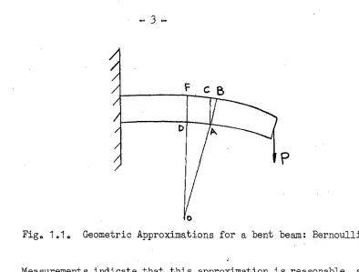
Structural analysis had its beginnings in the seventeenth century when mathematicians and geometricians like Mariotte and later Leibniz, Varignon and the Bernoulli brothers (Ref. 4) made approximations with regard to the displacements of bent bars. Jacob Bernoulli, when trying to calculate the deflections ofa loaded cantilever took the deflection curve as shown in Fig. 1.1.

[image:12.548.75.469.37.336.2]

Fig. 1.1. Geometric Approximations for a bent beam: Bernoulli.

Measurements indicate that this approximation is reasonable, as the cross section AB remains reasonably straight. However, we now know that a better approximation for the line of zero strain is obtained by assuming that the cross section rotates about some point inside the beam, the position of this point depending on the particular material and the way it deforms under load.

Bernoulli's approximations allowed advances in structural

analysis and the calculus was used to further the study, particularly the Euler column theory. A unified approach was made by Parent and later by Navier using the approximations that cross sections remained plane to describe the bending of plates and bars.

Later mathematicians developed more complicated models to describe the behaviour of structural elements, but they incorporated the smallest possible number of geometric approximations regarding the deformed shape. These developments have led to the mathematical approach involving stress function solutions, biharmonic solutions and high order differential equation solutions.

Improved mathematical models(using the mathematical approach) are obtained when a decrease is achieved in the number of

approximations needed to specify the geometrical deformations, or when further account is taken of the complexity of the functional dependence of stress and strain, or when further

The aim of a mathematical approach is then to make minimal assumptions or guesses of functional dependence, and to develop a complete description of a defined problem from a system of basic axioms, without the need for an appreciation of the deformations of the structure.

The mathematical approach is often useful in obtaining

numerical

solutions in particular cases, but because of their inherent generality, it can be remarked that

(a) often little understanding of geometric deformations, and load carrying meelanism of the problem is achieved, and hence methods of strengthening the structure are difficult

to visualize,

(b) a complete mathematical solution must frequently be obtained before useful information is available,

(c) allowance for second order geometric deformations is often not appreciated,

(d) as

regards teaching methods ) an engineering attitude is not

encouraged and a great deal of time is spent on merely illustrating a routine mathematical calculation.

As a means of overcoming these objections it is useful to look back in history and to glean a few ideas of how the advances and

simplifications in structural analysis have been made. When we do so we often find that these advances in analysis have been achieved by the use of approximate descriptions of displacements, and as a

result the mathematical complexity of the problem has been considerably

reduced.

Throughout this thesis it is shown that patterns or characteristics of the geometrical deformations of structures, (such as displacements and surface slopes)enable good descriptions for a range of structural problems. Analytical functions are used to describe these geometrical characteristics, and from these functions, strains are defined. Estimates for load

deformation relationships are used to define stresses and from an integration of these stress patterns the forces which must be applied

This inverse method has the advantages that the mathematics remains simple. At each stage of the computation the physical

significance of the geometrical approximations of functional

dependence is obtained very clearly, giving a deeper insight into

the effects of the geometrical deformations and the assumptions which have been made about them. This insight Tiables a good appreciation of the structural behaviour to be developed, and quick and reliable estimates of the effects of stiffening the structure 4e-ee-mErde., or of lightening if it is unnecessarily strong in some places, can be made.

1.3 Using Patterns in the geometric deformations to obtain simple Mathematical models

1.3.1 Measuring Devices.

In this chapter the use of geometric information obtained by moire techniques is discussed, particularly measurements showing the position of lines of constant displacement in the plane of the model

(Ref. 7) and the position of lines of constant slope on the surface of the model, (Ref. 8). Later in the thesis these ideas will be applied to measurements of an overall shape obtained from many point by point

measurements.

Overall detail of geometric deformations using the moire technique is a particularly suitable set of measurements for the -following reasons.

Geometrical effects are always separable from other considerations and a deformed shape can always be drawn without any consideration as to how this shape was obtained. Considerable information can thus be obtained before concepts of stress and statical action

are introduced, the reasoning being thus simpler and more

straightforward than that obtained by introducing stresses

too early. Variables of statics (force variables) are frequently not separable.

(b) Lines of constant slope and lines of constant displacement are

easy to obtain. The patterns suggested by these contour lines

are usually simple, and suggest the nature of the functional

form. As they are direct measurement of deformations they can then be used to establish a simple mathematical model. The order of complexity of the model is then determined by the approximations made of the deformed shape of the structure. (c) The shape of the moire fringes (or contours), can be used

to suggest structural behaviour which is common to various structural models. When the same functional form is a good fit to different size models, then the functional form is

the scaling function.

(d) The whole outlook is concentrated on the production of simple descriptions of the load and deformation behaviour, and is thus suited to an engineering approach. With this outlook, simple models, suitable to be incorporated in codes of experience or practice, are always kept in mind. In the following sections very simple structural problems are investigated as a means of showing that the measurements of the geometrical deformations of displacements and deflections can be used to obtain simple structural models. Theearly problems are

-.7 —

manipulations involved in the process. It is well known that

the shape of an element of a stretched or bent bar, chosen with sides

parallel to the edges Of the undeformed bar, is approximately the same

as the deformed bar. These siiple problems are described in terms of a geometric functional form. The simple model for a twisted thin rectangular strip that specifies that the shape of the element is the same as that of the deformed bar is then an easy extension.

1.3.2 A Simple Model for a Stretched Bar.

A rectangular bar is stretched longitudinally. This problem is obvious to the structural analyst; however this simple problem is useful to illustrate the basic ideas*

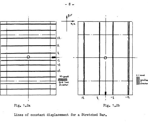
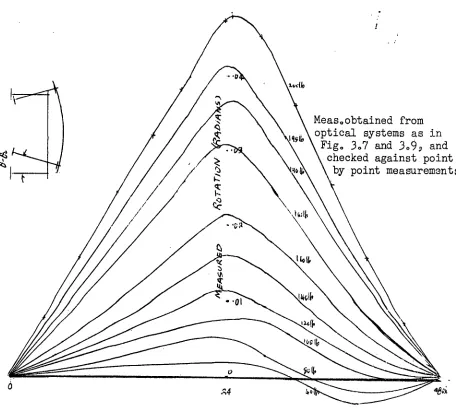
Measurements of lines of constant displacement (u 2 v) in the x 2 y directions are shown in Fig. 1.2a, and Fig. 1.2b 3 The

method used is the method developed in recent years -by Oliver, Jenkins L and Middleton at the University of Tasmania, and Outlined in Ref. 7. For completeness, the optical arrangement used to view the

interference pattern is shown in Fig. 1 0 3iland the interference fringes resulting from rotation 9 strains, and combined rotation and strain are shown in

Fig. 1.3b.

A good analytical description of the shape of these lines of constant displacement is given by the functions

u = y/a

and v = x/b 2

[image:17.549.39.528.39.442.2]

Fig. 1.2a Fig. 1.2b

0

MM. iricl

• Oliver-416A

tk.

0*. =

frtil kAL

Lines of constant displacement for a bent beam

Fig. 1.4a Irs1:1-,t1

Lines of constant displacement for a Stretched Bar.

1.3.3 A Simple Model for a Bent Beam.

Measurement of the surface deflections for the thin beam bent in a manner indicated in Fig. 1.4a indicate that the beam has single curvature in the longitudinal direction. Measurement of the lines of constant displacement u, v in the x, y directions Fig. 1.4a and 1.4b indicate that good approximations to the displacements are

U = a₁ x5r (hyperbolic) and v = b₁ x2 (parabolic).

(1.2)

collimator field

lens lens slit light

source

model reteren ce

screen

Fig. 1.3a Optical arrangement used to view interference patterns.

59 lines per inch

(a) ROTATION ALONE

(b) DIFFERENCE IN PITCH ALONE

(c) COMBINATION

OF ROTATION AND DIFFERENCE IN PITCH

51 lines per inch

-.9 -

.17

These estimates of U, v are particuldrly simple and as they have been expressed algebragially they may be said to express the functional dependence or the functional form of the displacements.

(-

The strains

E

_{x 3 y}

e

in the x, y directions respectively and the shear strain )( consistent with this function form, are

_u

xy

calculated from the approximations for small strain

e x = /ru/6 x

=

and = -ou,Aoy + -av/ax p

(1.3)

and are given by the equations

ex = ay

e = 0

_(1.4)

and oxy = (al + 2b1 )x,

For the bent beam, the stresses consistent with the

functional form (1.2) are

= (E/1- 2 ) al

y

0**1 = (E/1-12) al y (1.5)

'try.

= G(al + 2b 1 )x •

The forces necessary to sustain equilibrium are obtained by integration of these stress patterns and are given by the well known equations (using unit width of beam)

Axial load:

Vertical shear:

Bending Moment:

Px = (E/1-i2 )a1 y dy = 0 .41

Py = + 2b1 )x dy = 0

M = c(E/l -i2 )a1 y2 dy

the complete beam

- 10 -

where

= (E/1- 2 )a1 I 1 I = y2 dy.

-4.ot

If no total shear, P is applied, the relationship between constants a

1 and 2b1 can be found. Then, P = 0 gives a

l = -2b1 • (1 7)

The equation (1.7),when substituted into the last equation of (1.4) ) indicates that with the guessed functional form and the specification of no total shear we arrive at the obvious statement that the model is one for which no shear strains are present.

To sustain this deformed shape, a constant bending moment M given by the equation

M = (E/1 4) al I y (1.8)

must be applied to the beam, and the displacements of the section will be

u = (M/EI) (1 - 2 )XY

and

v

_{= -4(M/EI)(1-)2 ) x2}

(1.9)

It can

be seen from Fig. 1.4(A) and equation (1.2) that the

specification defines that plane sections perpendicular to the longitudinal axis before deformation remain plane and perpendicular to the longitudinal axis after deformation, and thus the shape of a small element chosen with sides parallel to the beam deforms in a

similar shape to that of the whole beam (Fig. 1.5), as Bernoulli assumed.

Dkria,b i4r3k44., 1==ast ri 11 d foie

Fig. 1.6b 1.3.4 A Simple Model for a Twisted Strip.

Measurement of the surface slope of a -twisted strip was carried • out by using the Ligtenberg moire technique (Ref. 8). This technique is simple and inexpensive to use. A brief summary of the technique is given in section 3.2. The measurements indicate that lines of

constant slope in the x, z directions can be delcribed approximately

by

a series

of

equally

spaced straight

lines, as shown in

Fig. 1.6..

Thus a good approximation to this surface shape is obtained by examining the form of .the vertical deformation w in the direction of the y axis, and is given by the equations

"bw/ax = kz, and 1!Jhz = kz

Fig. 1.6a

—1

kria,=u-mk

1101:41

hoe cliteotwet

Lines of constant slope on the surface of a twisted strip

Integration of equation (1.10) and choice of axes in the centre of the strip leads to the specification of the functional form defining the deflection of the surface as

— 12 —

, that is an anticlastic surface, with zero values for the curvatures

i

w/bx2 and 212w/z2 in directions perpendicular and parallel to the axes. However, rotation of axes by 450 to xl 1 z i gives the deflection as

/k(4 —

and the curvatures of "w/a4 and iw/az2

1 as equal in magnitude

but opposite in sign. As the investigation of the effect of transforming the axes is carried out on the mddel, or with the model deformations in mind, a better appreciation of the geometrical deformation is obtained.

Measurement of the surface displacements in the x z plane on the top and bottom surfaces of the strip by the method of Ref. (7) indicates that both these surfaces are in approximately pure shear but with

opposite sense. A slight inclination of the v lines indicates that a small amount of longitudinal strain is present, (Fig. 1.7a, 1.7b). In this first model we take the lines to be straight and parallel, and thus not consider the shortening of the member.

Fig. 1.7a Fig. 1.7b

/

LIBRARY

— 13 —

The functional form suggested by the lines of constant displacement

is

U = CZ

V = CX

and the only strains on the surface of the strip in the x, z plane are shear strains )1 given by equation (1.13) that is

u xz

(1.13)

The approximation that, straight lines .originally perpendicular

to the wide flat surface p of the strip through the thickness remain straights after deformation, indicates an element shape as shown in Fig. 1.$.

As all lines parallel and perpendicular to the sides of the strip have again remained straight after the twisting, our experience with examples 1.3.2 and

1.3.3

suggests that we try the estimate that the shapeof the element in Fig. 1.8 is similar to the shape of the strip ..' This estimate of the shape of the strip specifies the internal displacements. Each plane originally perpendicular or parallel to the longitudinal line of the strip warps into an anticlastic surface, (Fig. 1.9).

F = Mxy/b = Myz/

0

(1.15)

either F system or M system Fig. 1.10

— 14 -

The rotations da and d0 of one element relative to an xy yz

adjacent element or one warped cross section perpendicular and one warped cross section parallel to the longitudinal axis, relative to another

warped cross section is found from the element shape in Fig. 1.8. These rotations are given by

d9 xy 8 dz/it $

and dg yz =11 s dx/it )

and the geometric deformations are completely specified.

The only stresses needed to sustain the shape of this deformed

element are shear stresses, which can be specified bylr = G W • The

total forces required to sustain the guessed shape are two sets of twsiting moments M , M as shown in Fig. 1.10. Integration of

NY Yz

the stress patterns indicates that the magnitudes of these

twisting

moments are

M

xy

_{= [*b -t -2}

5

t] G[t

3

_b/6](d9,

y

/dz),

( 1 .14)

and Myz

= t] =

G [t 3i/63 (dOxy/dz) .

These twisting moments are statically equivalent to a balanced point load system, as the twisting moments per unit: length Mxy/b and M

yz dare equal. The applied force F, is given by the equation

— 15 —

Thus ., we obtain the well known relationship linking the end torque Fb with the twist of any element of the section,

Fb = [t 3b/31 (d9v/dz). (1016)

In Chapter Six, this simple model is extended to include the tapering off effects of shear strains at the corners,to describe the geometrical deformations of any rectangular bar

that has been twisted ) and to include the shortening effects

of twisted membersa

It can be seen that the examples chosen are particularly simple, but are basic. Examples, using the twisted strip as the basic element) are now considered to illustrate the power

and usefulness of simplg functional descriptions of the geometric

deformations.

1030,5 A Simple Model for a Twisted Member Built up. from Flat Strips.

Measurement of the' surface shape of an angle section

twisted by applying four balanced forces on one leg of the angle, indicate that the surfaces deform into shapes which are approximately anticlastic *. The angle between the legs in the plane of the cross section is almost preserved. .A simple model to describe this behaviour can be obtained as follows.

- 16 -

A cut is made in the joining corner as shown in Fig. 1.11, and the surface shape measured as before. It is found that each of the sides still deforms into a simple anticlastic surface, but that the angle between the legs increases slowly, as the slot length is increased.

The results summarized in Fig. 1.12 indicate that a proportion of the moment applied on one leg is transferred to the other leg within a very small region of width, approximately ten times the thickness of the

strip. Away from this region a good approximation is to consider the two strips as acted upon by separate sets of forces,the size of the forces

being in direct proportion to the width of the leg. The end torque

twist relationship is thus

Fb 4500] (delv/dz) • (1.17)

1.3.6 A

Simple Model for a Twisted Stiffener in a Twisted I Beam.

Repeating the tests of section 1.3.5 but using an I beam as the built up section,indicates that a similar model can be used, as all

surfaces on the I beam again deform in a manner which can be described

adequately by the simple anticlastic surface.

When a light transverse stiffener is placed between the flanges, as shown in Fig. 1.13, and the I beam twisted, it is found that the

I beam again deforms in approximately an Snticlastic manner. Measurement of the surface shape of the stiffener also indicates that the deformed shape of the stiffener can be described adequately by a simple

,•1 tU • G. ley

+10,ci4l■essi em% • GOY

Fovtes P Pi, a

0.4 cog 0°

Ca

— 17 —

•ow le.ok O. •„,embe,

Fig. 1011 Forces Applied to the

angle section.

Fig. 112, Plot of twist and slit length

light end stiffener

Fig. 1.13. Forces applied to I beam - stiffener arrangement

f

ES=

KAI,

Fig..1.14 Forces necessary to sustain the stiffener as an anticlasti.c surface

— 18 —

Application of the bimoment to the end of an I beam twists the entire I beam and bends the flanges of the I'beam. * When length

t

of the I beam is short and the width of the flanges b is largei a simple model describing the behaviour is obtained by application of the bimoment to an I beam built from three flat strips, and joined only at the corners Of the flange (Fig. 1.14).

Measurement of the surface shape indicates that a reasonable approximation is again the anticlastic surface, with no cross sectional distortion. The forces 111cessary to sustain the anticlastic shape are shown in Fig. 1.15, and are statically equivalent to the bimoment.

Thus, the applied bimoment B and the twist of the I beam can be related by the equation

B K h b = G[t

3

b/3]

,

e (deridz) . (1.18)

A description of the effect of the stiffener can be found using this model. The stiffener slightly reduces the magnitude of the twist, but the overall characteristics of the deformed shape (that is the

shape can still be described in terms of anticlastic surfaces) are not altered. The end torque twist relationship for

the I beam and

stiffener is given by the equation

Fb = GJ/[1—t.jSTIFF° GJ)] d9,/dz.

- (1.19)

— 19 —

1.4 General

Comments.

In the very simple models discussed it has been shown that the

determination of scaling factors is inherent in the choice of the

geometric functional form used to describe the geometrical deformations. Thus the problem of scaling, that is of relating the behaviour of the small scale model to the behaviour of the full size structure reduces to the problem of choosing a satisfactory functional form. If, when a particular model is studied closely, doubt arises as to whether the geometric deformations measured are a property of that particular size of model or of that type of structure, the problem can be overcome easily by testing several models of different sizes.

The choice of a functional form is especially suitable in any analysis when linear, quadratic or sinusoidal dependence relationships can be established, and when searching for a describing characteristic it is important to measure variables which highlight these types of dependence.

Throughout the history of engineering analysis, functional forms have often been used to describe characteristic features of similar problems. For example, empirical rules have long been used in

engineering with considerable success but have usually been restricted to describing a final state, rather than a form or observable 7lattern that is obvious in the early stages of the description of a problem. However a notable example in structural analysis of using a functional form to describe geometric deformations is the "plane sections remain plane" rule for the bending of beams in metallic or concrete

- 20 -

to describe geometric displacements has been proposed by J.K. Wilkins (Ref. 10) who uses it as a means of describing and designing for the behaviour of the concrete or bitumen waterproofing layer on the upstream face of decked rock fill dams.

Energy methods of structural analysis are another important use of guessed and measured functional forms of the deformations of the structure. The energy process based on potential energy is merely an averaging device where certain averages of some of the equations of statics are satisfied and are used to obtain good estimates of the

variables within the functional form. However, in much modern analysis the functional form chosen is usually an infinite series of sinusoidal waves. Unfortunately, in many problems one or two sine waves are not a good functional description of the deformations, and thus when the infinite series (with no single term being dominant) is used, an

appreciation of the deformations is often lost within the mathematical manipulation.

*

Throughout this thesis a deliberate effort is made to look for and describe characteristic shapes which define the deformed structure. The method is used first to gain an understanding of the problem of

buckling instability, and a detailed study is made to show that the existence of characteristic shapes can be used to describe this

- 21 - CHAPTER TWO

AN OUTLINE OF THE INSTABILITY PROBLEM.

2.1 Introduction

The cabestion "Is an engineering structure Is stable under

the action of the applied loads?" is a question which is easily asked. However, to provide a satisfactory answer, a good appreciation of the possible deformations of the structure is necessary, as the stability of a structure is some measure of how the deformations of the structure increase as the loading of the structure is increased.

All structures deform under the action of loads, and the

actual form of the deformation is often the important criterion. Consider, for example, the determination of the stability of a dam. The dam is considered unsatisfactory, or unstable, if the loadings on the dam cause the dam to lift or to overturh. The problem still remains of how much to alter the dam design so that the new shape is stable, and engineers sometimes design the dam so that the joint between the dam and the foundation is everywhere in compression

over the complete range of design loads. However, this is not always a satisfactory criterion of stability, as we find when we try to estimate the stability of an axially-loaded slender column. When the column is loaded, points on the column deform in a direction approximately perpendicular to the applied load. One measure of the stability of this structure is by what amount the structure deforms when the load is increased.

This Chapter will be mainly concerned with the problem of the stability of fritme and plate structures. In these cases,

instability may be considered to be the phenomenon of the occurrence of large relative changes in the geometric deformations of the

- 22 -

The Chapter is designed to re-inforce and add to the existing work on structural stability as outlined by Euler (Ref, 4), Southwell (Ref. 3), Gregory (Ref. 11 and 12) Ariaratnam, (Ref. 13), Crandall (Ref. 1 4),

Courant and Hilbert (Ref. 15), and Miklin (Ref. 16). Particular attention is focussed on the description and measurement of deformed shapes and of buckling loads and the Southwell Plot, first used by Southwell (Ref. 3) to estimate the first buckling load of a pin ended column, is generalized

for a range of mathematical models. Although the mathematical manipulations

used are well known by mathematicians, engineers have not taken advantage . of the power of the methods used, and the author claims originality for this generalization of the Southwell Plot.

As a first step in the discussion of structural instability,

the well known and simple model of an axially loaded column

is

considered. The description of the behaviour of the loaded column is similar to the approach developed by Gregory (Ref. 12) •to describe general buckling phenomena in terms of the simple example of rigid rods and lateral eprings. However, the column example has been chosen to emphasize that a continuous system can be thought of in the same manner

as a discrete system. Often it is easier to evaluate and find, properties

of the discrete system and then carry these properties over to the

continuum. Hence, the well known column

example is

outlined thoroughly

and the ideas obtained are then used to develop generalizations.

2.2 A Simple Model for the Axially Loaded Slender Column

The design of an axially-loaded slender column will be considered. The first step in this design process is to obtain a description of the deformations of the system. It is well known that

- 23 -

The simplest model chosen is shown in Fig. 2.1. This simple and well known model consists of two equal uniform rigid straight rods, joined by a spring which resists the jangle change between the rods. The rods are compressed by thrusts which remain axial, and the ends

of the rods are considered as pin-ended. This particular model

is such that all geometric deformations can be described by one

parameter, the central deflection of the rods.

Fig. 2.1. Rod and Single Spring Mechanism.

Examine the stability of the system when a small lateral perturbation y of the hinge is applied. The central lateral

deflection y is sufficient to describe the deformed system,

consisting of two straight lines and a central hinge. The change of angle

9

between the two straight lines at the hinge is, for small values of the lateral deflection

0 = 4y/i

(2.1)

The forces to sustain the deformed system are then found easily. Let us specify a linearly elastic rotational spring. The load deformation relationship is then a relationship(in this case called the spring constant k) between the change of angle at the hinge and the moment M developed by the hinge. The required relationship is

M = k

hinge deflection is undefined

d P= 414

- 24

The conditions for the system to be in statical equilibrium can then be found, as the moment M developed by the spring must be equal to the moment of the applied axial load P taken about the spring. Thus a we obtain the mathematical condition for statical equilibrium, namely,

M - py = 0, (20)

and using equation 2.2 1 we obtain an equation showing the relationship

between the deflection and the load, and

(44 ,

F)y = 0 . (2.4)

A

mathematical solution to equation (2.4) is obtained from

inspection: either y = 0, that is the column remains straight, or,

at

a buckling load P given by

P = 41cte

the deflection of the hinge is undefined (Fig. 2.2). Nevertheless the form of the deflected shape is defined and consists of the two straight lines with a central hinge (Fig. 2.2). This form is called the buckling mode.

load

— 4k/g deflection of the hinge is undefined, y = 0 but the shape of the

mechanism is defined

deflection of the hinge

deformed shape • at P = 414

Fig, 2.2 Behaviour of the Mathematical.Model

- 25 -

A

closer representation of the real problem is obtained by modifying the physical model shown in Fig. 2.1 to include the

following: initial crookedness of the column', an increasing number 0?

hinges, and allowance for second order geometric deformations,

non-linear load deformation relationships

and a closer specification

of the loading and boundary conditions. In the following sections, methods which include each of these effects in a large range of mathematical models are examined, and it is shown that a close representation of the behaviour of many real structures subject to instability is obtained.

2.3 Initial Crookedness in the Mathematical Model

The inclusion of initial crookedness in the mathematical model is a worthwhile and well known improvement and adds to the

understanding of the real problem. Suppose the initial lateral

deflection of the rods is yo , and the rods between the spring remain straight.

The geometrical estimate of the deformations is again determined by the central lateral deflection. The initial rotation of the hinge

Goe ,

is given by the equation

9

0

=

₄

wv,1

The load deformation relationship is dependant on the change of angle between the two straight rods, and is

(2.5)

= (414)(Y - Yo) *

y = 0.025 ° 0.05

001

—26.

('

4

/2)(y y0) P Y =

(2.6)

The deflection of the hinge is obtained in terms of the applied load and initial deflection, and we have

(2.7) = Yo/(1— Pir4k) 0

This mathematical model (equation 2.7) indicates a steadily increasing deflection of the hinge for loads ranging from zero to close to the load given by

P1 = 414 a

This load P

1 , called a buckling load in the previous model, is a good describing feature of the two physical models. In Fig. 2.3, a range of values of initial crookedness is plotted and it is seen that for very

small initial crookedness values the two mathematical models expressed by equations (2.4) and (2.7) are similar.

load

P = 414

CO 0.5 1.0

Deflection of the Hinge

Fig. 2.3. Equation 2.7, with a range of initial crookedness values.

= (_/o.4

and

C

Z

t

2

1'40

-

_C.Le

and

(-1.5k/t)y₁ that is in matrix notation

+ (3k4-1) )y2 o 9

— 27 —

2.4 An Increase in the Number of Hinges.

2.4.1 Two Hinges.

A closer representation of the behaviour of the column is obtained by increasing the number of hinges. When the number of

hinges and springs is increased by one, as shown in Fig. 2.4, the

geometrical relations between the angles

9

and

9

and the corresponding

2

deflections, yi and yz 1 (for small lateral deflections) are

(2.8)

Fig. 2.4 Rod and Two Springs.

The moments sustained by the linear elastic springs are

and

M

2 = kg2

The conditions for statical equilibrium are found by considering the equilibrium of the two rods separately, that is

M1 - PY1 = ° 9

and

M2 — PY2 = *

Combining equations (2.8), (2.9) and (2.10) gives the system of linear simultaneous equations that must be satisfied if the system is to remain in statical equilibrium

(3k/2— P)yi — (105k/Cy2 = 0

(2.11)

(2.9)

load or simply

-

28

-

.3

1

4-

P -1.5k/yi

°

[1.51Ve 3kAt-P =

A ][y =

The solution of these two linear simultaneous equations is given either by the trivial solution that the hinges do not move, (y1 = yt= 0,)or

(34- p) 2

(105k/e)2 = 0 ₉ (2.14)

that is the determinant of [A] is zero. The two non trivial values of load which are solutions of equations (2.14) are either P, = 1.5ka or

Pi = 4.5

kLe ,

and the corresponding buckling modes can be determined from the lateral deflection ratios of the hinges, = ;and = -

(Fig. 2.5).

P =

_1.5k/

Deflection of a hinge

Fig. 2.5 Behaviour of the Mathematical Model 2.13.

2.4.2. Initial Crookedness and Two Hinges.

A method to describe the effects of initial crookedness may now be obtained by use of the buckling modes for the initially straight structure. When the initial crookedness consists only of initial lateral crookedness at the hinges, two variables are needed to specify the shape. A linear combination of the two buckling modes is used to describe this initial crookedness.

An initial crookedness of the form yip= 1.0 , 49= 0.5 is expressed as a linear combination of the buckling modes, and

,

Aitgasn't

Loom'

1 .

0 _[1.0

I

{ 1

.

01

0.5

1

a

1.0

a 2

—1.0

(2.15)

— 29 —

initial first buckling second buckling crookedness mode: symmetric mode:antisymmetric.

The constants a and a are found easily by multiplying by the 1 2

transpose of the column vectors

ii-o

t. 01 and 1-0 respectively.

Then [1

0

0 1

0

01 1.0 = a

l

[00 1061 100 + a2t.]:80 100

,„.6

2.16)

0.5 1.0

That is 1.5 = 2a, + 0 a l

or a = + 0.75. Similarly, a l.= 0.25.

The initial shape, in terms of the buckling modes, is therefore

1.01 1.0 1.01

0.5 11.0] -1.0

= _{0075 + 0.251} (2.17)

The separation of the initial crookedness into a combination of the buckling mode components is useful in the

solution of the mathematical model for the initially crooked

structure, as it indicates the way in which the structure deforms.

The mathematical model for the initially crooked structure consisting of thrbe straight rods and two hingeA ie obtained in a manner similar to the one hinge case. The initial rotations

9

_{go to} and 0 are linked to the initial deflections

and yzo by equation (2.8). The load deformation relationships are then

14

1 =

1

091 —ai d

= (44)(Y1 — Y10)

(2.18) and

M2 = (414)(Y2 — Y20) °

For the structure to be in statical equilibrium, the moment

resisted by the springs must balance the applied moments (equation 2.10). On substitution of equation (2.18) into (2.10) we obtain the equations

-.30 -

310,- P -1.5k/ZIyf - 3k/j. -1 14

°5 Y11 314 - y21 -1.5ka 1a 3,

20 .

(

2

01

9

)

With values for the initial lateral crookedness of the hinge s(y lo and y20) as 100 and 0.5,, equation (2.19) becomes

P -1.51y1

[34

-1.511.0] -1.5k/11.01

= 0.75 +0.25

1.54 -P y2 -1054 - 1.0 31cLi 1.0

The right hand side of equation (2.20) is simplified by using the two solutions of equation (2.12), which are

[-

34 .

-1.5k/1

[1.

0

1 =

1.5k/t

L.0]

-1.5ka 3ka. ' 1.0] 1.0

[3

kte.

-1.5k11.0] =

4.5

k/e

and

{1

.0

The left hand side of equation (2.21) is simplified by separating the final shape into a linear combination of the buckling modes, and

1. Y2

1 [_1.01 + b2

[ Y11

= b 1.0

[-1.0 1.0

Then; from err..-a".1 , (2.20), (2.21) and (2.22) we have the equation

+ [1.0

1.0

[1.0 I

VW* _1.5kze 3ka -100

b

1

[ 3kAt- P -1.5k1[1.0 1.0

..1.5k/€ 34-p

_ P -1.511.0] [

34 4

b2 _{• -1.5k/2}

314 -P which simplifies to

P) 1

]

1.0

l.01.

1 0 .

0,75(1.5k/2) 0 . 25(4.54) 0.75(1.5ka) (2.21) (2.22) (2.23) (2024)

b₂ (4.5k/I- p)

{

1.01 0.25(4.5k4) 1.0

-1.

0i

61.01,

Equating terms with the same buckling mode, we obtain the values of the•

two buckling modes, and

1 =0.75 (1.5k/e)/(1.54-P) (2.25)

and b₂ = 0025 (4.5k4)/(4.54- P).

- 31 -

buckling modes of the structures, and

0075/(1-Pi/105k) 1.0 + 0.25/(1- 14/4.5k) 1.0

(2.26)

Y2 1.0 -1.0 •

final deflections first buckling mode second buckling mode of the hinges co-ordinates of the co-ordinates of the

hinges hinges

The predicted behaviour is shown in Fig. 2.6. For loads less than the first buckling load, the deflection always increases with load, and has the same sign as the first mode initial crookedness. However, because of its discontinuous nature the buckled shape is still not an adequate description of the shape of the deflected column, and thus

it is necessary to increase the number of hinges

)

deflection

Fig. 2.6. A Graph of Axial Load and hinge deflection, for the initially crooked column.

2.4.3 A Farther, increase in the Number of Hinges.

The number of hinges can be increased indefinitely. In the continuum, the change of angle per unit length along the bar is approximated by the lateral curvature (d 2y/dx2 ) of the bar, and the moment rotational deformation relationship is related by the flexural

-32-

El d2y/dx2 +

P

y = 0 . (2027)

The behaviour of the mathematical model (2.27) near the end of the bar is obtained separately. To be of value these descriptions should be at the same level of approximation as the differential equation itself. For the differential equation model of the slender column, the boundary conditions are *

x = 0 and y = O. (2.28)

The solution of the differential equation (2.27) is

y = A sin- x /177ET +. B cos 4177EY (2.29)

and

with the boundary conditions (2.28), particular solutions are obtained.

Use of the boundary condition x = 0, y = 0 gives B = 0, and the .boundary condition x , y= 0 .gives

0 = A

singl—P7E

9 _(2.30)

that is either A = 0, and the continuous system remains straight, or the

deformations of the system are sustained by a load given by the equation

0

= sin

/1771

(2.31)

i.e. p = n272E142 . _{where n = 0, 1, 2, 3,}

_{4, . 0 .}

These discrete values of load are called eigen values, latent rqots, buckling loads or, as this particular family was found by Euler, Euler

buckling loads. To each buckling load there corresponds a buckling mode (which is found by substituting into the equation) and the eigen functions, latent vectors, or buckling mode are

buckling mode y: sinTrx/e sin

21iv2

sin

31* )V.e

buckling load P:

72Eviz

2

9 41PEI/t2 9-11EIX,e2 9 o o

-33—

2.4.4 Describing Initial Crookedness in the Continuum..

A description of the effects of an initial crookedness of the continuous column can be obtained by using ideas obtained from the systems which had only a finite number of variables. For example,

including the initial crookedness in the mathematical model for the

continuous column, we obtain the differential equation

EId2(y— y o )/dx2 +

P

y = O. (2.32) Again the aim is to describe the initially crooked shape as a linear combination of the buckling modes. Southwell (Ref. 3) first developed this method for the pin ended column, but for completeness

and to outline the method the solution is given below.

The existence of a unique linear expansion for the initial crookedness yo , is used, that is the initial crookedness is expressed as an infinite series expansion

ao y

o = n sin nrx/t (2.33)

,A=1

This exapnsion is the well known Fourier Series and the justification and properties have been investigated by many authors

(see for eianTle Miklin, Ref. 16).

The coefficients a w are found by multiplying both sides of equation (2.33) by the Ta buckling mode, and integrating over the length of the structure. Then

t 60

f

1

Y

o sin mlix/t dx = Ian isin nWX/e sin mir x4 dx . (2.34)

0 rk71 0

As before, the product of two different buckling modes is zero. This property is called the orthogonal property of the buckling modes and enables a simplification of equation (2.34). The value of a is given by the ratio

a

m = ify sin miTxa dx o fn dx

—34—

The final shape, y and the initial shape ya are expressed as linear combinations of the buckling modes,

00 y =

n sin n7x/e (2.36)

n'■=1

and

00

Yo = an sin niTx/e e

(2.37)

Equation (2.32) is simplified using equations (2.36) and (2.37) and becomes

00 co

EI(bn-an )d2 (sin nwx4)/dx 2 + Pbn sin nrx/e = 0 But as

El d2 ( sin nirpa)/dx 2 + n2 ir2EI/t 2 sin nr)(49e = 0

then

22

_{(bn an)sin nr4 + Pbn sin mile= 0.}

N=I 117-1

(2.38)

(2.3

9)

(2.40)

Equating terms with the same buckling modes, we have on simplification

bn = an/(1-P/Pn ) 9 where Pn = n2 ir2EI/i2 (2.41)

The final shape, given in terms of an infinite series expansion of the

buckling modes of the initially straight system, is

y = [a1 )(1-P/P1 )] sinvrx/t + [an/(1-P/P2 )] sin 2Incje+

2.5 Comparisons between Experimental Readings and the

(2.42)

Mathematical Model

The mathematical model is now at the stage where comparisons can be made with experimental measurements. Southwell (Ref. 3) has presented a reliable method of comparison subject to the restrictions

P, load in .pounds

45511% pfo+e iine, in./Levi:wick p=

o oa4 •

4-1

3000

2000

1000 P

tc0

P= 0.8 x 10-5

P

crit= 2800 lb P

1 = 2800 lb a

o = 0.023

— 35 —

y _{[8.1 /(1- P/Pi ] sinlrx/e} (2.43)

The mathematical model is easily manipulated into a form from which the measured results can be compared. The form is

(y-a1 )sin/x/.94 =ey-al)sinTrx46#1 +(al sinnx/WP/ 9 (2.44)

that is the mathematical model indicates that a plot of the ratio of the

measured deflection to applied load against the measured deflection is a straight line. The slope of this line is equal to the reciprocal of the first buckling load, with the intercept on the load axis determined by the initial crookedness and the first buckling load.

Experimental readings of the load P and of the change in

deflection (y - yo ) at the centre of the column are found to be approximately hyperbolic. (Fig. 2.7). A horizontal asymptote to the hyperbola, that is

P = P Olt

is found from the reciprocal of the slope of the line of best fit to the Southwell Plot of the ratio of measured deflections to load against measured deflection (Fig. 2.8). The value of the horizontal asymptote P oo. found by this device is then used as a measure of P

I ' the first buckling load of the structure. The experimental results do not in general give a linear Southwell Plot, and hence a constant value for the horizontal asymptote P un t is not obtained, but often the deviations from a straight line are sufficiently small to enable a correlation to be made between experimental results and the mathematical models. A few of these .clOrrelations are now outlined.

10 measured deflection/load x 105

0.1

central deflection (in)

Fig. 2.7 Experimental readings of the central deflection of a pin ended column.

0.1 0.2

-

36

-

2.6 History of the use of the Southwell Plot.

Southwell (Ref.

3 )

was the first to observe that a plot of the load and corresponding mid point deflection of an axially loaded column was approximately hyperbolic in the neighbourhood of the smallest critical load of the mathematical model of the Euler column. He showed that the approximate position of the horizontal asymptote to this hyperbola could be obtained by a suitable transformation, namely plotting (y - yo )/P against y - yo where (3r 3r0 ) was the measured deflection and P the applied load, and drawing a line of best fit.

Southwell used the reciprocal of the slope of the line of best fit

as a Measure of the first critical load of the Euler mathematical model, He

justified this comparison by showing that when an arbitrary initial crooked-ness is included in the mathematical model for the Euler column as clAlined in section 2.4.4) the resulting model is a reasonable description of the experimental behaviour.

Donnell (Ref. 17) suggested that the Southwell Straight line plot

was a good measure of the first critical load in all cases of budkling, provided that appreciable second order stresses were not introduced, (such stresses occur when a developable surface buckles into a non developable surface) and assumed the validity of the Southwell Plot method in all cases where the corresponding differential equations were linear. However, it is sh6wn in the following sections that to obtain reliable correlations between experimental results and mathematical models, the mathematical

model must satisfy several other conditions besides linearity.

Dumont and Hill (Ref. 18) tested some aluminium alloy 1-section beams loaded about the major axis by a uniform bending moment. They found that the beams were subject to latek instability,and to obtain an estimate of the critical bending moment they plotted the ratio of the measured central rotation to the bending moment against the measured rotations. The reciprocal of the slope of the line of best fit to

— 37 —

showed that the reciprocal of the slope of the line of best fit of a

plot

of measured rotation to the square of the bending moment against the measured rotation gave a better indication of the square of the critical bending moment.

Galletly and Reynolds (Ref. 20) measured the elastic

circymferential strains and internal pressures for ring stiffened cylindrical shells subject to external hydrostatic pressure, and using Southwell's method were able to obtain the horizontal asymptote to the experimental readings. They were then able to

compare measured critical buckling loads with buckling loads

calculated from

a variety

of mathematical models.

Greogry (Ref. 21 and 22) showed that for structures bending in their plane and for triangular structure e bending and twisting out of their plane a correlation exists between the predicted first critical load and the asymptote obtained

from measured axial loads and curvatures by using the transformation as suggested by Southwell. Later, Ariaratnam (Ref. 13) justified mathematically the use of the Southwell Hot of measured

deflections, (and hence curvatures) and axial loads as a means of measuring critical loads in framed structures.

Thus, the Southwell Plot method has been of great benefit in the study of instability problems as reasonable estimates of initial crookedness and buckling loads have been obtained for a range of structures.

— 38 —

2.7.1 Extensions to the Southweil Plot

The ideas outlined in the orevious sections indicate

that

the Southwell Plot is a useful device for the comparison of some experimental results and some mathematical models. These ideas are based on the properties

--„

of the differential equation

El d2 (yi. y0)/dx2 + P _y.= 0. (2.45)

Many structures behave in a manner similar to that indicated by the experimental points shown in Fig. (2.8), but not all of these structures can be described adequately

by

the cne differential equation and set of boundary Conditions. A general test is proposed in the following section whereby any

mathematical

model, consistiniof linear differential equations and boundary conditions can be examine, see if a basis exists to compare experimental readings. After this basis has been established, firm design rules can be made with confidence.

Wien the analysis developed by Southwell is examined closely, it

is seen that the power of Southwell's analysis lies in the specification of the arbitrary initial crookedness. Southwell uses the terms of an infinite Fourier series to define the crookedness, as each of these Fourier terms is a solution of the mathematical model for the initially

straight structure. The description of an arbitrary initial crookedness for a different m4thematical model, as an infinite series, with each term a solution of this new mathematical model is now investigated.

2.7.2 Mathematical conditions sufficient to justify the Southwell Plot as a method of comparison of mathematical models and experimental results.

— 39 —

= a142 1 + a2 a33 * . a4) r r a (2.46)

Expansion (2.46) is valid if the following conditions are satisfied:

(a) a means exists to find the constants a l , a_s (b) the expansion is unique, that is the expansion is

linear independent,

(c) there exists an infinite number of solutions el, ' and (d) the expansion will converge as a, increased.

It is shown in the following section that when the

mathematical model satisfies the well known mathematical conditions of Rule No. 1, then the conditions (a) to (d) are satisfied and

hence the validity of the expansion (2G46) is established.

Rule No. 10 When the mathematical model for the initially undeformed structure can be expressed as a linear

differential equation of the form

L(4)) - A N(+) = 9

(2.47)

where L(e)? ) and N(4) are both self adjoint and positive definite differential operators and X is a load parameter, then the expansion 00 is valid.

Although the conditions required are readily available elsewhere (Ref. 16) for comple:teness an outline is now given of why the differential equation and boundary condition system satisfying Rule No. 1 satisfies the

properties (a) to (d).

Condition (a) is established when the operators L(11)) and N(4) are self adjoint. One definition of self adjointness is given in

i

[u L(v) - vL(u)] dz, and

ir

LUN(V)— vN(u)] dz are both zero.

4

- 40 -

(The points a, b define the positions of the boundaries.)

The implications of this condition can be seen when two separate so4tions of the differential equation (2.46) are examined, i.e.

L(r) _{X r N(cF r) = 0} (2.48)

and

L(44) - X s N(i) s) = 0 0 (2.49)

Multiply (2.48) by ( ) and (2.49) by ( ir ), subtract, and then integrate between the boundaries; the expressions become

4

f'

POtr)

-k.1(+8)] dz 14146 N(+r) N(+)] dz = 0 . (2.50) When L(1), and N() are both self adjoint, equation (2.50) can be • reduced to the equation

r 4 s)

N(ti)

r

) dz = 0

(2051)

k

t

r

when _)\s

(405

_{N(tr)dz = 0} (2.52)

Similarly, the relationship

L() dz = 0 , (2.53)

can be established. Equations (2.52) and (2.53) are called the

orthogonality relationships *. These relationships enable a separation of the variables a, , a l . For example, to evaluate the constants a ir , multiply equation (2.47) On both sides by N(4r) and integrate.

* A self adjoint differential equation is really another way of stating that the equation obeys the Maxwell Reciprocal Theorem - that is the cross product of generalized deformation U A at the point A multiplied by the generalized force L(U ) at the point B is equal to the cross product of the generalized deformation Viet the point B multiplied by the generalized force L(U ) at the point A. This statement may be expressed in the form

A