Coverage Performance Analysis of FeICIC Low Power Subframes

Subframes

.

White Rose Research Online URL for this paper:

http://eprints.whiterose.ac.uk/100514/

Version: Accepted Version

Article:

Hu, H., Weng, J. and Zhang, J. (2016) Coverage Performance Analysis of FeICIC Low

Power Subframes. IEEE Transactions on Wireless Communications, 15 (8). pp.

5603-5614. ISSN 1536-1276

https://doi.org/10.1109/TWC.2016.2562619

© 2016 IEEE. Personal use of this material is permitted. Permission from IEEE must be

obtained for all other users, including reprinting/ republishing this material for advertising or

promotional purposes, creating new collective works for resale or redistribution to servers

or lists, or reuse of any copyrighted components of this work in other works.

[email protected] https://eprints.whiterose.ac.uk/ Reuse

Unless indicated otherwise, fulltext items are protected by copyright with all rights reserved. The copyright exception in section 29 of the Copyright, Designs and Patents Act 1988 allows the making of a single copy solely for the purpose of non-commercial research or private study within the limits of fair dealing. The publisher or other rights-holder may allow further reproduction and re-use of this version - refer to the White Rose Research Online record for this item. Where records identify the publisher as the copyright holder, users can verify any specific terms of use on the publisher’s website.

Takedown

If you consider content in White Rose Research Online to be in breach of UK law, please notify us by

Coverage Performance Analysis of FeICIC Low

Power Subframes

Haonan Hu

, Jialai Weng

, Jie Zhang

1

_{School of Communication and Information Engineering, Chongqing University of Posts and}

Telecommunications, Chongqing, China

2

_{Dept. of Electronic and Electrical Engineering, The University of Sheffield, Sheffield, UK}

Email:

{

haonan.hu,jialai.weng,jie.zhang

}

@sheffield.ac.uk

Abstract—Although the Almost Blank Subframes (ABSF) pro-posed in heterogeneous cellular networks can enhance the per-formance of the Cell Range Expansion (CRE) User Equipments (UEs), it significantly degrades macro-cell total throughput. To address this problem, the Low Power Subframes (LPSF) are encouraged to be applied in macro-cell center region by the Further-enhanced Inter-cell Interference Coordination (FeICIC). However, the residual power of the LPSF which interferes the CRE UEs, and the proportion of the LPSF affect the downlink throughput together. To achieve a better rate coverage probabil-ity, appropriate LPSF power and proportion are required. In this paper, the analytical results of the overall Signal to Interference and Noise Ratio (SINR) coverage probability and the rate coverage probability are derived under the stochastic geometric framework. The optimal region bias ranges for maximizing the rate coverage probability are also analysed. The results show that the ABSF still outperform the LPSF in terms of rate with the optimal range expansion bias, but lead to a heavier burden on the back-haul of the pico-cell. However, with a static range expansion bias, the LPSF provide better rate coverage than the ABSF. Also, in a low range expansion scenario, the reduced power of the LPSF has negligible effect on the rate coverage with the optimal resource partitioning.

Index Terms—FeICIC, low power subframes, stochastic ge-ometry, Poisson point process, Signal-to-Interference-plus-Noise Ratio.

I. INTRODUCTION

With the proliferation of smart devices, downlink data traffic demand, for instance, video or game applications, becomes a growing concern in future cellular networks. Heterogeneous networks (HetNets), composed of traditional macro base sta-tions (BSs) and several different low transmitting power BSs are envisioned to be a powerful tool to meet the network traffic demand. The lower power BS leads to a smaller coverage area, but provides a better data throughput because of the closer serving distance [1]. However, the smaller coverage area, especially for open access mode pico-cells, results in fewer associated UEs. It is undesirable when macro-cells are already overloaded. In order to deal with this load imbalance, the CRE is adopted. It employs a cell range bias which extends coverage area of the pico-cell without increasing transmitter power [2]. Unfortunately, in this CRE region, the UEs become more vulnerable to interference from the underlaid macro BSs. To mitigate such interference, 3GPP Release10states that the ABSF, with no power transmitting on data channel at some coordinated time slots, should be leveraged in macro-cells.

However, the degraded performance of macro-cells caused by the ABSF, is brought into consideration in the literature recently. In 3GPP Release 11, the FeICIC is proposed. It advocates the allocation of the LPSF, instead of the ABSF, to macro-cell center region UEs at the coordinated time slots. It has been shown that the LPSF improves the the macro-cell total throughput [3].

A. Motivation and Related Works

Employing relatively high power LPSF will result in sig-nificant interference on the CRE UEs in spite of the macro-cell total throughput enhancement, which translates into lower SINR. In some worst cases, even basic modulations will be exacerbated. Furthermore, the desirable SINR does not necessary mean a qualified downlink throughput, which is also determined by the average allocated subframes directly. Therefore, analysing the overall SINR and rate coverage becomes critical.

However, only few works [4], [11], [12] analyse the per-formance of systems using the LPSF. Through hexagonal grid model simulation results from [4], [11], it is proved that the5th percentile and the median throughput improve. On the other hand, there is only one work [12] using stochastic geometry to study the total capacity and the5th percentile throughput of the FeICIC. Similar to [13], it allocates partitioning resources based on the presetting SINR value level. As a result, it is impractical to analyse the coverage performance based on the framework proposed in [12].

Despite the aforementioned research works, the study of the overall SINR and rate coverage probability of the FeICIC is missing in the literature, especially when the LPSF are employed. By employing the stochastic geometry, this work provides system design insights for the FeICIC scheme.

B. Contributions

In this work, we investigate the performance of the FeICIC when the LPSF are employed, under the stochastic geome-try framework. Initially, we propose a new user association method in the FeICIC by both the power reduction and the macro-cell center region factors. It extends the dominant interferer definition in [14]. We derive an analytical expression of the overall SINR and rate coverage probability in an integral form of the threshold, the power reduction factor, the path-loss exponents, the range expansion factor and the center region factor. An approximation of the Gauss hypergeometric function is applied to obtain numerical integration results. Based on the result, optimal values of the center region bias and the range expansion bias are obtained for maximizing the rate coverage probability. Furthermore, we propose an efficient single-iteration optimisation method to obtain these near optimal values. To our best knowledge, we are the first to discuss the optimal biases under the distance-based user association strategy. Eventually, we analyse the rate coverage performance with optimal biases and static range expansion bias respectively with comparison to the ABSF.

C. Organization

The rest of paper is organized as follows: Section II in-troduces the system model and the user association strategy. Section III presents the derivation of the analytical results and the optimal bias ranges. Section IV gives the simulation results before concluding in Section V.

II. SYSTEMMODEL

We consider a two-tier heterogeneous system consisting of macro-cells and pico-cells, modelled as two identically independent distribution (i.i.d) PPPs, denoted by M and P

with densityλmandλprespectively. They commonly share all

the frequency resources. The full transmitter power of macro BSs and pico BSs are denoted by Pm and Pp, respectively.

The macro-cells adopt the LPSF in center areas, with the power reduction factor ρ. Otherwise, the macro and pico BSs transmit at the fixed maximum power. With the assumption of Rayleigh fading, the received power of an arbitrary UE

MBS PBS

PBS

PBS P PBS up

pp pm

um up

pm um

um um

PBS PBS

p up up

pp pp

up

Macro-cell Center Region

Pico-cell Coverage Region Pico-cell

Expansion Region

Fig. 1. User association strategy

from a BS can be represented as P hr−α_{. The variable h}

denotes the fast transmitting attenuation on received signal power followingh∼exp(µ). The termr−α _{is the large scale}

path-loss, where r is the Euclidean distance and α is the path-loss exponent. Shadowing is ignored to avoid loss of tractability [6]. Moreover, every cell is assumed to employ a strict synchronization scheme [8] to coordinate interference between different resources. Under such an assumption, sub-frames with and without power reduction cause no interference to each other. In other words, the transmitting power of pro-tected subframes will not interfere the user using unpropro-tected subframes, and vice versa. If the LPSF among all macro BSs are not completely aligned, the center macro UEs and the edge pico UEs (both use the LPSF) will suffer severe interference from the neighbouring macro BSs. In particular when the pico BSs are deployed at the edge region, its users still suffer full power interference from the neighbouring macro BSs. Therefore, the misaligned model is not appropriate for the pico-cell deployment scenario. On the other hand, even if the LPSF are not fully aligned, we can still reach the results as in [12] by modelling with a fraction of the full power interference. However, it is obvious that the fully aligned model performs better than the misaligned model. The full power aggregate interference from other MBSs and PBSs are denoted as Im and Ip, respectively, and σ2 represents the

thermal noise. Then the common SINR expression can be represented as:

Φl=

ρlPlhr−lαl

ρl′Iml+Ipl+σ2

. (1)

as the LPSF in macro-cells are defined as the PSF, and the other subframes are defined as the USF. In such a case, the UEs are classified into four groups: protected subframe macro-cell UEs, unprotected subframe macro-macro-cell UEs, protected subframe Pico-cell UEs and unprotected subframe pico-cell UEs. We use the index l ∈L={pm, um, pp, up} to denote the four corresponding UE groups. Fig. 1 illustrates the four UE groups and their relationships to the macro-cell and the pico-cell. As shown in Fig. 1, closer center region associated UEs adopt the PSF in macro-cells to mitigate interference from other BSs. In contrast, PSF in pico-cells are allocated to the CRE UEs, who receive less signal power from the serving BS. The other UEs will be allocated with the USF, i.e., the pico-cell coverage region.

Then the SINR expressions for the four UE groups can be written as:

Φpm= ρPmhr −αm m

ρIm\{0}+Ip+σ2

, Φum= Pmhr −αm m

Im\{0}+Ip+σ2

,

Φpp=

Pphr−pαp

ρIm+Ip\{0}+σ2

, Φup=

Pphr−pαp

Im+Ip\{0}+σ2

,

(2) whereIs\{0} denotes the aggregate interference excluding the

serving BS. Since there is no cross-interference between the PSF and the USF, the value of ρl is determined as ρl = ρ

only if l =pm, and ρl′ =ρ if UE utilizes PSFs. Otherwise,

ρl=ρl′= 1.

We assume that the same group users share the same spec-trum resources in a round-robin manner [8]. Thus statistically the subframes can be considered to be allocated equally to the same group users, as the same group users have equal probability to obtain each subframe. By information exchange between the BSs and the UEs, the BSs know which UEs are allocated with USF and which UEs are allocated with PSF. Also we assume that the BSs know which subframes are configured as PSF and USF. Thus the scheduler runs round robin scheduling for PSF and USF users separately. Also, the BSs are assumed to follow a full buffer model, which always have backlogged data to transmit. In order to define the downlink throughput together with these SINR expressions, the resource partitioning factor (the proportion of the LPSF) is denoted as β. The probabilities of time-domain subframes configured as the PSF and the USF are β and (1 −β), respectively. Then the common throughput expression can be formulated as:

Rl=

βlW

Nl log2(1 + Φl), (3)

whereβlequalsβ and1−βwhen using the PSF and the USF

respectively. W is the spectrum bandwidth and Nlrepresents

the number of serving UEs, which will be discussed in Section III.

A. User Association Strategy

In this subsection we introduce a user association strategy, which defines the principle of the classification of a specific UE.

Throughout our analysis, we assume that a UE is placed at the origin position. It is a reasonable assumption because there is no difference in property observed either at a point of the PPP or at an arbitrary point, according to Slivnyak’s theorem [15]. Thus the UE association strategy is dependent on its nearest distances to the macro BSs and the pico BSs, denoted by rm and rp respectively. Thereby the user association

strategy is proposed for the two-tier network scenario. For the four user groups, we define the following association strategy based on the distances and range factors as:

Proposition 1. The UE’s associated BS and allocated

sub-frames follow the relationships between rm and rp as (4)

below, where kc, ke and kp are the macro-cell center region

factor, the pico-cell range expansion region factor and the pico-cell coverage region factor, respectively.

l=

    

   

pm, whenkcrm< rp

um, whenkerm< rp< kcrm

pp, when kprm< rp< kerm

up, when kprm> rp

(4)

The size of the macro-cell center region is completely depen-dent onkc. A largerkc results in a smaller size of the

macro-cell center region. Therefore, the PSF MUEs can be limited close to their associated macro BSs by a large enoughkc, even

if their nearest interfering pico BSs are distant. The value ofke

influences both the sizes of the pico-cell coverage region and the macro-cell coverage region. The value of kp determines

the coverage bound between the pico-cell coverage region and the range expansion region. In the pico-cell coverage region, the USF PUEs receive higher power from their associated pico BSs than any other macro BSs. Therefore, when a UE is deployed on this coverage region bound, its received power from the nearest macro BS Pm(kprb)−αm equals the

power from the associated pico BSPprb−αp, where rb is the

distance between the UE at the bound and its associated pico BS. If αm = αp = α, the value of kp is represented as

(Pp/Pm)1/α. Otherwise, kp has an approximation value of

(Pp/Pm)2/(αm+αp) [14].

In order to obtain the probability for each association case, the following lemma is proposed.

Lemma 1. In two i.i.d. PPPsΘi andΘj with densityλi and

λj, respectively, if the closest distances from an arbitrary point

to the PPPs are denoted asri and rj, then the probability of

ri> krj is given as:

Prob(ri> krj) =

λj

λj+k2λi

. (5)

Proof. See Appendix A.

The association probability for the USF MUEs and the PSF PUEs can be calculated by Prob(karm < rp < kbrm) =

8 9 10 11 12 13 14 15 0

0.05 0.1 0.15 0.2 0.25 0.3 0.35 0.4

α_m=α_p=3.0

B

m (dB)

User Association Probability

ABSF LPSF ρ=0.25 LPSF ρ=0.5 No ABSF or LPSF ρ=1

Fig. 2. User association probability of MUEs with various Bm values conditioned onλp= 3λm

the user group definition in (4), we have the probabilities for the four user groups as follows:

Prob(pm) = λm λm+kc2λp

, Prob(up) = k 2

eλp

λm+kp2λp

,

Prob(um) = λmλp(k 2

c −ke2)

(λm+k2cλp)(λm+ke2λp)

,

Prob(pp) = λmλP(k

e

2−kp2)

(λm+ke2λp)(λm+k2pλp)

.

(6)

In order to translate the variables kc andke into an

analo-gous form to kp, we definekc andke with the center region

bias Bm and range expansion biasBp as:

kc= (

BmPp

ρPm

)αm2+αp_{, k}

e= (

BpPp

Pm

)αm2+αp_{. (7)}

Therefore,Bp andBm can be written as

Bm=

ρPm

Pp

(kc) αm+αp

2 , B

p =

Pm

Pp

(ke) αm+αp

2 . ₍₈₎

In a special case, if ρ = 0, we define kc = ∞, where

its relationships to both ke and Bm are broken. In that case,

the PSFs are configured as the ABSF in the eICIC. The relationship of ρ, Bm, Prob(pm)and Prob(um)conditioned

on the same path-loss exponent is shown in Fig. 2, with the op-timal value ofkeobtained in Section III. The result illustrates

that the probability of the center region PSF MUEs improves (dotted curves) and that of the USF MUEs declines (solid curves with black dots) while the variable Bmincreases. The

corresponding markers are Monte Carlo simulation results.

B. Distribution of Serving BS Distance

After the users are associated to BSs based on their nearest distance to the BSs in different tiers, next we will discuss the probability distribution function of the serving BS distance.

We consider a typical user served by a BS in theith_{tier. The}

two-dimensional Euclidean distance from the BS is denoted as

ri and the nearest distance from the interferingjthtier BSs is

denoted as rj. Thus, we have the following results regarding

the distribution of the serving BS distance.

Lemma 2. The PDFfri(r)of serving BS distance conditioned

onrj> kri is

fri|rj>kri(r) = 2πr(λi+k2λj) exp −πr2(λi+k2λj).

(9)

Proof. Using Bayes’ rule, we have the probability ofri< R

with conditionrj > kri:

Prob(ri< R|rj > kri)=

Prob(ri< R, rj> kri)

Prob(rj > kri)

. (10)

The joint probability could be calculated as follows:

Prob(ri< R, rj> kri)

(a) =

Z R

0

Prob(rj> kri|ri=r)fri(r)dr

(b) = 2πλi

Z R

0

rexp(−λjπk2r2) exp(λiπr2)dr

= λi

λi+k2λj

1−exp(−πR2(λi+k2λj)),

(11)

where step (a) follows from the theorem of joint probability function and step (b) is derived from the probability of no point scattering in the region covered with radius kri in a

PPP. Combining with Lemma 1, we have the conditioned probability result as:

Prob(ri< R|rj> kri) = 1−exp(−πR2(λi+k2λj)). (12)

Then after taking partial derivative with respect to the variable

R, we obtain (9).

Using Lemma 2 and the user group definition (6), we have the PDFs of the serving distances in (13).

III. COVERAGEPERFORMANCEANALYSIS

This section is our main analysis part. We derive the integral form expression of the overall SINR and rate coverage per-formance with different path-loss exponents. Moreover, under the assumption of the same path-loss exponent, the expression of the rate coverage performance is derived. At the end of this section, the optimal bias values are discussed.

A. Overall SINR Coverage

We define the overall SINR coverage as the probability of SINR larger than a threshold, equivalent to the Complementary Cumulative Distribution Function (CCDF). The overall SINR coverage can be comprehended as the fraction of users who have better SINR than the threshold value. In our analysis, we assume the UEs and BSs are all static as a snapshot scene. Also, a UE can be allocated with either PSFs or USFs only. Then the overall SINR coverage probabilityPcov is given as

Pcov=X

l∈L

fpm(r) =2πr(λm+k2cλp) exp −πr2(λm+kc2λp)

fum(r) =2πr

(λm+kc2λp)(λm+k2eλp)

λp(kc2−k2e)

exp −πr2(λm+k2eλp)

−exp −πr2(λm+k2cλp)

fpp(r) =2πr

(λm+ke2λp)(λm+k2pλp)

λm(k2e−k2p)

exp −πr2(λm/k2e +λp)−exp −πr2(λm/k2p +λp)

fup(r) =2πr(λm/k2p +λp) exp −πr2(λm/kp2 +λp)

(13)

where Pcov(l) is the common expression of overall SINR

coverage of a typical UE. It can be further represented as follows:

Pcov(l) =Pcov(Φl> τ)

=E

Prob

ρlPlhr−αl

ρ′

lIMl+IPl+σ2

> τ|r

=

Z

R

EI

Prob

h > τ r

αl

ρlPl

(ρ′lIMl+IPl+σ2)

fl(r)dr

(a) =

Z

R

EI

exp

µτ r

αl

ρlPl(ρ ′

lIMl+IPl+σ2

fl(r)dr

=

Z

R

exp

µτ r

αl

ρlPl

σ2

EIM|l ·EIP|l·fl(r)dr,

(15) where step (a) is derived from the CDF of exponential dis-tribution h. The macro aggregate interference EIM|l and the

pico aggregate interference EIP|l can be further written as:

EIM|l=Eh,x

"

exp −µτ r αl_ρ′

l

ρlPl

X

m∈Ml

Pmhmxm−αl

!#

,

EIP|l=Eh,x

"

exp −µτ r αl_ρ′

l

ρlPl

X

n∈Pl

Pphnxn−αp

!#

.

(16) As the open access mode is employed, it is worth high-lightening that the nearest interfering distance has its lower limit. In order to calculate the aggregate interference, we have the following result concerning the interference from the ith

tier.

Lemma 3. The Laplace transform LIi(s) of the aggregate

interference from the ith_{tier is}

LIi(s) = exp

−πλi(

sPi

µ )

2

αi_C((kr)αi₍s

µ)

−1_{, α}

i)

, (17)

where function C(a, b)is

C(a, b)≈

   

  

A(b)−a2/b

1− 2a

b+ 2

, a <1

B(b)a2/b−1

1−(b−2)a −1

2b−2

, a≥1 . (18)

Proof. See Appendix B.

The functions A(b) and B(b) are defined as follows, and the function Γ(·)is the Gamma function.

A(b) =

Z ∞

0

(1 +xb/2)−1dx B(b) =−2Γ(2/b−1)

bΓ(2/b) (19)

If the interference and signal are both from the same tier, the minimum interfering distance is simplified as r withk = 1. For simplicity, we assume the thermal noise is approximately zero (σ∼0), which has negligible effect on the final results [5], referred as the interference limited network [16].

Equipped with Lemma 3, and E[exp(−sIi)] =LIi(s), we

have the following result regarding the overall SINR coverage of a typical UE in our network scenario as:

Theorem 1. The SINR coverage of a typical UE following the

user association strategy in (4) is given in (20)at the top of

next page.

Proof. Combining Lemma 3 with (15) and (16), we have the

result.

In (20), Pˆm = Pm/Pp and D(λ, α, t, τ) =

r2_λτ2

αC(τ−1, α). Moreover, the exponential part of the

integration in each equation is obtained by the Laplace transform of the aggregate interference from both tiers. Then we obtain the expectation value of coverage probability averaged on the serving distance r of the exponential part, which is the SINR coverage. With these results, we have the overall SINR coverage following (14). The closed-form result can be obtained when the macro-cells and pico-cells have the same path-loss exponent (αm=αp). Otherwise, we evaluate

the result numerically.

B. Rate Coverage

Similar to the overall SINR analysis, the common expres-sion of the rate coverage probability Prob(Rl> ω)is defined

as:

Prob(Rl> ω) =Prob

βlW

Nl

log2(1 + Φl)> ω

, (21)

whereω is the threshold of the downlink throughput andΦl

denotes the SINR of the user groupl. It can be comprehended as the average fraction of users achieving a target rate. In order to obtain the expectation of variableNl, we have the following

results with the assumption of an i.i.d PPP deployment of UEs with densityλu.

Lemma 4. The expectation of the UE number E(N) in a

Voronoi macro-cell isλu/λm.

Pcov(pm) =

Z ∞

0

h

exp−πD(λm, αm, r, τ) +λpr

2αm αp _{(τ( ˆP}

mρ)−1)

2

αp_C(k

cαprαp−αmρPˆmτ−1, αp)

i

fpm(r)dr

Pcov(um) =

Z ∞

0

h

exp−πD(λm, αm, r, τ) +λpr

2αm αp _(τPˆ

m −1

)αp2 _C(k

eαprαp−αmPˆmτ−1, αp)

i

fum(r)dr

Pcov(pp) =

Z ∞

0

h

exp−πD(λp, αp, r, τ) +λmr

2αp

αm_{(τ ρP}ˆ_m)αm2 _C(ke−αm_rαm−αp_{(τ ρP}ˆ_m)−1_{, αm)}

i

fpp(r)dr

Pcov(up) =

Z ∞

0

h

exp−πD(λp, αp, r, τ) +λmr

2αp

αm_(τPˆ_m)αm2 _C(kp−αm_rαm−αp_(τPˆ_m)−1_{, αm)}

i

fup(r)dr

(20)

Combining the Lemma 4 with user association probabilities in (6), then the four group average served UE numbers are as follows:

E(Npm) = λu

λm+k2cλp

, E(Nup) =

k2

pλpλu

λm2+kp2λmλp

,

E(Num) =

λuλp(k2c−ke2)

(λm+k2cλp)(λM+ke2λp)

,

E(Npp) =

λuλP(ke2−kp2)

(λm+ke2λp)(λM +k2pλp)

.

(22) Equipped with the expectaion results of UE numbers in (22), we have the following result regarding the rate coverage probability:

Theorem 2. The common expression of rate coverage

proba-bilityRcov(l)is

Rcov(l) =Pcov(l)|_τ=tωE(

Nl)

βlW

. (23)

Proof. From (21), the equation can be translated into the

following result:

Rcov(l) =ENl

Prob

Φl>2 ωNl βlW ₋₁

. (24)

It is the same as the SINR coverage probability. By substituting

2x−1witht(x), we have the following:

ENl

Pcov(l)|_τ=tωNl

βlW

. (25)

However, equation (25) is difficult to calculate. Thus we get the approximation value by exchanging the calculation order of the expectation and the integration following from [7] as in step (a).

Rcov(l) =ENl

Prob

Φl>2 ωNl βlW ₋₁

=ENl

Pcov(l)|_τ=t

ωNl βlW

(a)

≈Pcov(l)|_τ=tωE(_Nl)

βlW

.

(26)

Combining Theorem 2 with the user number expectations in (22), we have the rate coverage results of each group. Thus the overall rate coverage probability can be calculated byP

lProb(l)Rcov(l). Similar to the SINR analysis, this result

TABLE I ABBREAVATIONS INΩ

Parameter Value

tl t

ωE(Nl) βlW

el tl

2

α_C(tl−1_{, α) + 1}

fl Pˆm(ρ′_ltl)−1

f′

l ( ˆPmρ′ltl)−1

has a closed form expression in (27) when αm=αp≡α. It

represents the fraction of the users in the whole network have a larger throughput than the threshold. For denotation simplicity, we use the following parameters which is shown in TABLE I, wherel ∈L{cm, um, cp, up}. If the path-loss exponents are different, the result is analysed numerically.

C. Optimal Bias Values

Under the assumption αm = αp ≡ α, the optimal bias

values of kc andke can be written as the following form to

maximize the overall rate coverage probability:

[kcopt, keopt] = arg max

kc,ke{Ω(kc, ke)}. (28)

As the biases Bm and Bp always have upper and lower

limits, the values of kc and ke also have limited ranges

according to (7). Moreover, as the terms fl and el include

both kc andke, the objective function is too complicated to

obtain a closed-form optimised value. Thus the optimal values of kc andke can only be analysed numerically. However, the

procedure is exhaustive because of the two-dimensional search space. In order to reduce the time and resource for searching, we proposed a new method to obtain the near optimal values by a single iteration method. The main idea is translating the search space into several one-dimension spaces. In the following, first we propose a near optimal value forkc related

toke based on the SINR property of the PSF MUEs and the

USF MUEs. Then we substitute the value ofkc with thiske

-related value in (28) to have the near optimal value of ke.

Eventually the near optimal value ofkc is calculated with the

substitution of the near optimal value ofkein (28). The details

of the single-iteration method are given below.

When considering the effect of kc on the macro-cell, we

treat the value of ke as a constant. As a result, the number

Ω =

(

1 θk2

c +θfpm−

2

αC(f

pmkαc, α) +epm

+ 1

θk2

e+θfum−

2

αC(f

umkαe, α) +eum

− 1

θk2

c +θfum−

2

αC(f

umkαe, α) +eum

+ 1

θ−1_k−2

e +θ−1fpp′ −

2

α_C(f′

ppk−eα, α) +epp

− 1

θ−1_k−2

p +θ−1fpp′ −

2

α_C(f′

ppkp−α, α) +epp

+ 1

θ−1_k−2

p +θ−1fup′ −

2

αC(f′

upkp−α, α) +eup

)

(27)

maximum rate coverage probability problem is formulated as a maximum minimum rate performance problem, denoted as

max

Nl {min{Rum, Rpm}}

s.t. Num+Npm=Nmue.

(29)

Without the explicit SINR values, this problem is difficult to resolve. Fortunately, if we assume the overall SINR of the PSF MUEs is identical to that of the USF MUEs, the maximum coverage probability is achieved when following the relationship of user association probabilities of the PSF MUEs and the USF MUEs:

Prob(pm)

Prob(um) = β

1−β. (30)

For denotation simplicity, we replace β′ with ₁₋β_β. Further-more, combining (30) with the user association probability in (6), we have the following relationship ofkc andke as:

k′

c =

s

ke2+

λm+ke2λp

λpβ′

. (31)

As the allocating resource contributes more than the SINR when the optimal rate coverage is obtained intuitively, the value of k′

c can be deemed as the initial near optimal value

of kc. Equipped with thiskc′, the near optimalke, denoted as

ˆ kopt

e can be evaluated numerically by (32). It is because the

first term and last term in (27) exclude variableke.

ˆ kopt

e = arg max kc=k′

c,ke

"

1 θk2

e+θfum−

2

αC(f

umkαe, α) +eum

− 1

θk2

c +θfum−

2

αC(f

umkeα, α) +eum

+ 1

θ−1_k−2

e +θ−1fpp′ −

2

αC(f′

ppk−eα, α) +epp

− 1

θ−1_k−2

p +θ−1fpp′ −

2

αC(f′

ppk−eα, α) +epp

#

.

(32)

Therefore, by combining the value of keopt with (28),

the near optimal value of kc, kˆcopt, can also be obtained

numerically by the following result.

ˆ

k1opt= arg max

kc,ke=ˆk2opt

"

1 θk2

c+θfpm−

2

α_C(f

pmkαc, α) +epm

− 1

θk2

c+θfum−

2

α_C(f

umkαe, α) +eum

#

.

(33)

0.1 0.2 0.3 0.4 0.5 0.6 0.7 4

5 6 7 8 9 10 11 12

Resource Partitioning Factor β

Optimal Bias (dB)

NO ρ = 0.1 ω = 100 kbps NO ρ = 0.25 ω = 100 kbps NO ρ = 0.5 ω = 100 kbps NO ρ = 0.1 ω = 200 kbps NO ρ = 0.25 ω = 200 kbps NO ρ = 0.5 ω = 200 kbps AO ρ = 0.1 ω = 100 kbps AO ρ = 0.25 ω = 100 kbps AO ρ = 0.5 ω = 100 kbps AO ρ = 0.1 ω = 200 kbps AO ρ = 0.25 ω = 200 kbps AO ρ = 0.5 ω = 200 kbps

Fig. 3. Optimal range expansion bias with varieties of power reduction factor

ρ, and rate thresholdω= 100and200kbps

0.1 0.2 0.3 0.4 0.5 0.6 0.7 5

9 13 17 20

Resource Partitioning Factor β

Optimal Bias (dB)

NO ρ = 0.1 ω = 100 kbps NO ρ = 0.1 ω = 200 kbps NO ρ = 0.25 ω = 100 kbps NO ρ = 0.25 ω = 200 kbps NO ρ = 0.5 ω = 100 kbps NO ρ = 0.1 ω = 200 kbps AO ρ = 0.1 ω = 100 kbps AO ρ = 0.1 ω = 200 kbps AO ρ = 0.25 ω = 100 kbps AO ρ = 0.25 ω = 200 kbps AO ρ = 0.5 ω = 100 kbps AO ρ = 0.5 ω = 200 kbps

Fig. 4. Optimal center region bias with varieties ofρ, and rate threshold

ω= 100and200kbps

Thus the near optimal values of kc and ke are obtained

by this single iteration method. Interestingly, the near optimal values are very close to the actually numerical optimal results when the search of the optimal ke starts with kc in (31).

Equipped with these optimal values and the definition ofBp

andBmin (8), the comparison of the near optimal values and

the actual optimal values is illustrated in Fig. 3 and Fig. 4. Fig. 3 shows the actual optimal (AO) value and near optimal (NO) value of Bp with two rate thresholds (100 and 200

0.1 0.2 0.3 0.4 0.5 0.6 0.7 0.4

0.45 0.5 0.55 0.6 0.65 0.7 0.75 0.8

Resource Partitioning Factor β

Rate Coverage Probability

NO ρ=0.1 ω = 100kbps NO ρ=0.25 ω = 100kbps NO ρ=0.5 ω = 100kbps AO ρ=0.1 ω = 100kbps AO ρ=0.25 ω = 100kbps AO ρ=0.5 ω = 100kbps NO ρ=0.1 ω = 200kbps NO ρ=0.25 ω = 200kbps NO ρ=0.5 ω = 200kbps AO ρ=0.1 ω = 200kbps AO ρ=0.25 ω = 200kbps AO ρ=0.5 ω = 200kbps

Fig. 5. Rate coverage in terms of the near optimal and actual optimal biases

with the resource partitioning factor β. The increasing value of β provides more PSF resources and less USF resources, resulting in that the PSF PUEs outperform the USF MUEs in average throughput. Therefore, the average rate coverage probability can be improved by extending the pico-cell ex-pansion region. The comparison between the proposed near optimal and actual optimal Bm is illustrated in Fig. 4, also

with two rate thresholds (100 and 200 kbps respectively). The results show that when the power reduction factor ρ

is small (0.1 and 0.25), the difference between these two optimal biases in terms of Bm is negligible. However, with

the increase of the power level of the LPSF (0.5), the gap between them increases but never exceeds2 dB. As shown in the rate coverage performance comparison in Fig. 5, this gap contributes so little that the coverage performances of the near optimal and actual optimal results are almost the same. The reason is that the small offset onBmhas negligible effect on

the rate coverage performance when the biasBmis relatively

large, resulting from the relatively higher transmitting power of the LPSF. Therefore, it is reasonable to consider the value achieved from the single iteration method as the near optimal value.

IV. NUMERICALRESULTS ANDDISCUSSION

In this section we present the numerical results of the overall SINR coverage probability and the rate probability derived in Section III and validate the results with Monte Carlo simulation. Furthermore, the effect of the power reduction factor and resource partitioning factor on the SINR and the rate coverage performance is studied through the numerical results. The simulated network coverage area is assumed to be a square area of5000m×5000m. We sample10000times where BSs are deployed following the PPP model and the UE is deployed at the origin. The simulation parameters are summarized in Table II.

In Fig. 6, we compare the overall SINR coverage perfor-mance with different path-loss exponents. The Monte Carlo simulation results match the numerical results, especially when the macro and pico cell path-loss exponents are equal. It proves the effectiveness of our model. Moreover, the system

TABLE II

NOTATIONS AND PARAMETERS

Parameter Description Value

S Square Range 5000×5000m2

W Spectrum Bandwidth 5 MHz

λm Density of MBS 1.27e−6/m2

λp Density of PBS 3λm

λu Density of UEs 30λm

Pm Maximum Power of MBS 43dB

Pp Maximum Power of PBS 30dB

αm Macrocell Path-loss Exponent 2.5 and 3.0

αp Picocell Path-loss Exponent 2.5 and 3.0

β Resource Partitioning Factor 0.5

µ Exponential Distribution Factor 1

kc Center Region Factor kcopt

ke Range Expansion Factor keopt

kp Picocell Coverage Factor (

Pp Pm)

2

αm+αp

Bm Center Region Bias (ρ6= 0) ρP_Ppm(kc) αm+αp

4

Bp Range Expansion Bias P_Pm

p(ke) αm+αp

4

−150 −10 −5 0 5 10 15 20 0.1

0.2 0.3 0.4 0.5 0.6 0.7 0.8 0.9 1

SINR Threshold (dB)

Coverage Probability

Simulation αm=2.5 αp=3.0

Simulation αm=3.0 αp=3.0

Simulation αm=3.0 αp=2.5

Theoretical αm=2.5 αp=3.0

Theoretical αm=3.0 αp=3.0

Theoretical αm=3.0 αp=2.5

Fig. 6. Overall SINR performance with different path-loss exponents

100 101 102 103 0

0.1 0.2 0.3 0.4 0.5 0.6 0.7 0.8 0.9 1

α=0.25 β=0.5

Rate threshold (kbps)

Rate Coverage Probability

Simulation αm=2.5 αp=3.0

Simulation α_m=3.0 α_p=3.0

Simulation αm=3.0 αp=2.5

Theoretical αm=2.5 αp=3.0

Theoretical αm=3.0 αp=3.0

Theoretical αm=3.0 αp=2.5

−100 −5 0 5 10 0.1

0.2 0.3 0.4 0.5 0.6 0.7 0.8 0.9

SINR threshold (dB)

Coverage Probability

α_m=α_p=3.0

Simulation ABSF Simulation LPS ρ=0.25 Simulation LPS ρ=0.5 Simulation LPS ρ=1 Theoretical ABSF Theoretical LPS ρ=0.25 Theoretical LPS ρ=0.5 Theoretical LPS ρ=1

Fig. 8. Overall SINR performance with different power reduction factors

0.1 0.2 0.3 0.4 0.5 0.6 0.7 0.55

0.6 0.65 0.7 0.75 0.8 0.85 0.9

Resource Partitioning Factor β

Rate Coverage Probability

ρ = 0.1 ω = 100 kbps ρ=0.25 ω = 100 kbps ρ=0.5 ω = 100 kbps ρ = 0.1 ω = 200 kbps ρ = 0.25 ω = 200 kbps ρ = 0.5 ω = 200 kbps ABSF ω = 100 kbps ABSF ω = 200 kbps

Fig. 9. Overall rate coverage with varieties ofβin terms of optimal biases

with lower pico-cell path-loss exponent outperforms the one with lower macro-cell path-loss exponent on overall SINR coverage performance. This has two causes. The first cause is the technique of the pico-cell range expansion. When the macro-cell has lower path-loss exponent, then the cell range expansion users suffer stronger interference from the macro BSs. Also, with relatively higher path-loss exponent of the pico-cell, the users receive weaker signals. The second cause is that the macro BS has a higher transmitter power. Under the same circumstance, the macro BS causes higher interference than the pico BS.

Fig. 7 shows the overall rate coverage probability with different path-loss exponents as in Fig. 6. Similar to the SINR results, the numerical results (solid curves with black dots) closely match the Monte Carlo simulation (only markers), especially when the path-loss exponents are the same.

In Fig. 8, we compare the overall SINR coverage perfor-mance of different LPSF power. It shows that the ABSF has better SINR performance than the LPSF. As the cell range expansion users suffer no interference from the macrocell on the data transmission when applying the ABSF, it always has a better SINR than the LPSF, which degrade the cell range ex-pansion users’ SINR. Also, the LPSF also degrades the SINR of the macrocell center region. Thus the ABSF outperforms the

0.1 0.2 0.3 0.4 0.5 0.6 0.7 0.4

0.6 0.8 1 1.2 1.4 1.6 1.8 2

Resource Partitioning Factor β

Load Comparison (Nm/Np)

ρ = 0.1 ω = 100 kbps ρ = 0.25 ω = 100 kbps ρ = 0.5 ω = 100 kbps ρ = 0.1 ω = 200 kbps ρ = 0.25 ω = 200 kbps ρ = 0.5 ω = 200 kbps ABSF ω = 100kbps ABSF ω = 200 kbps

Fig. 10. Load compasison with variety ofβin terms of the optimal biases

LPSF in the overall SINR coverage. Moreover, for small SINR threshold (τ <0), as the power reduction factor increases, the performance declines. The SINR deterioration is caused by the increasing interference from the macro BS. On the other hand, for large SINR thresholds, there is nearly no difference with different LPSF power except for the ABSF. The reason is that the average coverage performance in the CRE is poor. When the SINR thresholdτ >5, the overall SINR coverage is approximately zero. Therefore, with the increase of the LPSF power, the performance increases because of the improved PSF MUE performance.

Fig. 9 illustrates the simulated rate coverage probability using the optimal Bm and Bp, in terms of several typical

values of the power reduction factor ρ and rate threshold

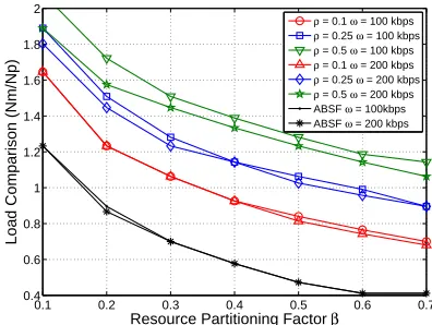
ω. As shown in this figure, the best coverage probability is always achieved when the resource partitioning factor β is approximately0.6. Moreover, the overall rate coverage yields the best performance when using the ABSF. In the ABSF case, the cell range expansion UEs have the best SINR than the others as they suffer no interference from the macro BSs. Thus, a larger expansion area results in more users having better SINR and rate. However, this causes that more UEs are attracted to the pico-cells, as shown in Fig. 10. It illustrates the ratio between the number of macro-cell and pico-cell UEs per-cell when the optimal rate coverage probability is achieved. The ABSF always have more UEs associated with the pico BSs than the LPSF. This means a heavier burden on the back-haul of the pico-cell. However, in practice, the pico-cell may have a limited back-haul while the macro-cell can be assumed unlimited. These optimal biases for a limited back-haul of the pico-cell are not our focus in this work. In the following, we investigate the rate coverage performance with some typical fixed cell range expansion biasesBp.

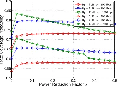
In Fig. 11, we compare the overall rate coverage with a variety of resource partitioning factor β, in terms of some typical range expansion biases Bp (3 dB, 7 dB and 12 dB).

0.1 0.2 0.3 0.4 0.5 0.6 0.7 0.45

0.5 0.55 0.6 0.65 0.7 0.75 0.8 0.85 0.9

Resource Partitioning Factor β

Rate Coverage Probability

ρ = 0.1 Bp = 3 dB ρ = 0.1 Bp = 7 dB ρ = 0.1 Bp = 12 dB ABSF Bp = 3 dB ABSF Bp = 7 dB ABSF Bp = 12 dB

ρ =0.1 Optimised Result ABSF Optimised Result

Fig. 11. Overall rate coverage with varieties ofβin terms of fixedBpwith

ω= 100kbps

0 0.1 0.2 0.3 0.4 0.5 0.5

0.55 0.6 0.65 0.7 0.75 0.8 0.85 0.9

Power Reduction Factor ρ

Rate Coverage Probability

Bp = 3 dB ω = 100 kbps Bp = 7 dB ω = 100 kbps Bp = 12 dB ω = 100 kbps Bp = 3 dB ω = 200 kbps Bp = 7 dB ω = 200 kbps Bp = 12 dB ω = 200 kbps

Fig. 12. Overall rate coverage with varieties ofρ

expansion bias is static, in particular when it is small, the LPSF with a relative low power have limited effects on the rate performance of the cell range expansion users. On the other hand, the rate of the edge macro-cell users increases by sharing more spectrum resources.

In Fig. 12, the rate performance is analysed with a variety of power reduction factor ρ, with the typical values of range expansion bias Bp and rate threshold ω. On one hand, the

result shows that a sharp increase occurs when the ρ varies from 0. Intuitively, compared with the ABSF, the LPSF provide better rate coverage for the macro-cell edge users by sharing more spectrum, but worse rate coverage for the cell range expansion users. In our case, the transmitting power of the LPSF is low, thus the rate coverage gain in the macro-cells exceeds the loss in the pico-macro-cells, which results in the sharp increase of the overall rate coverage performance. On the other hand, interestingly the performance remains almost constant with various ρ (ρ 6= 0) values when the range expansion bias Bp is relatively low. In such a low Bp case,

the number of the CRE UEs is small, and by allocating some more resources to these UEs, the rate coverage loss due to their degraded SINR is made up. In other words, by adjusting the resource partitioning factorβ, the coverage performance is not affected by power reductionρwhen the range expansion bias

is low (under7dB in our simulation). However, a larger range expansion bias results in more UEs to camp to the pico-cell in its expansion region, which will be significantly interfered when the transmitting power of the LPSF is large. Therefore, the coverage performance declines with the increase of the power reduction factor ρ when the range expansion bias is large.

V. CONCLUSION

In this paper we have obtained the analytical results to calculate the overall SINR and rate coverage performance employing the LPSF in the FeICIC. Following the results, the overall rate coverage performance is analysed with the biases, the power reduction factor and the resource partitioning factor. We conclude that with the optimal center and cell range expansion biases, the ABSF outperform the LPSF in terms of both SINR and rate coverage. As the ABSF scheme has a larger optimal CRE bias, more UEs will be attracted to the CRE regions. This will result in a heavier back-haul burden on the pico-cells, which in practice may have limited back-haul capability. The impact of limited back-back-haul on HetNet performance will be studied in our future work. Moreover, if the range expansion bias is static and not optimal, the LPSF in turn outperform the ABSF in terms of rate coverage performance, by sharing more spectrum resource in the macro-cell edge region. Furthermore, when the macro-cell range expansion bias is relatively low (under7dB), the power reduction factor has negligible effect on the rate coverage when the resource partition factor is adjusted.

ACKNOWLEDGEMENT

This paper acknowledges the support of the MOST of China for the ”Small Cell and Heterogeneous Network Planning and Deployment” project (No. 2015DFE12820), the WiNDOW research project supported by the European Commission un-der its 7th Framework Program (No. 318992), the National Natural Science Foundation of China (No. 61571073), the Na-tional High Technology Research and Development Program of China (No. 2014AA01A701), and the China Scholarship Council(CSC). Also, we would like to thank the anonymous reviewers whose constructive and detailed comments helped us a lot to improve the quality of this paper.

APPENDIXA PROOF OFLEMMA1

Firstly, the PDF of two-point distance frj(r) in PPP is

2πλjrexp(−πλjr2) [5]. Prob(ri > krj) could be

compre-hended as the probability, for an arbitrary point in Θi, of no

point is closer thankrj. Then the expression is given as

Prob(ri> krj)

=Prob{no point closer thankrj|rj}

=

Z ∞

0

exp(−λiπk2r2)frj(r)dr

= 2πλj

Z ∞

0

exp(−πr2(λik2+λj))rdr

= λj

λj+k2λi

.

APPENDIXB PROOF OFLEMMA3

The Laplace transformLIi(s)of the aggregate interference

Ii with distance larger thankr is given as:

LIi(s) =E(exp(−sIi))

=E



 Y

i|ri>kr

exp(−sPihr−i αi)





(a) = exp

−2πλi

Z ∞

kr

(1−Ehexp(−sPihu−αi))udu

(b) = exp

−2πλi

Z ∞

kr

sPiu−αi

sPiu−αi+µudu)

(c)

= exp −πλi(

sPi

µ )

2

αi

Z ∞

(kr)2₍sPi µ )

−2

αi

1 1 +tαi2

dt

!

= exp

−πλi(

sPi

µ )

2

αi_C((kr)αi₍sPi

µ )

−1 , αi)

,

(35) where step (a) follows from the probability generating func-tional of the PPP and step (b) is derived byh∼exp(µ). Then given t = (µ/sPi)2/αiu2, we get (c). Thus by implying

C(a, b) = R∞

a2/b1/(1 +tb/2)dt, the result is obtained. Next,

in order to numerically evaluate our expression, the approxi-mation ofC(a, b)is investigated in terms ofa. On one hand, for small parameter (a <1), the expression can be given as

C(a, b) =

Z ∞

0

1/(1 +tb/2_)dt−Z

a2/b

0

1/(1 +tb/2_)dt

(a)

= A(b)−t·2F1

1,2 b; 1 +

2 b;−t

b 2

a2/b

0 (b)

≈A(b)−a2/b

1− 2a

b+ 2

,

(36)

where A(b) = R∞

0 (1 +xb/2)−1dx and 2F1(·) is the Gauss

hypergeometric function. Step (a) is calculated by the symbolic integral calculator [17] and step (b) is the first order series expansion of the Gauss hypergeometric function. The smaller the parameter athe closer match to the actual value.

On the other hand, when a is large (a ≥ 1), we can approximate the result as

C(a, b)(=a)t·2F1

1,2 b; 1 +

2 b;−t

b 2 ∞

a2/b

(b)

=B(b)a(2/b−1)2F1(1,1− 2 b; 2−

2 b;a

−1₎

(c)

≈B(b)a(2/b−1)

1−(b−2)a −1

2b−2

,

(37)

where

B(b) =−2Γ(2/b−1)

bΓ(2/b) . (38)

Step (a) is calculated by the symbolic integral calculator [17] and step (b) is achieved by combining (a) in (37) with (9) in [18]. Step (c) follows from the first order series expansion of the Gauss hypergeometric function.

APPENDIXC PROOF OFLEMMA4

From [19], we have the probability mass function of UE number in a macro-cell as

P(N =n) = 3.5

3.5_{Γ(n+ 3.5)(λ}

u/λm)n

Γ(3.5)n!(λu/λm+ 3.5)n+3.5

. (39)

Then using theorem of discrete expectation, the UE number expectation is

E(N) =E(P(N=n))

=

∞

X

n=1

3.53.5_{Γ(n+ 3.5)(λ}

u/λm)n

Γ(3.5)(n−1)!(λu/λm+ 3.5)n+3.5

. (40)

For notation simplicity, use x denotes _λu/λmλu/λm_+3.5, then this original expression can be presented as follows:

E(N) =(1−x)

3.5

Γ(3.5)

∞

X

n=1

Γ(n+ 3.5) (n−1)! x

n

(a)

= (1−x) 3.5

Γ(3.5)

105·π0.5_x 16(1−x)4.5 =λu/λm,

(41)

where step (a) is calculated in Matlab by serial summarize function.

REFERENCES

[1] A. Damnjanovic, J. Montojo, Y. Wei, T. Ji, T. Luo, M. Vajapeyam, T. Yoo, O. Song, and D. Malladi, “A survey on 3GPP heterogeneous networks,”Wireless Communications, IEEE, vol. 18, no. 3, pp. 10–21, June 2011.

[2] D. Lopez-Perez, I. Guvenc, G. de la Roche, M. Kountouris, T. Quek, and J. Zhang, “Enhanced intercell interference coordination challenges in heterogeneous networks,”Wireless Communications, IEEE, vol. 18, no. 3, pp. 22–30, June 2011.

[3] Panasonic, “Performance study on ABS with reduced macro power,” 3GPP TSG-RAN WG1, Tech. Rep., Nov 2011.

[4] B. Soret and K. Pedersen, “Macro transmission power reduction for hetnet co-channel deployments,” inGlobal Communications Conference (GLOBECOM), 2012 IEEE, Dec 2012, pp. 4126–4130.

[5] J. Andrews, F. Baccelli, and R. Ganti, “A tractable approach to coverage and rate in cellular networks,”Communications, IEEE Transactions on, vol. 59, no. 11, pp. 3122–3134, November 2011.

[6] H.-S. Jo, Y. J. Sang, P. Xia, and J. Andrews, “Heterogeneous cellular networks with flexible cell association: A comprehensive downlink SINR analysis,” Wireless Communications, IEEE Transactions on, vol. 11, no. 10, pp. 3484–3495, October 2012.

[7] S. Singh, H. Dhillon, and J. Andrews, “Offloading in heterogeneous networks: Modeling, analysis, and design insights,” Wireless Commu-nications, IEEE Transactions on, vol. 12, no. 5, pp. 2484–2497, May 2013.

[8] S. Singh and J. Andrews, “Joint resource partitioning and offloading in heterogeneous cellular networks,” Wireless Communications, IEEE Transactions on, vol. 13, no. 2, pp. 888–901, February 2014. [9] H. Tang, J. Peng, P. Hong, and K. Xue, “Offloading performance of

range expansion in picocell networks: A stochastic geometry analysis,” Wireless Communications Letters, IEEE, vol. 2, no. 5, pp. 511–514, 2013.

[10] Q. Ye, B. Rong, Y. Chen, M. Al-Shalash, C. Caramanis, and J. G. Andrews, “User association for load balancing in heterogeneous cellular networks,” Wireless Communications, IEEE Transactions on, vol. 12, no. 6, pp. 2706–2716, 2013.

[11] B. Soret, H. Wang, K. Pedersen, and C. Rosa, “Multicell cooperation for LTE-Advanced heterogeneous network scenarios,”Wireless Commu-nications, IEEE, vol. 20, no. 1, pp. 27–34, February 2013.

[13] T. Novlan, R. Ganti, A. Ghosh, and J. Andrews, “Analytical evaluation of fractional frequency reuse for heterogeneous cellular networks,” Communications, IEEE Transactions on, vol. 60, no. 7, pp. 2029–2039, July 2012.

[14] M. Cierny, H. Wang, R. Wichman, Z. Ding, and C. Wijting, “On number of almost blank subframes in heterogeneous cellular networks,”Wireless Communications, IEEE Transactions on, vol. 12, no. 10, pp. 5061–5073, October 2013.

[15] F. Baccelli and B. Blaszczyszyn, Stochastic Geometry and Wireless Networks, Volume I -Theory. Hanover, MA, USA: NOW Publisher, 2009.

[16] H. S. Dhillon, R. K. Ganti, F. Baccelli, and J. G. Andrews, “Modeling and analysis of K-tier downlink heterogeneous cellular networks,” Se-lected Areas in Communications, IEEE Journal on, vol. 30, no. 3, pp. 550–560, 2012.

[17] W. M. 9. Symbolic integral computation. [Online]. Available: http://www.wolfram.com/mathematica

[18] N. M. Temme, “Large parameter cases of the Gauss hypergeometric function,” Journal of Computational and Applied Mathematics, vol. 153, no. 12, pp. 441 – 462, 2003, proceedings of the 6th International Symposium on Orthogonal Poly nomials, Special Functions and their Applications, Rome, Italy, 18-22 June 2001.