White Rose Research Online URL for this paper:
http://eprints.whiterose.ac.uk/117778/
Version: Accepted Version
Article:
Fu, W and Nijhoff, FW (2017) Direct linearizing transform for three-dimensional discrete
integrable systems: the lattice AKP, BKP and CKP equations. Proceedings of the Royal
Society A: Mathematical, Physical and Engineering Sciences, 473 (2203). 20160915. ISSN
1364-5021
https://doi.org/10.1098/rspa.2016.0915
© 2017 The Author(s). Published by the Royal Society. This is an author produced version
of a paper published in Proceedings of the Royal Society A: Mathematical, Physical and
Engineering Sciences. Uploaded in accordance with the publisher's self-archiving policy.
[email protected] https://eprints.whiterose.ac.uk/
Reuse
Items deposited in White Rose Research Online are protected by copyright, with all rights reserved unless indicated otherwise. They may be downloaded and/or printed for private study, or other acts as permitted by national copyright laws. The publisher or other rights holders may allow further reproduction and re-use of the full text version. This is indicated by the licence information on the White Rose Research Online record for the item.
Takedown
If you consider content in White Rose Research Online to be in breach of UK law, please notify us by
systems: The lattice AKP, BKP and CKP equations
Wei FU and Frank W NIJHOFF
School of Mathematics, University of Leeds, Leeds LS2 9JT, UK
Abstract
A unified framework is presented for the solution structure of 3D discrete integrable systems, including the lattice AKP, BKP and CKP equations. This is done through the so-called direct linearising transform which establishes a general class of integral transforms between solutions. As a particular application, novel soliton-type solutions for the lattice CKP equation are obtained.
Keywords: direct linearising transform, discrete integrable system, discrete AKP equation, discrete BKP equa-tion, discrete CKP equaequa-tion, soliton
1
Introduction
Discrete integrable systems have played an increasingly prominent role in both mathematics and physics during the past decades, cf. e.g. [15]. The theory of discrete integrable systems has made important contributions to other areas of classical and modern mathematics, such as algebraic geometry, discrete geometry, Lie algebras, cluster algebras, orthogonal polynomials, quantum theory, special functions, and random matrix theory.
Discrete equations in a sense play the role of master equations in integrable systems theory. They encode entire hierarchies of corresponding continuous equations and can be understood as the Bianchi permutability property and B¨acklund transforms of both continuous and discrete equations. Furthermore, they have quite significance in their own right, in view of the rich algebraic structure behind them.
A key feature of the integrability of discrete systems is the phenomenon ofmulti-dimensional consis-tency (MDC) – the property that a lattice equation can be consistently extended to a family of equations by introducing an arbitrary number of discrete independent variables with their corresponding lattice pa-rameters, cf. [10, 31]. The MDC property was later employed to classify scalar affine-linear quadrilateral equations [1] and octahedral equations [2] by Adler, Bobenko and Suris.
At the current stage, 3D lattice integrable equations are often considered as the most general models in discrete integrable systems theory – 2D and 1D discrete integrable systems can normally be obtained from dimensional reductions of 3D equations. In fact, the algebraic/solution structures behind 3D lattice equations are much richer and sometimes they provide us with insights into the study of discrete integrable systems, while on the 2D/1D level a lot of key information collapses and the integrability sometimes cannot be easily figured out. Under the assumption of the MDC, there are three important scalar models of Kadomtsev–Petviashvili-type (KP) in the 3D theory, namely, the lattice AKP, BKP and CKP equations, which are the discretisations of the famous continuous (potential) AKP, BKP and CKP equations
4uxt−3uyy−(uxxx+ 6u2x)x= 0, (AKP)
9uxt−5uyy+ (−5uxxy−15uxuy+uxxxxx+ 15uxuxxx+ 15u3x)x= 0, (BKP)
9uxt−5uyy+ (−5uxxy−15uxuy+uxxxxx+ 15uxuxxx+ 15u3x+454u 2
xx)x= 0. (CKP)
Here the letters ‘A’, ‘B’ and ‘C’ refer to the different types of infinite-dimensional Lie algebras which are associated with their respective hierarchies following the work of the Kyoto school, cf. a review paper [17] and references therein for their original research papers. The lattice AKP equation was first given by Hirota [16] in the discrete bilinear form and therefore it is also known as the Hirota equation (also referred to as the Hirota–Miwa equation due to Miwa’s reparametrisation [24] for its soliton solution). The lattice AKP equation is related to other nonlinear forms which can be referred to as the lattice KP equation [28, 29], the lattice modified KP (mKP) equation [6, 28] as well as the lattice Schwarzian KP (SKP) equation – a lattice equation in the form of a multi-ratio (see [11]). The lattice BKP equation was derived by Miwa [24] (therefore also referred to as the Miwa equation) as a four-term bilinear equation and its nonlinear form in terms of multi-ratios was later given by Nimmo and Schief [33] (see also [34]). The lattice CKP equation was obtained from the star-triangle transform in the Ising model by Kashaev [20] based on the idea of nonlocal Yang–Baxter maps [23]. It was named CKP by Schief [35] who revealed that Kashaev’s lattice model is the superposition property of the continuous CKP equation.
We note that the MDC property of the Hirota–Miwa equation and the Miwa equation, i.e. the lattice AKP and BKP equations, can be proven by direct computation, however, the MDC property of the lattice CKP equation (as an equation in multi-quadratic form) is highly nontrivial and it was confirmed in [36]. Alternatively, Atkinson established the MDC property of the lattice CKP equation by using discriminant factorisation [3]. The reductions of the lattice KP-type equations give rise to a large number of lower-dimensional integrable models (cf. e.g. [15] and references therein). In particular, the ultradiscretisations of the reduced 2D lattice integrable models as well as Yang–Baxter maps can be obtained from them [18, 19].
The lattice AKP, BKP and CKP equations have been considered from the perspective of the underlying geometry in several papers, cf. Konopelchenko and Schief [21, 22, 35], Doliwa [7–9] and also Bobenko and Schief [4, 5]. In the present paper, we propose a unified framework for the solution structure of these equations. The latter will comprise the structure of soliton-type solutions and those related to nonlocal Riemann–Hilbert problems. As a particular by-product, we obtain novel soliton solutions to the lattice CKP equation. The approach we adopt is thedirect linearisation (DL) method, which was proven very effective in establishing solution structures of many integrable equations and their interrelations, cf. e.g. [12, 13, 28–30].
The starting point in the DL is a linear integral equation. In the 3D case, we need a singular nonlocal integral equation which reads
uk+
ZZ
D
dζ(l, l′
)ρkΩk,l′σ
l′u
l=ρkck, (1.1)
where dζ(l, l′) is a certain measure for the double integral on an integration domain D in the space of
the spectral variablesl andl′, and the wave functionu
k is an infinite vector with its entries as functions
of discrete dynamical variables as well as the spectral variablekandck is also an infinite vector with its
ith-componentki. Ω
k,l′ is called the Cauchy kernel whileρ
k andσl′ are the plane wave factors. The key
point in this approach is that the measure dζ(l, l′) depends onlandl′and therefore a double integral must
be involved. Once the measure collapses the integral equation turns out to be a local Riemann–Hilbert problem and 2D lattice integrable equations arise.
A more general form of the DL is the direct linearising transform (DLT), cf. [25, 27], which plays the role of a dressing operation in the framework. Concretely, the DLT is a linear transform that maps a solution of the linear problem to another and simultaneously its nonlinear counterpart also brings a solution of the nonlinear equation to a new solution, i.e. one can start from a seed and then generate more and more complicated solutions by iteration. Particularly, when the free wave is chosen to be the seed of the linear problem, the problem turns out to be the integral equation (1.1) which brings us the nonlinear equation together with its solutions.
tantamount to the integrability of the scheme. The crucial aspect of the path-independence of the kernel is equivalent to a closure relation in our infinite matrix structure; it is this closure relation that forms the key condition on the construction of various 3D discrete integrable systems. As the three prominent scalar 3D lattice integrable equations, the lattice AKP, BKP and CKP equations emerge from the scheme together with their associated linear problems. Soliton solutions are obtained by specifying appropriate integration measures and domains.
The paper is organised as follows: In Section 2 we establish the DLT for general 3D discrete integrable systems and its relation to the DL. Sections 3, 4 and 5 are contributed to the lattice AKP, BKP and CKP equations which are corresponding to the three particular cases under the general framework of the DLT. In Section 6, soliton solutions to the lattice AKP, BKP and CKP equations are given from the scheme.
2
A general framework: Direct linearising transform
2.1
Infinite matrices and vectors
Infinite matrices and vectors are the key ingredients in the framework. A matrix/vector is normally understood as an array of numbers, symbols, etc. In fact, such a visualisation is not necessary for describing the essential structure of matrices and vectors, we here present an alternative presentation which is more suitable for the purpose of this paper. This involves the use of infinite “centred” matrices which are built by means of objects (generators) Λ, tΛ and O in an associative algebra (with unit)A
over a fieldF, obeying the relation
O·tΛi·Λj·O=δ−i,−jO, i, j∈Z, (2.1)
where the powers tΛi and Λj are theith andjth compositions oftΛand Λrespectively, and δ
·,· is the
usual Kronecker symbol. In general,Λ,tΛandOdo not commute, but from (2.1) it can be seen thatΛ
andtΛact as each other’s transpose, whileO is a projector satisfyingO2 =O. An, in general, infinite
matrixUis defined as
U= X
i,j∈Z
Ui,jΛ−i·O·tΛ−j, (2.2)
where the coefficients Ui,j take values in the field F. TheUi,j can be understood as the (i, j)-entry in
the infinite matrix and{Λ−i·O·tΛ−j|i, j∈Z}forms a basis. In particular,Oitself can be visualised as
an infinite matrix having the (0,0)-entry 1 and all the other entries zero. Following from (2.1), we can show that operations of these infinite matrices such as addition, multiplication of two infinite matrices as well as scalar multiplication of an infinite matrix byp∈ F obey the following rule:
U+V= X
i,j∈Z
(Ui,j+Vi,j)Λ−i·O·tΛ−j, pU=
X
i,j∈Z
(pUi,j)Λ−i·O·tΛ−j,
U·V= X
i,j∈Z
X
i′∈
Z
Ui,i′V
i′
,j
Λ−i·O·tΛ−j.
In addition, the transpose of U is defined astU =P
i,j∈ZUi,jΛ
−j·O·tΛ−i. The action (·)
0,0 on an
arbitrary infinite matrix defines the centre of the matrixU by taking the coefficient ofΛ0·O·tΛ0, i.e.
(Λi·U·tΛj)
0,0=Ui,j. In particular, we have the following formula:
(Λi1
·U·tΛj1
·O·Λi2
·U·tΛj2
)0,0=Ui1,j1Ui2,j2.
In fact, from the definition (2.2), one can also observe that Λ and tΛ play the role as index-raising
operators from the left and from the right respectively, as we have
Λi′·U·tΛj′
= X
i,j∈Z
Ui+i′
,j+j′Λ
We note that the definition (2.2) also covers finite matrices by restricting the number of non-zero coeffi-cients to a finite number, i.e. Ui,j = 0 for i6= 1,2,· · · , N or j 6= 1,2,· · · , N′ for some givenN andN′,
resulting in anN×N′ finite matrix given byU=PN,N
′
i=1,j=1Ui,jΛ−i·O·tΛ−j.
Following from the same idea, we also introduce infinite vectors as follows. Supposeoandtoare two
objects obeying the relations
to·tΛi·Λj·o=δ
−i,−j, o·to=O, (2.3)
wherei, j∈Zand objectso,to,ΛandtΛdo not commute with each other in general. An infinite vector
uand its transposetuare defined as
u=X
i∈Z
uiΛ−i·o, tu=
X
i∈Z
uito·tΛ−i, (2.4)
where ui are elements in the same field F, which implies o and to are a particular infinite “centred”
vector and its transpose that have the 0th-component (i.e. the centre) 1 and all the other components zero. The sets{Λ−i·o|i∈Z}and{to·tΛ−i|i∈Z}form the respective bases for infinite vectors and their
transpose. For two arbitrary infinite vectors u=Pi∈ZuiΛ
−i·o andv =P j∈ZvjΛ
−j·o where u i, vj
are elements from the field F and for arbitrary p also fromF, we have the basic operations for infinite vectors as follows:
u+v=X
i∈Z
(ui+vi)Λ−i·o, pu=
X
i∈Z
(pui)Λ−i·o,
utv= X
i,j∈Z
uivjΛ−i·O·tΛ−j, tv u=
X
i∈Z
uivi,
as they can be derived immediately by considering the rules in (2.3). The operations obey the same rules (excepti, j are now chosen fromZ) as those for finite vectors. In fact, the case ofN-component (column and row) vectors is obtained by the restrictionui= 0 fori6= 1,2,· · · , N, leading tou=PNi=1uiΛ−i·o
andtu=PN
i uito·tΛ−i. For infinite vectors, we define the action (·)0by taking the coefficient ofΛ0·o
and ofto·tΛ0foruandturespectively, namely (Λi·u)
0=ui and (tu·tΛj)0=uj. The action ofΛand tΛas index-raising operators can be most clearly seen by introducing monomial eigenvectorsc
k andtck′
defined by
Λ·ck =kck, tck′·tΛ=k′tc
k′ and (c
k)0= 1, (tck′)0= 1, (2.5)
from which it implies that the ith-components for the eigenvectors are ki and k′i, respectively. The
monomial basis allows us to encodek- andk′-dependent objects that occur in the integral equation (1.1)
in terms of infinite matrices and vectors and work with them conveniently in a formal manner.
Following the rules (2.1) and (2.3), the multiplication of an infinite matrix and an infinite vector is also well-defined and it obeys exactly the same rule as that in the theory of finite matrices and vectors. Some examples involving both infinite matrices and vectors are given below:
(Λi1
·U·tΛj1
·O·Λi2
·u)0,0=Ui1,j1ui2,
tc
k′·tΛj·O·Λi·c
k =kik′j.
In the approach we also need the notion of trace and determinant of an infinite matrix, but only in the case when they involve the projectorO. Thus we have for the trace Tr(U·O) = Tr(O·U) = (U)0,0and
for the determinant
det(1 +U·O·V) = det(1 +U·o·to·V) = 1 +to·V·U·o= 1 + (V·U)
0,0, (2.6)
where we treatU·oandto·Vas an infinite column vector and an infinite row vector respectively and
2.2
Direct linearising transform for 3D lattice equations
We consider an infinite-dimensional regular lattice spanned by discrete coordinates (called the lattice variables) n1, n2, n3,· · · (for the sake of this paper, taking integer values), each of which is associated
with a corresponding lattice parameterpγtaking values in the reals or the complex numbers (we can think
of pγ representing a grid width parameter in the nγ-direction of the lattice). A discrete shift operator
is defined as follow. Suppose f =f(n1, n2, n3,· · ·) is a function of the discrete independent variables
{n1, n2, n3,· · · }, the discrete forward shift operator Tpγ and the discrete backward shift operator T−pγ1
are respectively defined by
Tpγf =. f(n1, n2,· · · , nγ+ 1,· · ·), T
−1
pγf
.
=f(n1, n2,· · ·, nγ−1,· · ·).
For a 3D discrete integrable system, we only need three discrete independent variables. Thus we can choose an arbitrary triplet (nα, nβ, nγ) from{n1, n2, n3,· · · }as the discrete variables and (pα, pβ, pγ) is
the corresponding triplet for the associated lattice parameters. We consider a family of linear equations taking the form of
Tpuk = (Lp−TpU·Op)·uk, tuk′ = Tptu
k′·(tL
p+Op·U), p∈ {pγ|γ∈Z+}, (2.7)
where the wave functions uk and tuk′ are an infinite column vector and an infinite row vector
respec-tively composed of corresponding entriesu(ki)andu(kj′) as functions of the discrete independent variables
{n1, n2, n3,· · · } and of certain spectral parametersk and k′ which take values in the complex numbers
(we prefer to denote the dependence onkandk′ inu
k,tuk′ by suffices in order to make it more visible).
The potentialUis an infinite matrix with entriesUi,jas certain functions of only the discrete independent
variables{n1, n2, n3,· · · }. The operatorsLpandtLp are expressions ofΛandpandtΛandprespectively andOp is an expression of the operatorsΛ,tΛandOassociated with the lattice parameter p. We note that while theLp commute among themselves for arbitraryp, and so do thetLp, they do not commute with theOp. This follows from the commutativity and noncommutativity ofΛ,tΛandO.
It is not obvious that (2.7) constitutes a compatible system of linear equations, i.e. they can be imposed simultaneously on one and the same function uk or tuk′ respectively. The compatibility of
the system depends sensitively on the choice of Lp, tL
p and Op. The aim is to find choices of these operators for which the compatibility holds and the framework that we set up in this subsection gives necessary conditions for selecting such operators. Furthermore, the requirement of compatibility also imposes conditions on the coefficient matrix U, namely for each triplet (pα, pβ, pγ), the compatibility
conditions TpαTpβuk = TpβTpαuk and TpβTpγuk = TpγTpβuk leads to a formal 3D lattice system for
the infinite matrixUwith entries as functions of the triplet (nα, nβ, nγ) chosen from the{n1, n2, n3,· · · }:
(Lpα−TpβTpαU·Opα)·(Lpβ−TpβU·Opβ) = (Lpβ−TpαTpβU·Opβ)·(Lpα−TpαU·Opα), (2.8a)
(Lpβ−TpγTpβU·Opβ)·(Lpγ−TpγU·Opγ) = (Lpγ−TpβTpγU·Opγ)·(Lpβ−TpβU·Opβ). (2.8b)
At this juncture we need to point out that (2.8) can only be considered as a closed-form lattice equation in the sense of the infinite matrixU, but it is not closed-form for individual entries in the matrix, since the operatorsLp,tL
p andOp in general contain the index-raising operatorsΛandtΛ. Thus, in order to obtain closed-form 3D lattice equations for the entries of Uthe latter operators must be eliminated. In Sections 3, 4 and 5, we specify the operators Lp,tL
p and Op and derive the corresponding closed-form lattice equations. What we do here is to set up the solution structure behind these equations which will make transparent the integrability in the sense of the MDC property.
Let us explain what we mean by the MDC property in this context. Consider an, in principle infinite, family of equations arising from (2.8), each involving a triplet (pα, pβ, pγ) as lattice parameters and
an associated triplet (nα, nβ, nγ) as lattice variables arbitrarily chosen from the infinite sets of lattice
parameters and variables{pγ|γ∈Z+}and{nγ|γ∈Z+}, the MDC is the property that this family admits
parameters). In the following, we show that the MDC property is only guaranteed whenLp,tL
p andOp satisfy certain conditions which are governed by the DLT.
We introduce the DLT, namely, a linear transform from the given wave functionsu0k,tu0
k′ to new wave
functionsuk,tuk′ in the form of
uk=u0k−
ZZ
D
dζ(l, l′
)G0k,l′ul, tuk′ =tu0
k′ −
ZZ
D
dζ(l, l′
)Gl,k′tu0
l′, (2.9)
in whichDis a suitable integration domain and dζ(l, l′) is the measure. G0
k,l′ andGl,k′ are the kernel of
the DLT that must obey a certain condition which will be given later. The idea of the DLT is that the transform must preserve the structure of the linear equations in (2.7), i.e. if we start from an old solution
u0k,tu0
k′ to (2.7) together withU0, the newuk and tuk′ that follow from the linearising transform (2.9)
must satisfy the same linear problem associated with a newU. Such a requirement leads that the kernel
Gmust obey
(Tp−1)G0k,l′ = (Tptu0
l′)·Op·u0
k, (Tp−1)Gl,k′ = (Tptu
k′)·O
p·ul (2.10)
for anyp∈ {pγ|γ∈Z+}, which implies that it is defined as
G0k,l′ =
X
ΓP→X
(Tptu0l′)·O
p·u
0
k, Gl,k′ =
X
ΓP→X
(Tptuk′)·O
p·ul, (2.11)
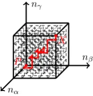
where Γ is an arbitrary path from the initial point P to the ending pointX in the lattice and the path must follow the lattice directions (cf. Figure 1 as a particular case when the path is sitting in a 3D lattice spanned by the coordinatesnα,nβ andnγ). Simultaneously there is also a nonlinear counterpart of the
DLT (2.9) that must hold, namely, a transform between the oldU0 and the newU, which is given by
U−U0=
ZZ
D
dζ(l, l′
)ultu0l′. (2.12)
The transform (2.12) together with the equations in (2.7) also implies thatU must obey
(TpU−TpU0)·(tLp+Op·U
0) =L
p·(U−U
0)−(TpU)·O
p·(U−U
0). (2.13)
The relation (2.13) is a nonlinearised version of (2.7) and it describes how the nonlinear quantities U
and U0 evolve along the lattice directions. And it can also bring us closed-form 3D lattice systems by selecting a certain entry (for scalar 3D lattice equations) or several certain entries (for coupled 3D lattice systems) of the infinite matrixUonce the initial conditionU0 is given – the simplest choice isU0=0
as we can easily observe that from (2.8).
nα
nβ
nγ
P
[image:7.595.239.332.583.679.2]X
Fig. 1: An arbitrary path Γ in the 3D lattice space
The equations in (2.9) together with (2.12) constitute a dressing method for solving the 3D lattice nonlinear equation (2.8): We can start from a seed of the nonlinear equation, say U0, then (2.7) can be solved and we obtain its seed solution u0k and tu0
k′. Next the kernel G0
(2.11). Then the linearising transform (2.9) gives us the new solution uk to the linear problem and consequently the new solution U to the nonlinear equation can be worked out from (2.12). We can repeat the procedure from the obtained new solution and create more and more complicated solutions by iteration. The iteration can be illustrated in the diagram as follow:
U0 U1 U2
↓ ↑ ↑
u0k,tu0
k′ −→ u1
k −→ u2k −→ · · ·
(2.14)
The DLT procedure including (2.9) and (2.12) provides a way of generating solutions to (2.8), starting from an initial solution. In order to find nontrivial solutions admitting infinitely many degrees of freedom which can solve all the discrete equations for U in the family (i.e. the MDC property), we must have that the kernelGin the DLT given by (2.11) is path-independent, namely a closure relation at each stage in the dressing:
(Tq−1)(Tp−1)Gk,l′ = (Tp−1)(Tq−1)G
k,l′, ∀p,q∈ {p
γ|γ∈Z+}.
Following from (2.10) and making use of (2.7), one can from the above relation derive a closure relation forL·, tL· andO·by eliminating Tpuk and Tquk (but reserve TpTquk and uk). The statement can be
made as follow:
Proposition 2.1. A 3D lattice equation from (2.8)possesses the MDC property if the operators L·,tL·
andO· obey the closure relation
OpLq−tLqOp=OqLp−tLpOq, ∀p,q∈ {pγ|γ∈Z+}. (2.15)
The statement holds because the closure relation (2.15) is equivalent to the path-independence of the kernel G, namely the DLT preserves the structure of the family of the linear equations (2.7) as well as the family of the nonlinear equations (2.8). In other words, a general solution solving the hierarchy of the discrete equations inUcan be obtained from the DLT if we start from a common seed solution, i.e. the zero solutionU0=0, where an arbitrary number of degrees of freedom can be introduced (from the measure) during the DLT iteration (2.12), cf. Section 6 for soliton solutions.
Another comment is that Equation (2.15) needs to be understood as an equation for the triplet (L·,tL·,O·). Since it is not fully determined, it might be difficult to find its general solution. Nevertheless,
one needs to keep the commutativity and noncommutativity properties of the operators in mind and some particular solutions can be expected from the closure relation. In fact, any solution of the closure relation (2.15) can result in a 3D lattice integrable equation and we shall see in the following sections that even some simple solutions can generate highly nontrivial 3D discrete integrable systems.
We can see from the dressing procedure that the kernel G of the DLT is the key quantity in the approach. In fact, it possesses a very important property, namely, the kernel itself obeys a closed relation. We propose the statement in the following lemma:
Lemma 2.1. The kernelGof the DLT obeys itself an integral equation
Gk,k′ =G0
k,k′−
ZZ
D
dζ(l, l′
)Gl,k′G0
k,l′. (2.16)
Proof. We can expand Gk,k′ following the definition (2.11) and replace u
k and tuk′ by u0
k and tu0k′
respectively according to the DLT (2.9). Thus one obtains
Gk,k′(X) =G0
k,k′(X)−
ZZ
D
dζ(l, l′
) X
ΓP→X
X
ΓP→X′
Tqtu k′(X
′′
)·Oq·ul(X′′)
Tptu0
l′(X
′
)·Op·u0k(X
′
)
−
ZZ
D
dζ(l, l′
) X
ΓP→X
X
ΓP→X′
Tqtu0l′(X
′′
)·Oq·u
0
k(X
′
)Tptuk′(X′)·O
where X denotes the argument {n1, n2, n3,· · · },X′, X′′ denote summed over positions along the paths
ΓP→X and ΓP→X′ respectively, and T·is the elementary discrete shift associated with the lattice
param-eterspandq governed by the paths. The identity that one needs for the proof is
X
ΓP→X
X
ΓP→X′
A(X′′
+ep′′, X
′′
)B(X′
+ep′, X
′
) + X
ΓP→X
A(X′
+ep′, X
′
) X
ΓP→X′
B(X′′
+ep′, X
′′
)
= X
ΓP→X
A(X′
+ep′, X′)
X
ΓP→X
B(X′′
+ep′′, X′′)
, (2.17)
whereep′ ande
p′′are elementary discrete shifts andA,Bare functions defined on the infinite-dimensional
lattice. We note that the identity is nothing but a discrete version of integration by part. Now the double summation in the above equation ofGcan be reformulated as a product of two summations and the right hand side of the equation turns out to be
G0k,k′(X)−
ZZ
D
dζ(l, l′
) X
ΓP→X
Tqtu0
l′(X
′′
)·Oq·u
0
k(X
′′
) X
ΓP→X
Tptu
k′(X′)·O
p·ul(X′)
,
which implies the integral equation ofGholds if one follows the definition (2.11).
With the help of (2.16), one can actually establish a group-like property for the general DLT. We propose it in the following theorem:
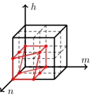
Theorem 2.1. The DLT for a 3D lattice equation, i.e. (2.9) and (2.12), satisfies a group-like property (see Figure 2) in the sense that for two arbitrary DLTs
(U0,u0k,tu0k′)−→(U
1,u1
k,tu1k′) and (U
1,u1
k,tu1k′)−→(U
2,u2
k,tu2k′)
with respect to the domains and the measures(D10,dζ10(l, l′))and(D21,dζ21(l, l′))respectively, the
trans-form between (U0,u0k,tu0
k′)and(U2,u2
k,tu2k′)follows
u2k =u0k−
ZZ
D20
dζ20(l, l′)G0k,l′u
2
l, tu2k′ =
tu0
k′−
ZZ
D20
dζ20(l, l′)G2l,k′
tu0
l′,
U2−U0=
ZZ
D20
dζ20(l, l′)u2ltu
0
l′, where
ZZ
D20
·dζ20(l, l′)=. ZZ
D21
·dζ21(l, l′) + ZZ
D10
·dζ10(l, l′).
Proof. One just needs to eliminateu1k andtu1
k′ in the dressings “0→1” and “1→2” and simultaneously
replacesG1 byG0(orG2), using (2.9) as well as the integral equation (2.16).
D10,dζ10(l, l
′
) D21,dζ21(l, l
′
) (u0
k,u
0
k′,U
0
) (u1
k,tu
1
k′,U
1
) (u2
k,tu
2
k′,U
2 )
D20,dζ20(l, l
′
[image:9.595.76.510.172.230.2])
Fig. 2: Group-like property of the DLT
Theorem 2.1 brings to light the underlying integrability of the structure. In fact, it implies that solutions from successive applications of the DLT are compatible.
2.3
Infinite matrix structure of the direct linearisation
To recover the DL from the DLT, the wave functions must be chosen to be the free waves. In fact, we need a seed solution to the nonlinear equation, i.e. the zero solutionU0=0. Then the free wave solution
u0k, tu0
k′ can be solved from the original linear problem (2.7) and they take the form ofu0
k =ρkck and tu0
k′ = tck′σ
k′ respectively, where c
k and tck′ are the monomial eigenvectors defined in (2.5), and the
plane wave factorsρk andσk′, as functions dependent on the lattice variables and parametersn
γ andpγ,
and also the spectral parametersk andk′
respectively, are defined by
(Tpρk)ck =ρkLp·ck, tck′σ
k′ =tc
k′·tLp(Tpσ
k′), p∈ {p
γ|γ∈Z+}. (2.18)
Now we define the operatorΩ, an expression ofΛ,tΛandOwhich is independent of the lattice parameter
p, by the following:
Ω·Lp−tLp·Ω=Op, p∈ {pγ|γ∈Z+}. (2.19)
The Cauchy kernel can immediately be recovered from the operatorΩas follow:
Ωk,l′ =tc
l′·Ω·c
k. (2.20)
From the definition of the Cauchy kernel (2.20) it is obvious to see that the operator Ω is the infinite matrix form of the Cauchy kernel. However, we note that the infinite matrix form is much more convenient for us to deal with the computation in practice. With the free waves and the Cauchy kernel, we can now explain the kernelG0
k,l′ of the DLT in this special case. In fact, making use of (2.19) and (2.20) one can
show that
G0
k,l′=
X
ΓP→X
(Tpσl′)tc
l′·O
p·ckρk =
X
ΓP→X
(Tpσl′)tc
l′·(Ω·L
p−tLp·Ω)·ckρk
= X
ΓP→X
((Tpσl′)Ω
k,l′(Tpρ
k)−σl′Ω
k,l′ρ
k) =ρkΩk,l′σ
l′
X
P =ρkΩk,l
′σ
l′, (2.21)
in which the initial point P is set to be −∞(for the sake of soliton-type solutions) in the summation along the path in order to get rid of the constant of summation. This tells us that G0
k,l′ is a quantity
containing both the Cauchy kernel and the plane wave factors. More precisely, the special case brings the DLT (2.9) back to the integral equation (1.1). With the help of the infinite matrix structure, it also makes it possible for us to rewrite the integral equation (1.1) in a more compact form, namely,
uk= (1−U·Ω)·ρkck, (2.22)
whereU=RRDdζ(l, l′)u
ltu0l′ as it follows from (2.12) whenU0= 0. The linear equation (2.22) also leads
to a similar relation for the infinite matrixU:
U= (1−U·Ω)·C, (2.23)
where the infinite matrixC is given by
C=
ZZ
D
dζ(l, l′
)u0ltu0l′ =
ZZ
D
dζ(l, l′
)ρlcltcl′σl′. (2.24)
The quantityC is an analogue of the free wave functions in the infinite matrix structure, which can be understood as a linear version of U. For arbitraryp ∈ {pγ|γ ∈Z+}, the infinite matrix C satisfies the
dynamical relation
(TpC)·tL
Its nonlinear counterpart, i.e. the dynamical relation for the infinite matrixU, can naturally be obtained from the transform ofU(2.12) in the particular case ofU0=0, which now takes the form of
(TpU)·tLp=Lp·U−(TpU)·Op·U, p∈ {pγ|γ∈Z+}. (2.26)
Alternatively, such relations can also be derived from (2.23) together with (2.19) and (2.25).
Equation (2.26) is the fundamental relation for constructing closed-form scalar 3D lattice equations within the DL framework and it is fully characterised by the operators Lp, tL
p as well as Op. The operators are determined by the closure relation (2.15) as we have pointed out in the previous subsection. In the next three sections we consider several particular solutions to the closure relation and show that they surprisingly lead to the well-known lattice AKP, BKP and CKP equations.
3
The lattice AKP equation
As it has been shown that only three discrete independent variables are sufficient to generate a 3D lattice equation from the DLT approach and the obtained lattice equation possesses the MDC property, from now on we fix on the discrete independent variables n=. n1, m=. n2, h =. n3 and the associated lattice
parametersp=. p1, q=. p2, r=. p3without losing generality. Some short-hand notations can be introduced
for simplicity as follows. Suppose f =. fn,m,h =f(n, m, h) is a function defined on the 3D lattice, we
identifye·,b·and ¯·with Tp, Tq and Tr, i.e.
e
f = T. pf =fn+1,m,h, fb= T. qf =fn,m+1,h, f¯= T. rf =fn,m,h+1,
and similarly the undershifts denote the backward shifts, namely,
f
e
.
= T−1
p f =fn−1,m,h, f
b
.
= T−1
q f =fn,m−1,h, f
¯
.
= T−1
r f =fn,m,h−1.
In order to consider a simple nontrivial solution to the closure relation (2.15), we assume that Op is independent of p. The simplest choice is that Op =O. At the same time, we require that Lp and tLp linearly depend on the operatorsΛandtΛrespectively. For nontrivial 3D lattice equations, a simple but
nontrivial choice is
Lp=p+Λ, tLp=p−tΛ, Op=O, p=p, q, r, (3.1) and as a result, the fundamental dynamical relations in (2.26) in this case now turn out to be
e
U·(p−tΛ) = (p+Λ)·U−Ue ·O·U (3.2)
together with the other two relations by the replacements (e·, p) ↔ (b·, q) ↔ (¯·, r). The equation (3.2) together with the analogues associated with the other two lattice directions are the basic relations that describe the evolutions of the infinite matrixU. Closed-from scalar lattice equations in certain entries of
Ucan be obtained from the relations. In order to find these lattice equations, we introduce
u= (U)0,0, v= 1−(U·tΛ−1)0,0, w= 1−(Λ−1·U)0,0, z= (Λ−1·U·tΛ−1)0,0−z0,
wherez0=np+mq +hr. Since Equation (3.2) is a relation for infinite matrices, we can consider [(3.2)]0,0,
[(3.2)·Λ−1]
0,0, [Λ−1·(3.2)]0,0and [Λ−1·(3.2)·tΛ−1]0,0respectively and obtain some dynamical relations
involving the above quantities. By eliminating other redundant variables, the following nonlinear 3D lattice equations, namely the lattice KP, mKP and SKP equations, are derived:
(p−ue)(q−r+ue¯−beu) + (q−ub)(r−p+beu−u¯b) + (r−u¯)(p−q−¯bu−e¯u) = 0, (lattice KP)
pbev
b
v −
e¯v
¯
v
+qv¯b
¯
v −
be
v
e
v
+re¯v
e
v −
¯
b
v
b
v
= 0, (lattice mKP)
p bw
be
w−
¯
w
e¯
w
+qw¯¯
b
w−
e
w
be
w
+r ew
e¯
w−
b
w
¯
b
w
= 0, (lattice mKP)
(zbe−zb)(¯zb−z¯)(e¯z−ze)
We note that the equations inv and ware both the lattice mKP equation and the continuum limit of either gives us the fully continuous mKP equation. If fact, we can transfer one to the other by introducing a simple transform (n, m, h)→(−n,−m,−h). In addition, if we consider s= (Λ−1·U−U·tΛ−1)
0,0,
another scalar closed-form equation can be found and it is given by
p es¯−¯s
(2−e¯s)(2 + ¯s)−
bes−bs
(2−bes)(2 +bs)
!
+q bes−es
(2−bes)(2 +es)− ¯
b
s−s¯ (2−¯bs)(2 + ¯s)
!
+r ¯bs−bs
(2−¯bs)(2 +bs)−
e¯s−es
(2−es¯)(2 +es)
!
= 0. (3.3)
The lattice KP, mKP and SKP equations as well as Equation (3.3) are connected with each other via Miura-type transforms. As a remark, we note that the equations in v, w, z and s can be obtained separately by choosing the sameLp andtLp in (3.1) with slightly differentOp, namely,
Op=tΛ·O, Op=O·Λ, Op=tΛ·O·Λ, Op= 12(O·Λ−tΛ·O), (3.4) respectively. One can even consider more complexOp with the sameLp andtLp and obtain other lattice equations, but they could only exist in multi-component form. In fact, all these lattice equations belong to the lattice AKP class because effectively they can all fit into (3.2) and therefore we can conclude that (3.2) together with its counterparts in the other lattice directions is the fundamental relation to understand the structure hidden behind the lattice AKP equation.
There are some other important forms of the lattice AKP equation. For later convenience we introduce the following new variables:
Va= 1−
U· 1
a+tΛ
0,0, Wa = 1−
1
a+Λ·U
0,0, Sa,b=
1
a+Λ·U·
1
b+tΛ
0,0.
These quantities contain the parametersaandband therefore they are more general and can degenerate to the previous main variables via suitable limits in terms of a and b. One of the most important quantities in the integrable systems theory is theτ-function and it in the lattice AKP case can be defined asτ = det(1 +Ω·C). Here the determinant of the infinite matrix can be worked out according to what we have explained in Section 2. In fact, following from (2.19) and (2.25), we have the dynamical relations forΩandC obeying
Ω·(p+Λ)−(p−tΛ)·Ω=O, (3.5a)
e
C·(p−tΛ) = (p+Λ)·C, (3.5b)
as well as the relations in terms of (b·, q) and (¯·, r). These dynamical relations help us to find the evolutions of theτ-function. Consider the dynamical evolution of theτ-function, one can obtain
e
τ= det[1 +Ω·C+ (p−tΛ)−1·O·C] =τh1 +U· 1
p−tΛ
0,0 i
and a similar relation forτ
e, where (2.6) is used. Therefore we obtain the evolutions of theτ-function as
follows:
e
τ
τ =V−p, τ
e
τ =Wp. (3.6)
where (3.5) is used in the derivation. We note that similar relations also hold for (b·, q) and (¯·, r). Now from (3.2), we can derive the dynamical relations forWa by considering [a+1Λ·(3.2)]0,0, i.e.
p(1−Wfa)−
1
a+Λ·Ue ·
tΛ
as well as the similar relations for (b·, q) and (¯·, r). Such relations give rise to the transform between u
andτ (if we seta=p):
p−q+bu−ue= (p−q)τbeτ
b
τeτ. (3.8)
Similar relations for the other discrete shifts associated with the corresponding lattice parameters can be obtained in the same way. If we eliminateuand replace Wp,Wq andWr by theτ-function, we end up
with the discrete bilinear KP equation
(p−q)beτ¯τ+ (q−r)¯τbeτ+ (r−p)e¯τbτ= 0, (3.9) namely, the Hirota–Miwa equation, cf. [16] (see also [24]). Moreover, (3.2) also gives rise to
1 + (p−a)Sa,b−(p+b)Sea,b=WfaVb, (e·, p)↔(b·, q)↔(¯·, r), (3.10)
if we consider [ 1
a+Λ·(3.2)·
1
b+tΛ]0,0. EliminatingWa andVbin the relation then provides us with a more
general 3D lattice equation which reads
[1 + (p−a)Sba,b−(p+b)Sbea,b][1 + (q−a) ¯Sa,b−(q+b)S¯ba,b][1 + (r−a)Sea,b−(r+b)Se¯a,b]
[1 + (p−a) ¯Sa,b−(p+b)Se¯a,b][1 + (q−a)Sea,b−(q+b)Sbea,b][1 + (r−a)Sba,b−(r+b)S¯ba,b]
= 1. (3.11)
This is an extension of the lattice SKP equation which was given in [29]. The equation can be considered as the most general equation in the AKP class as suitable limits in terms ofaandb of the equation lead to be the lattice KP, mKP and SKP equations as well as the Hirota–Miwa equation (3.9). In fact, the parametersaandbcan be understood as the two extra lattice parameters associated with two auxiliary discrete variables, and bothaandb as well asp, q, rare on the same footing – this is guaranteed by the MDC property. One can therefore find a connection betweenSa,b and theτ-function, which is given by
1−(a+b)Sa,b=
T−1
a T−bτ
τ . (3.12)
Now we consider the linear problem of the lattice AKP equation. The linear equations (2.7) for the lattice AKP equation give us
e
uk= (p+Λ)·uk−Ue ·O·uk, (e·, p)↔(b·, q)↔(¯·, r), (3.13)
which leads to the following equation if we take the centre of (3.13) and setφ= (uk)0:
e
φ−φb= (p−q+bu−eu)φ= (p−q)τbeτ
b
ττeφ, (3.14)
and also the other two similar equations if we interchange (e·, p)↔(b·, q)↔(¯·, r). This is the Lax triplet of the Hirota–Miwa equation. In other words, the compatibility condition of (3.14) gives us (3.9). One comment here is that if we eliminate theτ-function in the Lax triplet, we can obtain a nonlinear form of the lattice AKP equation without the lattice parameters, namely,
be
φ−¯φb
b
φ +
¯b
φ−eφ¯
¯
φ +
e¯
φ−φbe
e
φ = 0, (3.15)
which is nothing but the lattice mKP equation ofvafter a point transform.
In the lattice KP, mKP equations u and v are both potential variables, we would like to note that there also exists a non-potential form of the lattice KP equation. The lattice KP equation can be written in an alternative form which reads
(q−r+ ¯u−ub)e q−r+ ¯u−ub =
(r−p+eu−u¯)b r−p+eu−u¯ =
(p−q+ub−ue)¯
n
[image:14.595.240.332.126.225.2]m h
Fig. 3: The non-potential lattice AKP equation
Due to the above form of the lattice AKP equation, it is very natural for us to introduce the non-potential variables
P =q−r+ ¯u−bu, Q=r−p+eu−u,¯ R=p−q+ub−u,e (3.17) and consequently a coupled system ofP,QandRcan be derived from (3.16), i.e.
e
P P =
b
Q Q =
¯
R
R, P+Q+R= 0, Pe+Qb+ ¯R= 0, (3.18)
where the first equation is Equation (3.16) itself and the other two follow from the definitions ofP,Qand
Rdirectly. The system (3.18) can be treated as the lattice non-potential KP equation and it was proposed by Nimmo in [32]. Now for a scalar form, we first eliminateRand obtain P /Pe =Q/Q,b P¯+ ¯Q=Pe+Qb, and then one can have the expression ofP in terms ofQand consequently the expression ofRin terms ofQ:
P =QQe( ¯Q(Qbe−Qe¯) + ¯
b
Q( ¯Q−Qb))
b
Q(QeQ¯b−Q¯Qbe)
, R=QQ¯(Qe(Qe¯− ¯b
Q) +Qbe(Qb−Q¯))
b
Q(QeQ¯b−Q¯Qbe)
.
Now if we express everything in Q, the system turns out to be a 10-point scalar lattice equation (see Figure 3) in the form of
e
QQeeQbeQ¯beQ¯b−QeeQbeQbe¯QbQ¯b+QeeQbeQbe¯Q¯bQ¯−QeQeeQbeeQ¯bQe¯−QeQeeQbe¯Q¯bQe¯+QbeeQbeQbQ¯bQe¯
+QeeQbeeQbeQ¯Qe¯−QbeeQbe
2
¯
QQe¯−QbeeQbeQ¯bQ¯Qe¯+QbeeQbeQ¯Qe¯2+QeQeeQ¯bQe¯Qee¯−QeeQbeQ¯Qe¯Qee¯= 0. (3.19) It is this quintic equation which we refer to as the non-potential lattice KP equation and this scalar form, to the best of the authors’ knowledge, has not been given elsewhere. The Lax triplet of the equation can be obtained from (3.14) directly if we consider (3.17) and the expressions ofP andRin terms ofQgiven above. We note that a different nonlinear form of the non-potential discrete AKP equation was given in [14] in which the equation is quartic but has 14 terms (compared to our quintic equation having 12 terms).
Before we move onto the lattice BKP and CKP equations, we would like to note that in the AKP class there exist several nonlinear integrable equations which are connected with each other through Miura-type transforms. In fact they are the same equation in different forms because the core part of the scheme, namely, the form of the operatorsLp,tL
wave factors. Therefore in the future we only mean the equation in theτ-function, i.e. the Hirota–Miwa equation (3.9), by the lattice AKP equation. While the other forms of the lattice AKP equation, namely, the equations in u,v, w, Sa,b as well as Equation (3.3) can all be expressed by theτ-function. This is
done by taking suitable limits on the parametersaand bin (3.12). In the next sections, we will mainly be concentrating on theτ-function to understand the structure of the lattice BKP and CKP equations. Furthermore, we also note that the τ-equation does not necessarily need to be bilinear although the terminology was from the bilinear theory.
4
The lattice BKP equation
Now we try to find slightly complex solution to the closure relation (2.15) in order to obtain different classes of 3D lattice integrable equations. As we assumed thatOp =O (the simplest case whenOp is independent of p) and Lp andtLp must linearly depend on Λand tΛ in the lattice AKP class, we now suppose that they depend onΛand tΛfractionally linearly. One of solutions under the assumption can
be
Lp= p+Λ
p−Λ,
tL
p= p−tΛ
p+tΛ, Op =p 1
p+tΛ·(O·Λ−
tΛ·O)· 1
p−Λ, p=p, q, r. (4.1)
In order to understand the 3D lattice equation in this class from the point view of the τ-function, we need the relations forΩandC. According to (2.19) and (2.25), in this case the dynamical evolution for them must obey
Ω·p+Λ
p−Λ− p−tΛ
p+tΛ·Ω=p
1
p+tΛ·(O·Λ−
tΛ·O)· 1
p−Λ, (4.2a)
e
C·p−
tΛ
p+tΛ =
p+Λ
p−Λ·C, (4.2b)
as well as the similar (b·, q)- and (¯·, r)-relations. Equation (4.1) also tells us that the nonlinear evolutions of the infinite matrixUin this class satisfy
e
U· p−
tΛ
p+tΛ =
p+Λ
p−Λ·U−pUe ·
1
p+tΛ·(O·Λ−
tΛ·O)· 1
p−Λ ·U, (4.3)
as well as similar relations for (b·, q) and (¯·, r). These relations can be obtained from (2.26). Now one can try to select certain entries in the matrix U following the idea in the lattice AKP equation and expect to derive some closed-form equations from the framework. However, due toOp now depending on the lattice parametersp, q, r, it is not possible to derive closed-form scalar lattice equations from the relations without any extra conditions and a multi-component form must be involved. In order to get a scalar equation, we impose an extra condition on the relations and it is actually done through imposing a constraint on the measure in the DLT which is given by dζ(l, l′) =−dζ(l′, l). The reason why we impose
the extra condition is that theΩin this case is antisymmetric if one follows (2.19) and (2.20) and we want the measure to match this property. Under this constraint, one can figure out from (2.24) and (2.23) that the infinite matricesCandU satisfy the antisymmetry propertytC=−C,tU=−U. Consequently we
have (Λi·U·tΛi)
0,0 = 0 for arbitrary i∈Z. For simplicity in the future, we here introduce some new
variables as follows:
Va= 1−
U· a
a−tΛ
0,0= 1 +
a
a−Λ·U
0,0=Wa,
Sa,b =
a
a−Λ·U· b b−tΛ
0,0=−Sb,a,
where Va = Wa and Sa,b = −Sb,a due to the antisymmetry property of U. Focusing on these new
[ a
a−Λ·(4.3)· b
b−tΛ]0,0, we derive the following relations as a consequence:
VpVe−p= 1, (4.4a)
1 + 2VpSe−a,−p =
a−p
a+p(Vp−V−a) +VpVe−a (4.4b)
as well as the dynamical relation for the variableSa,b:
b+p
b−pSe−a,−b+ p−a
p+aS−a,−b−
2b
b−pSe−a,−p+
2a p+aSp,−b
+ (1−V−b)Se−a,−p−(1−Ve−a+ 2Se−a,−b)Sp,−b= 0, (4.4c)
together with the dynamical relations along the other two directions, i.e. (b·, q) and (¯·, r). These relations will play the core ingredients for constructing a closed-form lattice equation later. We now introduce the
τ-function and it is defined byτ2= det(1 +Ω·C). Consider the dynamical evolution of theτ-function, we have
e
τ2= det(1 +Ω·Ce) = det1 +Ω·C+p 1
p−tΛ·(O·Λ−
tΛ·O)· 1
p−Λ·C
=τ2det 1 +p(
Λ p−Λ·U·
1
p−tΛ)0,0 −p(p−ΛΛ·U· tΛ
p−tΛ)0,0
p(p−1Λ·U·
1
p−tΛ)0,0 1−p(p−1Λ·U· tΛ
p−tΛ)0,0 !
,
in which we have used the rank 2 Weinstein–Aronszajn formula. The similar relations also hold for (b·, q) and (¯·, r) as well as the undershifts (·
e,−p), (·b,−q) and (·¯,−r). Taking (4.4a) into consideration, without
losing generality, we have the dynamical relations for theτ-function
Vp= e
τ
τ, V−p= τ
e
τ, Vq=
b
τ
τ, V−q= τ
b
τ, Vr=
¯
τ
τ, V−r= τ
¯
τ. (4.5)
Now if we seta=qin (4.4b), theV-variables can be replaced by theτ-function using (4.5), and therefore we can expressS−q,−p byτ in the following formula:
S−q,−p=
1 2
hτ
b−τ τe+qq−+pp
1−τbe
τ
i
. (4.6)
Similar relations in terms of the other lattice parameters and discrete shifts can be obtained in a similar way. Finally, setting a=q and b =r in (4.4c) and replacing everything by the τ-function, we end up with a closed-form 3D lattice equation in theτ-function, which takes the form of
(p−q)(q−r)(r−p)τ¯beτ+ (p+q)(p+r)(q−r)eτ¯bτ
+ (r+p)(r+q)(p−q)¯τbeτ+ (q+r)(q+p)(r−p)bτeτ¯= 0. (4.7) This is the lattice BKP equation which is also known as the Miwa equation [24]. The difference between the Miwa equation and the Hirota–Miwa equation is that the former has an extra term (the fourth term). In fact if one applies some formal limits, the Hirota–Miwa equation can be recovered from the Miwa equation.
Next, we consider the linear problem of the lattice BKP equation. The linear equations (2.7) in the lattice BKP case are given by
e
uk=
p+Λ
p−Λ ·uk−pUe ·
1
p+tΛ·(O·Λ−
tΛ·O)· 1
p−Λ·uk (4.8)
together with its (b·, q) and (¯·, r) counterparts, as Lp, tL
p and Op follow from (4.1). By introducing
φ= (uk)0, ψa = (a−aΛ ·uk)0, we therefore from (4.8) have
e
φ=Ve−p(ψp−φ), ψe−a =
p−a
together with the similar equations associated with (b·, q) and (¯·, r). And now we eliminate ψby setting
a=pand as a result we can derive the Lax triplet of the lattice BKP equation
be
φ−φ=p+q
p−q
bτeτ
τbeτ(φb−φe), (e·, p)↔(b·, q)↔(¯·, r). (4.10)
Similarly, a nonlinear form of the BKP equation can be obtained if we eliminate the τ-function in the Lax triplet and it takes the form of
(¯φb−eφ¯)(φbe−φ) (eφ¯−beφ)(φ−¯φb)
= (φe−φb)( ¯φ− ¯
be
φ) (φb−φ¯)(φ¯be−φe)
, (4.11)
where two cross-ratios are involved in the explicit form.
5
The lattice CKP equation
Under the assumption in Section 4, namely, the operatorsLp,tL
pandOpdepend onΛandtΛfractionally linearly, there is also another solution to the closure relation (2.15):
Lp= p+Λ
p−Λ,
tL
p= p−tΛ
p+tΛ, Op = 2p 1 p+tΛ·O·
1
p−Λ, p=p, q, r. (5.1)
Again, once we have the explicit expressions for the key informationLp,tL
pandOp, the general formula (2.26) for the infinite matrixUturns out to be
e
U·p−
tΛ
p+tΛ =
p+Λ
p−Λ·U−2pUe ·
1
p+tΛ·O·
1
p−Λ ·U (5.2)
together with the analogues after the replacements (e·, p)→(b·, q) as well as (e·, p)→(¯·, r). We note that it is very similar to the lattice BKP equation that a closed-form scalar 3D lattice equation might not exist from (5.2) without extra conditions due to the complexity ofOp. Now we consider the general dynamical relations for Ω and C in this case. According the forms of Lp, tL
p and Op, we have from (2.19) and (2.25)
Ω·p+Λ
p−Λ− p−tΛ
p+tΛ·Ω= 2p
1
p+tΛ ·O·
1
p−Λ, (5.3a)
e
C·p−
tΛ
p+tΛ =
p+Λ
p−Λ·C (5.3b)
as well as the relations by replacing (e·, p) by (b·, q) and (¯·, r). The important thing is that theΩin (5.3a) turns out to be a symmetric kernel if one takes (2.20) into consideration. Motivated by the antisymmetry condition on the measure in the lattice BKP, we impose a symmetry condition on the measure in the DLT in this case, i.e. dζ(l, l′
) = dζ(l′
, l). In other words, we let the measure match the property of the Cauchy kernel. As a result, we have the symmetry property for the infinite matricesC andUif we follow the definitions (2.24) and (2.23), namely,tC=C,tU=U. Now we introduce some new variables
in which some new parameters are involved:
Va= 1−
U· 1
a+tΛ
0,0= 1−
1
a+Λ·U
0,0=Wa, Sa,b=
1
a+Λ ·U·
1
b+tΛ
0,0=Sb,a,
where Va = Wa and Sa,b = Sb,a hold because of the symmetry property of U. Now the dynamical
consider [ 1
a+Λ·(5.2)]0,0 and [a+1Λ·(5.2)·
1
b+tΛ]0,0:
e
Va+
p−a p+aVa=
2p
p+a−Sea,p
V−p, (5.4a)
[1−(p+a)Sea,p][1 + (p−b)S−p,b] +
(p+a)(p+b) 2p Sea,b−
(p−a)(p−b)
2p Sa,b = 1 (5.4b)
as well as the analogues in terms of (b·, q) and (¯·, r). The τ-function in this class is defined by τ = det(1 +Ω·C). Since we know the dynamical evolutions ofΩ andC from (5.3), with the help of them the dynamical evolution ofτ-function gives us
e
τ = det1 +Ω·C+ 2p 1 p−tΛ·O·
1
p−Λ·C
=τh1 + 2p 1 p−Λ ·U·
1
p−tΛ
0,0 i
,
where the computation is very similar to the case in the lattice AKP equation. Similarly, we can also derive the evolution ofτ-function in terms of the undershifts. Therefore the expressions for theτ-function are given by
e
τ
τ = 1 + 2pS−p,−p, τ
e
τ = 1−2pSp,p (5.5)
together with the counterparts of the shiftsb·and ¯·associated with their corresponding lattice parameters. Furthermore, if we set a=pin (5.4a) and make use of the above relations, the dynamical relations of
V-variables in terms ofτ can easily be obtained, which are
e
Vp
V−p
= τ
e
τ, V
eV−p
p
= τ
τ
e
, (5.6)
and the similar relations also hold via the replacements (e·, p)↔(b·, q)↔(¯·, r). In order to find a closed-form equation in the τ-function, we first set a = p and b = q in (5.4b) respectively and this gives us
1−(p+b)Sep,b
1 + (p−b)S−p,b
=τ
e
τ,
1 + (p−a)Sa,−p
1−(p+a)Sea,p
= eτ
τ, (e·, p)↔(b·, q)↔(¯·, r).
Now if we set a= b =q in (5.4b) and make use of the above obtained relations, an expression of the
S-variable in terms of theτ-function can be obtained as follow:
[1−(p+q)Sp,q]2=
(p+q)2τ
eτb−(p−q) 2τ τ
be
4pqτ2 . (5.7)
The expressions forSq,r andSr,pby theτ-function as well as theS-quantity associated with−p,−q,−r
can be derived in a similar way. Equation (5.7) is the key relation in deriving a closed-form 3D lattice equation. In fact, if we seta=qandb=pin (5.4b) and express all the variables in the equation by the
τ-function, it turns out to be the lattice CKP equation
[(p−q)2(q−r)2(r−p)2τbeτ¯+ (p+q)2(p+r)2(q−r)2τe¯bτ
−(q+r)2(q+p)2(r−p)2τbeτ¯−(r+p)2(r+q)2(p−q)2τ¯beτ]2
−4(p2−q2)2(r2−p2)2[(q+r)2beτeτ¯−(q−r)2τebe¯τ][(q+r)2bττ¯−(q−r)2τ¯bτ] = 0. (5.8) This is a new parametrisation for the lattice CKP equation in contrast to the existed form in [20, 35]. This version of the lattice CKP equation, i.e. (5.8), can provide soliton solutions as the lattice parameters
Now we consider the linear problem of the lattice CKP equation. Equation (2.7) in the case of the lattice CKP equation is in the form of
e
uk =p+Λ
p−Λ·uk−2pUe ·
1
p+tΛ·O·
1
p−Λ·uk, (e·, p)↔(b·, q)↔(¯·, r). (5.9)
The linear equation (5.9) provides us with
ψ−p =
1 2pVep
(φe+φ), ψea=
p−a p+aψa−
2p
p+a[1−(p+a)Sea,p]ψ−p
together with its (b·, q) and (¯·, r) counterparts, in whichφ= (uk)0, ψa= (a+1Λ·uk)0. Now if we seta=−q
and eliminate the ψ-variables in the linear problem, we can obtain the Lax triplet of the lattice CKP equation, which is
be
φ+φe= p+q
p−q
be
Vq
b
Vq
(φ+φb) + 2q
p−q
be
Vq
e
Vp
[1−(p−q)Sep,−q](φ+φe) (5.10)
together with its counterparts associated with the other two directions, where theV- andS-variables can be expressed in terms of theτ-function via Equations (5.6) and (5.7) respectively.
6
Soliton solution structure
We now discuss how explicit soliton solutions for the lattice AKP, BKP and CKP equations arise from the DL constructed in the previous sections. Actually, these soliton solutions structure arise by restricting the double integral (in the integral equation) on a domain which contains a finite number of singular points. In other words, a measure that can introduce a finite number of singularities is required. As we noted previously, a 3D lattice integrable equation may have different forms but the solution structure hidden behind them is always the same. For convenience, we only study soliton solution to the τ-equations, i.e. the Hirota–Miwa (AKP) equation (3.9), the Miwa (BKP) equation (4.7) and the Kashaev (CKP) equation (5.8). Soliton solutions to the other forms can easily be recovered via the associated discrete differential transforms.
In the soliton reduction, we need the following finite matrices: an N×N′
constant matrixA with entriesAi,j, and a generalised Cauchy matrix
M= (Mj,i)N′×
N, Mj,i=σk′
jΩj,iρki, (6.1)
where one can use (2.18) and (2.20) to figure out the plane wave factors ρki and σk′
j and the Cauchy
kernel Ωj,i= Ωki,k′
j. Next, we impose the following condition on the measure dζ(l, l
′
):
dζ(l, l′
) =
N
X
i=1
N′
X
j=1
Ai,jδ(l−ki)δ(l′−k′j)dldl
′
. (6.2)
In fact, ki and kj′ are the singular points in the domain D for soliton solutions. The condition of the
measure (6.2) immediately gives rise to the degeneration ofC and it takes the form of
C=
N
X
i=1
N′
X
j=1
Ai,jρkickitck′
jσk
′
j. (6.3)
The degeneration helps us to get rid of the the nonlocality (i.e. the double integral) in the problem and brings us a finite summation which leads to soliton solutions of the 3D lattice equations in the form of a finite matrix. We conclude it as the following important statement:
det(1 +Ω·C) = det(IN′×
N′+M
N′×
NAN×N′) = det(I
N×N +AN×N′M
N′×
Either equality in Equation (6.4) provides us with a general formula for soliton solutions to the 3D lattice equations. In practice, once the operatorsL·,tL·andO·are given, one can recover the plane wave factors
ρkandσk′ as well as the Cauchy kernel Ωk,k′ and compose the generalised Cauchy matrixM. Meanwhile,
the restriction on the measure dζ(l, l′) may require that the constant matrixAsatisfy certain conditions.
As a result, soliton solutions can be constructed. In the following, we follow from this idea and give the
N-soliton solutions to the lattice AKP, BKP and CKP equations one by one.
Lattice AKP equation. The operators following from (3.1) in the lattice AKP equations result in the plane wave factors and the Cauchy kernel as follows:
ρki = (p+ki)n(q+ki)m(r+ki)h, σk′
j = (p−k
′
j)
−n(q−k′
i)
−m(r−k′
j)
−h, Ω j,i=
1
ki+kj′
. (6.5)
As there is no restriction on the measure dζ(l, l′) in the lattice AKP case, the matrixAcan be arbitrary
(but non-degenerate). Therefore the (N, N′)-soliton solution to the Hirota–Miwa equation (3.9) is
τ= det(I+AM), Mj,i=
ρkiσk′
j
ki+kj′
, i= 1,2,· · · , N, j= 1,2,· · ·, N′
. (6.6)
Lattice BKP equation. The plane wave factors and the Cauchy kernel for the lattice BKP equation are given by
ρki=
p+k
i
p−ki
nq+k i
q−ki
mr+k i
r−ki
h
, σk′
j =ρk
′
j, Ωj,i=
1 2
ki−kj′
ki+kj′
, (6.7)
which follow from (4.1). In addition, in the lattice BKP equation we impose the antisymmetry condition dζ(l, l′
) =−dζ(l′
, l) on the measure and this leads toAi,j=−Aj,iin the matrixA, i.e.
dζ(l, l′
) =
2N
X
i,j=1
Ai,jδ(l−ki)δ(l′−k′j)dldl
′
, Ai,j=−Aj,i. (6.8)
As a result, theN-soliton solution to the Miwa equation (4.7) is determined by
τ2= det(I+AM), Mj,i=ρki
1 2
ki−k′j
ki+k′j
σk′
j, Ai,j=−Aj,i, i, j= 1,2,· · ·,2N. (6.9)
As the matricesA andM are both antisymmetric it can be shown that the determinant det(I+AM) must be a perfect square. In other words, theτ-function itself can be expressed by a Pfaffian.
Lattice CKP equation. Now the plane wave factors and the Cauchy kernel that follow from (5.1) in the lattice CKP equation are given by
ρki =
p+ki
p−ki
nq+ki
q−ki
mr+ki
r−ki
h
, σk′
j =ρk
′
j, Ωj,i=
1
ki+k′j
. (6.10)
Due to the symmetry property of the measure dζ(l, l′) = dζ(l′, l), one has to setN′ =N and impose the
symmetry condition onA, and therefore
dζ(l, l′
) =
N
X
i,j=1
Ai,jδ(l−ki)δ(l′−kj′)dldl
′
, Ai,j=Aj,i. (6.11)
Clearly theN-soliton solution to the Kashaev equation (5.8) can then be written in the form of
τ= det(I+AM), Mj,i=
ρkiσk′
j
ki+kj′