This is a repository copy of Fast Depth-Based Subgraph Kernels for Unattributed Graphs. White Rose Research Online URL for this paper:
http://eprints.whiterose.ac.uk/92418/ Version: Accepted Version
Article:
Bai, Lu and Hancock, Edwin R orcid.org/0000-0003-4496-2028 (2016) Fast Depth-Based Subgraph Kernels for Unattributed Graphs. Pattern Recognition. pp. 233-245. ISSN 0031-3203
https://doi.org/10.1016/j.patcog.2015.08.006
[email protected] Reuse
Items deposited in White Rose Research Online are protected by copyright, with all rights reserved unless indicated otherwise. They may be downloaded and/or printed for private study, or other acts as permitted by national copyright laws. The publisher or other rights holders may allow further reproduction and re-use of the full text version. This is indicated by the licence information on the White Rose Research Online record for the item.
Takedown
If you consider content in White Rose Research Online to be in breach of UK law, please notify us by
Elsevier Editorial System(tm) for Pattern Recognition Manuscript Draft
Manuscript Number: PR-D-14-00925R1
Title: Fast Depth-Based Subgraph Kernels for Unattributed Graphs
Article Type: Full Length Article
Keywords: Depth-based representations
entropy
graph kernels
the Jensen-Shannon divergence
graph isomorphism tests
Corresponding Author: Mr. Lu Bai,
Corresponding Author's Institution: University of York
First Author: Lu Bai
Order of Authors: Lu Bai; Edwin Hancock
Abstract: In this paper, we investigate two fast subgraph kernels based on a depth-based representation of graph-structure. Both methods gauge
depth information through a family of $K$-layer expansion subgraphs rooted at a vertex \cite{Escolano-PhyRev2012}. The first method commences by computing a
centroid-based complexity trace for each graph, using a depth-based representation rooted at the centroid vertex that has minimum shortest path length variance to the remaining vertices \cite{BAI2014PatternRecognition}.
This subgraph kernel is computed by measuring the Jensen-Shannon divergence
between centroid-based complexity entropy traces. The second method, on the other hand, computes a depth-based
representation around each vertex in turn. The corresponding subgraph kernel is computed using isomorphisms tests to compare the depth-based representation rooted at each vertex in turn. For graphs with $n$ vertices, the time complexities for the two new kernels are $O(n^2)$ and $O(n^3)$ respectively, in contrast to $O(n^6)$ for the classic G\"{a}rtner graph kernel
\cite{DBLP:conf/colt/GartnerFW03}. Key to achieving this efficiency is that we compute the required Shannon entropy of the random walk for our kernels with $O(n^2)$ operations. This computational strategy enables our subgraph kernels to easily scale up to graphs of reasonably large sizes and thus overcome the size limits arising in state-of-the-art graph kernels. Experiments on standard
Fast Depth-Based Subgraph Kernels for Unattributed Graphs
Lu Bai (1), Edwin R. Hancock (2)
(1) School of Information, Central University of Finance and Economics, Beijing, China.
(2) Department of Computer Science, The University of York, York YO10 5DD, UK {lu,erh}@cs.york.ac.uk
We investigate two fast subgraph kernels based on a depth-based representation.
Our kernels gauge
depth information rooted at a vertex for a graph.
The time complexities for the two kernels are O(n^2) and O(n^3) respectively.
We evaluate the performance of our subgraph kernels on standard graph datasets.
Acknowledgement
Dear reviewersThank you very much for your constructive suggestions. These have helped us to improve the paper. Below we describe our responses to each of the suggestions. Best wishes
Authors
Revisions
Reviewer # 3
The reviewer would like to make sure that this paper will be a significant step forward comparing to the previous contributions and has some suggestions.
Comment 1: More diverse data sets should be included in the evaluation. NC I1, NC I109 PPIs, PTC (MR) that were used in "Attributed Graph kernels using the Jensen-Tsallis q-Differences"
should be added. Authors are also requested to include all sets that they used previously to validate methods in their past publications.
Our revision: We have included some other datasets used in our previous paper in the revised manuscript, e.g., the NCI1, NCI109, PPIs, COIL5, Shock, CATH2, PTC(MR) and GatorBait
dataset. See details in Section 5.1 and 5.2.
Comment 2: Along with the expanded set of data for testing, more methods should be added for comparison. The reviewer is interested in the inclusion of JT1 and JT2 or even more methods that authors recently published. The reason is that the results for JT1 and JT2 that listed in Table 2 of
the paper mentioned above yield accuracies of 85.1% and 85.5% for MUTAG data set, whereas the JSSK and ISK proposed in this manuscript yield lower, namely: 83.77% and 84.66%
accuracies for the same data set. The accuracy for JT1 and JT2 are also above 85 for NC I1 and NC I109 data sets, but these data sets were not included in this manuscript. Since accuracy
measures for JSSK and ISK are lower than 83% for the other data sets listed in Tab.2, the reviewer does not understand why JSSK and ISK are proposed as new and perhaps more accurate methods that those previously proposed by the authors.
Our revision: We have used our previous Jensen-Tsallis kernel (ECML-PKDD, 2014) and the quantum Jensen-Shannon kernel (Pattern Recognition, 2015) for comparisons. The evaluation results can be found in Table 2 and Table 3. Moreover, discussion of the new evaluation can be found in Section 5.2-"Discussions and Analysis".
Comment 3: After all methods are tested using an expanded dataset; a statistical analysis should
performance measure. However, the average accuracy itself may not be sufficient since multiple
methods are tested on multiple sets of data. In addition, the performance of each method has a spread. Since the average accuracy of JSSK is not always higher than the accuracy of ISK (Tab.2
in the manuscript) a statistical analysis is necessary.
Our revision: We not only provide the average classification accuracy (through 10-fold cross validation) but also provide the standard error of each kernel on each dataset. See details in Table 2. Moreover, through Table 2, we observe that different kernels perform differently on different
datasets. To demonstrate the best kernel over all datasets, for each kernel, we also compute the average classification accuracy (associated with standard error) from the accuracies over all
datasets. Details can be found in Section 5.2-"Statistical Analysis". We demonstrate that our ISK kernel is the best kernel in terms of either the classification accuracy and the performance stability (based on the standard error) over all datasets.
Reviewer # 4
The paper is well-written and provides a strong contribution. However, several issues should be
addressed in a revision:
Comment 1: The kernel captures structural properties and is focused on unattributed graphs. A possible extension to attributed graphs is mentioned in the conclusions. To better embed the contribution into the literature, the attributed case should be discussed in the introduction together
with available kernels / dissimilarity measures.
Our revision: We add some new contents of R-convolution kernels on attributed graphs, see details in the second paragraph of Section 1.1.
Comment 2: Citations are missing for the bioinformatics graph databases (MUTAG, D&D, ENZYMES). Furthermore, stateof-the-art classification results should be indicated for the bioinformatics as well as the computer vision databases in order to better evaluate the impact of
the proposed kernels.
Our revision: We have fixed the citation problem for the bioinformatics graph datasets.
Comment 3: In Section 4.4 it is stated that the ISK is equivalent to the all subgraph kernel. However, ISK considers special types of subgraphs (centred around a vertex) and it seems possible that the same subgraph is counted several times in equation 22 (centred around different
vertices). On the other hand, the all subgraph kernel considers arbitrary subgraphs and counts each subgraph pair only once. Please clarify.
Our revision: We have improve the description of the relationship between the two kernels more precise. For an instance, we replace the sentence "The entropic isomorphism kernel is equivalent
Comment 4: Minor issues:
- page 3: "alternative graph kernels that Specifically from the R-convolution framework"
(specifically)
- equation 3: "P_G(V)" => "P_G(v)"
- equations 7 and 9: "(u,v) subset N^K" => "(u,v) subset N^K times N^K"
- below equation 13: "P=(p_1,…,p_M)" and "Q=(q_1,…,q_M)" seem to have a wrong cardinality M
- page 21: "the average of the geodesic distances to the all other points" (to all other) - page 24: "Moreover, the efficiency of the JSSK kernel is also slower" => ISK kernel
Fast Depth-Based Subgraph Kernels for Unattributed Graphs
Lu Bai1∗, Edwin R. Hancock2∗∗
1School of Information, Central University of Finance and Economics, Beijing, China. 2the Department of Computer Science, University of York, York, UK.
Abstract
In this paper, we investigate two fast subgraph kernels based on a depth-based representation of
graph-structure. Both methods gauge depth information through a family of K-layer expansion
subgraphs rooted at a vertex [1]. The first method commences by computing a centroid-based
complexity trace for each graph, using a depth-based representation rooted at the centroid vertex
that has minimum shortest path length variance to the remaining vertices [2]. This subgraph kernel
is computed by measuring the JensShannon divergence between centroid-based complexity
en-tropy traces. The second method, on the other hand, computes a depth-based representation around
each vertex in turn. The corresponding subgraph kernel is computed using isomorphisms tests to
compare the depth-based representation rooted at each vertex in turn. For graphs withnvertices,
the time complexities for the two new kernels are O(n2) and O(n3) respectively, in contrast to
O(n6)for the classic G¨artner graph kernel [3]. Key to achieving this efficiency is that we compute
the required Shannon entropy of the random walk for our kernels with O(n2) operations. This
computational strategy enables our subgraph kernels to easily scale up to graphs of reasonably
large sizes and thus overcome the size limits arising in state-of-the-art graph kernels. Experiments
on standard bioinformatics and computer vision graph datasets demonstrate the effectiveness and
efficiency of our new subgraph kernels.
Keywords: Depth-based representations, entropy, graph kernels, the Jensen-Shannon divergence,
graph isomorphism tests.
∗Email address: [email protected] and [email protected].
∗∗Edwin R. Hancock is supported by a Royal Society Wolfson Research Merit Award.
*Manuscript
1. Introduction
There has recently been an increasing interest in learning and mining data using graph
struc-tures. Application include a) view-based object recognition [4], b) bioinformatics [5, 6] (e.g.,
clas-sifying proteins into different families, clasclas-sifying tissue samples), and c) social networks (e.g.,
classifying users based on their feeds on Twitter, Facebook, etc.). One challenge arising in
clas-sifying graphs is how to convert the discrete graph structures into numeric features or efficiently
compute similarities between graphs for classification. One way to address this problem is to use
graph kernels.
1.1. Graph Kernels
Graph kernels can characterize graph features in an explicit high dimensional space and thus
have the capability of preserving graph structures. A number of graph kernels have been defined
in the literature. Generally speaking, most existing graph kernels are usually formulated in terms
of instances of the R-convolution kernel family developed by Haussler [5]. R-convolution is a
generic way for defining graph kernels based on comparing all pairs of decomposed subgraphs.
Specifically, all available graph decompositions can be used to define a kernel, e.g., the graph
kernel based on comparing all pairs of decomposed a) walks, b) paths and c) restricted subgraph
or subtree structures. With this scenario, Kashima et al. [7] have proposed a random walk kernel
by comparing pairs of isomorphic random walks in a pair of graphs. The main drawback of
the random walk kernel is the notorious tottering problem. This occurs when a random walk
on a graph moves in one direction and then immediately returns to the starting position through
the same vertices and edges possibly multiple times. To overcome this shortcoming, Borgwardt
et al. [8] have proposed a shortest path kernel by counting the numbers of pairwise shortest
paths having the same length in a pair of graphs. Aziz et al. [9] have defined a backtrackless
kernel using the cycles identified by the Ihara zeta function [10] in a pair of graphs. The method
overcomes the tottering problem using backtrackless substructures, i.e., the shortest paths or cycles
in graphs. Unfortunately, shortest paths and cycles are structurally simple, and reflect limited
topology information. Moreover, the computational efficiency of the two kernels also tends to be
To address the problem of inefficiency, Shervashidze et al. [5] have developed a fast subtree
kernel by comparing pairs of subtrees identified by the Weisfeiler-Lehman (WL) algorithm.
Unfor-tunately, like the random walk kernel, the WL isomorphism based subtree kernel also suffers from
tottering. This is because the subtrees identified by the WL algorithm may also include several
copies of the same pairwise vertices connected by the same edge. Furthermore, Costa and Grave
[11] have defined a neighborhood subgraph pairwise distance kernel by counting the number of
pairwise isomorphic neighborhood subgraphs. Both the WL subtree and neighborhood subgraph
kernels can be computed in polynomial time. Some alternative graph kernels that specifically from
the R-convolution framework include a) the segmentation graph kernel developed by Harchaoui
and Bach [12], b) the point cloud kernel developed by Bach [13], c) the subgraph matching kernel
developed by Kriege and Mutzel [14], and d) the (hyper)graph kernel based on directed subtree
isomorphism tests developed and described in our previous work [15]. Moreover, it is
impor-tant to note that, some of the aforementioned R-convolution kernels can accommodate attributed
graphs too (i.e., these kernels can accommodate the attributed information residing on the vertices
or edges). They can thus capture more characteristics that encapsulate label information on the
vertices and edges [14]. Examples include the WL subtree kernel [5], the shortest path kernel [8],
the random walk kernel [7], the subgraph matching kernel [14], and the (hyper)graph kernel [15].
One significant drawback of R-convolution kernels is that they compromise to use
substruc-tures of limited size, which only roughly capture topological arrangements of a graph. Though
this strategy avoids the notorious inefficiency of R-convolution kernels when using large
substruc-tures, the limited size can only reflect restricted topological characteristics of a graph. Moreover,
some R-convolution kernels still require significant computational overheads for large graphs (e.g.,
graphs having thousands of vertices).
An alternative way to construct a kernel is to measure the mutual information between pairs of
graphs using the classical Jensen-Shannon divergence. In probability theory, the Jensen-Shannon
divergence is a dissimilarity measure between probability distributions in terms of the
nonex-tensive entropy difference associated with the probability distributions [16]. It is not only
sym-metric but also always well defined and bounded. In our previous work [4], we have used the
Jensen-Shannon divergence between a pair of graphs is defined in terms of the entropy difference
between the entropy of a composite graph structure and that of the individual graphs. Unlike the
R-convolution kernels, the entropy associated with a probability distribution of an individual graph
can be computed without decomposing the graph into substructures. Therefore, the computation
of the Jensen-Shannon graph kernel between a pair of graphs avoids burdensome (dis)similarity
measurements involved in comparing all substructure pairs. Unfortunately, the existing
Jensen-Shannon graph kernel can only capture the global similarity between a pair of graphs, and cannot
distinguish the basis of the interior topological information. Furthermore, the required entropy
that must be calculated for the composition of a pair of graphs is obtained from the product graph.
The vertex number of the product graph is the multiple of the vertex numbers of the pair of graphs
being compared. As a result, the entropy difference is dominated by that of the product graph
when the graphs being compared are large.
To overcome the shortcomings of existing graph kernels, in this paper we aim to develop novel
and fast subgraph kernels. Our new kernels are based on a rapidly computed depth-based graph
representation.
1.2. Depth-Based Representations
Depth-based representations have been widely used for characterizing undirected graphs [17].
One approach to computing a depth-based representation for a graph is based on an information
content flow through a family ofK-layer expansion subgraphs [1]. These subgraphs can be located
from a vertex and have a maximum topology distanceK from the vertex to the remaining vertices.
Following this approach, Escolano et al. [1] have shown how to compute the thermodynamic based
depth complexity for a graph. This is done by measuring the heat flow complexities of expansion
subgraphs around the vertices of the graph. Unfortunately, the heat flow complexity measure for
a (sub)graph havingn vertices requires time complexityO(n5). As a result, the thermodynamic
depth complexity measure cannot be efficiently computed. To overcome this shortcoming, Bai and
Hancock [2, 18, 19] have developed a centroid-based complexity trace from a centroid vertex that
has the minimum variance of shortest path lengths to the remaining vertices. This depth-based
K-layer centroid expansion subgraphs that has a greatest shortest path lengthK rooted from the
centroid vertex. The resulting complexity trace vector is computed by measuring the entropies
of the expansion subgraphs. The centroid based method can be computed efficiently. The reason
for this is that the entropy based complexity measures are computed on a small set of expansion
subgraphs rooted at the centroid vertex, and can be computed in polynomial time.
Unfortunately, the centroid-based complexity trace may generate information loss for a graph
structure. This is because the complexity trace vector of a graph can be viewed as an embedding
vector, embedding a graph into a vector tends to approximate the structural correlations into a low
dimensional space. One way to overcome the problem is to kernelize the embedding vectors (i.e.,
the complexity trace vectors) of graphs as a kernel function that represents graph structure in a
high dimensional space and thus better preserves graph structure. Furthermore, since the centroid
vertex is identified through a global analysis of the shortest path length distribution, the centroid
expansion subgraphs provide a fine representation of graph structure. As a result, the
centroid-based complexity trace and its required centroid expansion subgraphs offer us a potential way of
defining a subgraph kernel. Unfortunately, the subgraphs of increasing layer sizeKtend to be the
global graph (i.e., the largest layer subgraph is the graph itself), and straightforwardly measuring
the (dis)similarity between wholes graphs usually requires burdensome computations.
1.3. Contributions
The aim of this paper is to develop fast subgraph kernels, that can not only be efficiently
computed for large graphs but can also capture rich topological arrangement information contained
within graphs. To this end, we investigate how to kernelize a depth-based representation of graphs.
The contributions of this paper are twofold.
First, we develop a new depth-based subgraph kernel, namely the Jensen-Shannon subgraph
kernel. This is done by measuring the Jensen-Shannon divergence between depth-based
represen-tations rooted at the centroid vertices [2]. To this end, we commence by computing the
centroid-based complexity trace developed in our previous work and described in [2, 18, 19]. The advantage
of using the complexity trace to characterize graphs is that it not only reflects dominant depth
dimensional space. This is because the centroid-based complexity trace for a graph encapsulates
information flow from the centroid vertex to the global graph using entropy measures. By contrast,
existing entropy measures [21, 22, 23] or the depth complexity measures [17, 1] only provide us
with an uni-valued complexity measure for a graph. They thus reflect limited graph characteristics.
With a pair of graphs and their centroid-based complexity traces to hand, the Jensen-Shannon
sub-graph kernel can be computed by measuring the Jensen-Shannon divergence measure developed
in [4, 20] between the complexity traces, i.e., we compute the divergence between the entropies
for each pair ofK-layer centroid expansion subgraphs derived from the centroid vertices.
Further-more, to overcome the afore mentioned problem arising in our previous Jensen-Shannon
diver-gence measure (i.e., the product graph of large size may dominant the kernel value), we propose
to compute the divergence for a pair of (sub)graphs based on the entropy difference between the
original (sub)graphs and a disjoint union formed by the (sub)graphs (i.e., a composite structure of
(sub)graphs). In other word, we use the disjoint union as the composite structure, instead of the
product graph. For a pair of (sub)graphs, the size of their disjoint union is only the sum of their
sizes. We thus overcome the shortcoming of dominating kernel value using the product graph of
large size. Compared to our previous centroid-based complexity traces [2, 18, 19] and the
Jensen-Shannon kernel [4, 20] for graphs, our new subgraph kernel has the following advantages. a)
Compared to the original centroid-based complexity traces that embed graphs into a vector space,
the new kernel is computed by kernelising the complexity trace vectors using the Jensen-Shannon
divergence. The new kernel can characterize graphs in a higher dimensional space and thus better
preserves graph structures. b) Compared to the Jensen-Shannon graph kernel, the new kernel
com-putes the Jensen-Shannon divergence between each pair ofK-layer centroid expansion subgraphs
including the global graphs, i.e., the largest layer subgraphs are the global graphs themselves. By
contrast, the Jensen-Shannon graph kernel only computes the divergence measure between the
whole graphs. As a result, the new kernel overcomes the restriction of only capturing similarity
on whole graphs that arises in the Jensen-Shannon graph kernel [4].
Second, we develop another new depth-based subgraph kernel, namely the entropic
isomor-phism kernel, by entropically measuring the isomorisomor-phisms between the depth-based
computing the entropies on the expansion subgraphs that are derived from that vertex. We compute
the resulting kernel by performing entropy-based isomorphism tests between pairwise expansion
subgraphs for a pair of graphs. Unlike our Jensen-Shannon subgraph kernel, the entropic
isomor-phism kernel computed from the depth-based representations reflects the depth information from
any vertex. By contrast, the Jensen-Shannon subgraph kernel only reflects the depth information
from the centroid vertex.
Both our Jensen-Shannon subgraph kernel and the entropic isomorphism kernel can be
ef-ficiently computed. One key reason for the efficiency is that the required Shannon entropy for
the depth-based representation only requires computational complexity that is quadratic in vertex
number (see details in Section 2.1). Furthermore, unlike the existing R-convolution kernels that
only reflect restricted topological characteristics, our new kernels also capture rich depth-based
topological arrangement information. We also demonstrate the relationship between the new
en-tropic isomorphism kernel and the all subgraph kernel. Thus, we give a theoretical reason for
the effectiveness of the new kernel. Finally, we empirically demonstrate the effectiveness and
efficiency for both the Jensen-Shannon subgraph kernel and the entropic isomorphism kernel on
standard graph datasets abstracted from computer vision and bioinformatics databases.
The remainder of this paper is organized as follows. Section 2 describes two depth-based
representations, namely the centroid depth-based complexity trace and the h-layer depth-based
representation. Section 3 defines the Jensen-Shannon subgraph kernel. Section 4 shows how the
all depth-based subgraph kernel is constructed. Section 5 provides our experimental evaluation.
Finally, Section 6 concludes our work.
2. Depth-Based Representations of Graphs
In this section, we introduce some preliminary concepts that will be used for developing the
work presented in this paper. To this end, we commence by introducing a fast Shannon entropy
measure for a graph associated with the steady state random walk. Second, we review how to
compute a depth-based representation for a graph from the centroid vertex, i.e., the centroid-based
complexity trace developed in [2], by measuring the Shannon entropy on a family of centroid
measures [1, 17], the centroid-based complexity trace reflects richer complexity information in a
high dimensional space. However, it only reflects the depth complexity information from the
cen-troid vertex. To address this problem, we finally develop an alternative depth-based representation
for a graph from each vertex, namely theh-layer depth-based representation.
2.1. The Random Walk Shannon Graph Entropy
We commence by reviewing the fast Shannon entropy of a (sub)graph that has been developed
in [2], using the steady state random walk. The entropy will be used to compute the depth-based
representation. Assume an undirected graph G(V, E), where V is the set of vertices and E ⊆
V ×V is the set of undirected edges. The neighbourhoodN(v)of a vertexv ∈ V is the set of
vertices to whichvis connected by an edge, and is defined as
N(v) ={u|(v, u)∈E}. (1)
The degree matrix ofG(V, E)is a diagonal matrixDwith elements
D(v, v) =d(v) =|N(v)|, (2)
whered(v)is the degree of vertexv. The probability of a steady state random walk visiting the
vertexv inG(V, E)is
PG(v) = P D(v, v)
u∈V D(u, u)
(3)
The Shannon entropy ofG(V, E)associated with the steady state random walk is
HS(G) =−X
v∈V
PG(v) logPG(v). (4)
Time Complexity: For a graphG(V, E)havingnvertices, the Shannon entropyHS(G)requires
time complexity O(n2). This is because the degree matrix D of G(V, E) can be computed by
visiting all pairs of vertices. Thus the entropyHS(G)can be directly computed by visiting all the
n2 pairs of vertices.
The Shannon entropy associated with the steady state random walk allows us to efficiently
measure for graphs. By contrast, both the Shannon entropy associated with information
function-als developed by Dehmer in [21] and the von Neumann entropy developed by Anand et al. in [22]
and Passerini and Severini in [23] require time complexityO(n3), since they require the spectrum
decomposition of G(V, E). Furthermore, from Eq.(4), we observe that for the Shannon entropy
HS, vertices with large degree will dominate the entropy value. Thus, the proposed Shannon
en-tropyHS is suited to characterizing graphs possessing a group of highly interconnected vertices,
i.e., a dominant cluster.
2.2. The Centroid-Based Complexity Trace of A Graph
In this subsection, we review how to compute a centroid-based complexity trace for a graph
developed in [2]. We commence by identifying the centroid vertex of a graph. Given an undirected
graphG(V, E), the shortest path matrixSG can be computed by using Dijkstra’s algorithm [24].
Each element SG(v, u) ofSG represents the shortest path length between vertices v andu. The
average-shortest-path vectorSV forG(V, E)is a vector with the same vertex order asSG and has
element
SV(v) = 1
|V|
X
u∈V
SG(v, u), (5)
which represents the average shortest path length from vertex v to the remaining vertices. The
centroid vertexˆvCforG(V, E)is the vertex that has the minimum variance of shortest path lengths
to the remaining vertices, and its vertex-index is
ˆ
vC = arg min v
X
u∈V
[SG(v, u)−SV(v)]2. (6)
LetNvˆKC be a subset of V satisfyingNvˆKC = {u ∈ V | SG(ˆvC, u) ≤ K}. ForG(V, E) with the
centroid vertexvˆC, theK-layer centroid expansion subgraphGK(VK;EK)is
VK ={u∈NvˆKC};
EK ={(u, v)⊂NˆvKC ×N
K
ˆ
vC |(u, v)∈E}.
(7)
The number of centroid expansion subgraphs is equal to the greatest lengthLof the shortest paths
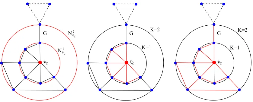
Figure 1: The left-most figure shows the determination ofK-layer centroid expansion subgraphs for a graphG(V, E)
which hold|N1
ˆ
vC|= 6and|N 2 ˆ
vC|= 10vertices. While the middle and the right-most figure show the corresponding1
-layer and2-layer subgraphs regarding the centroid vertexvˆC, and are depicted by red-colored edges. In this example,
the vertices of differentK-layer subgraphs regarding the centroid vertexˆvC are calculated by Eq.(6), and pairwise
vertices possess the same connection information in the original graphG(V, E).
subgraph is the graphG(V, E)itself. An example of the generation of a K-layer subgraph for a
graphG(V, E)is shown in Fig.1.
Definition 2.1 (Centroid-based complexity trace): Let the family of centroid expansion
sub-graphs for G(V, E) be {G1,· · · ,GK,· · · ,GL}. We measure the entropies of the subgraphs and
establish the centroid-based complexity traceDC forG(V, E)as
DBC(G) = {HS(G1),· · ·, HS(GK),· · ·, HS(GL)}, (8)
where· · · , HS(GK)is the Shannon entropy associated with the steady state random walk on the
K-layer centroid expansion subgraphGK. 2
For a graph G(V, E)havingnvertices, computing the centroid depth-based complexity trace
DC(G)ofG(V, E)requires time complexityO(Ln2). This follows the definition in Eq.(7). For
a graphG(V, E), the Dijkstra’s algorithm requires time complexityO(n2). Computing the
Shan-non entropies of theL K-layer centroid expansion subgraphs requires time complexity O(Ln2).
2.3. Theh-Layer Depth-Based Representation of A Graph
In this subsection, we develop the centroid-based complexity trace further by defining a h
-layer depth-based representation around each vertex for a graph (i.e., a depth-based complexity
trace around each vertex). Unlike the centroid-based complexity trace that only reflects the depth
complexity information from the centroid vertex, for all vertices theh-layer depth-based
represen-tations reflect the depth complexity information from any vertex.
For an undirected graph G(V, E) and its shortest path matrix SG, let NvK be a subset of V
satisfying NK
v = {u ∈ V | SG(v, u) ≤ K}. For G(V, E), the K-layer expansion subgraph
GK
v (VvK;EvK)around the vertexv is
VK
v ={u∈NvK};
EK
v ={(u, v)⊂NvK ×NvK |(u, v)∈E}.
(9)
LetLmax be the greatest length of the shortest paths fromv to the remaining vertices ofG(V, E).
IfLv ≥Lmax, theLv-layer expansion subgraph isG(V, E)itself.
Definition 2.2 (h-layer depth-based representation): For a graphG(V, E)and a vertexv ∈ V,
theh-layer depth-based representation around the vertexv ofG(V, E)is ahdimensional vector
DBhG(v) = [HS(G1
v),· · · , HS(G K
v ),· · · , HS(G h v)]
T
(10)
whereh(h≤Lv)is the length of the shortest paths from the vertexv to the remaining vertices in
G(V, E),GvK(VK
v ;EvK) (K ≤h)is theK-layer expansion subgraph ofG(V, E)around the vertex
v, andHS(GK
v )is the Shannon entropy ofGvK defined in Eq.(4). 2
For a graph G(V, E) having n vertices, computing the h-layer depth-based representation
Dh
G(v) of G(V, E) around all vertices v ∈ V requires time complexity O(hn3). This follows
the definition in Eq.(9). For a graph G(V, E), the Dijkstra algorithm requires time complexity
O(n2). Computing the Shannon entropies of theh K-layer expansion subgraphs, which are
de-rived fromv, requires time complexityO(hn2). Hence, the overall time complexity of computing
3. A Jensen-Shannon Subgraph Kernel
In this section, we develop a fast subgraph kernel using the Jensen-Shannon divergence. We
commence by showing how to compute the Jensen-Shannon divergence for (sub)graphs. For a
pair of graphs, we develop the new subgraph kernel by measuring the Jensen-Shannon divergence
between the subgraph entropies from their centroid-based complexity traces.
3.1. A Composite Entropy of Graphs Through The Disjoint Union Graph
To compute the Jensen-Shannon divergence between a pair of graphs, we require a composite
structure for the graphs. In our previous work [4], we have used the product union to construct
the composite graph. Unfortunately, constructing a product graph is computationally burdensome.
Furthermore, the number of vertices for a product graph can be large. Thus, the product graph
will dominate the computation of the Jensen-Shannon divergence. To overcome this problem, we
propose to use a different strategy for constructing a composite structureGp ⊕Gq for a pair of
graphsGp(Vp, Ep)andGq(Vq, Eq). We turn to the disjoint union for constructing our composite
structure. According to [25], the disjoint union graph ofGp(Vp, Ep)andGq(Vq, Eq)is
GDU =Gp∪Gq={Vp∪Vq, Ep∪Eq}. (11)
Through Eq.(11), we observe that the size of the disjoint union graph GDU for Gp(Vp, Ep) and
Gq(Vq, Eq)is|Vp|+|Vq|. By contrast, the size of the product graph forGp(Vp, Ep)andGq(Vq, Eq)
is|Vp||Vq|. In other word, the size of the disjoint union graph for a pair of graphs is much smaller
than their product graph.
Let graphsGp(Vp, Ep)andGq(Vq, Eq)be the connected components of the disjoint union graph
GDU(VDU, EDU), then we compute the relative sizes of the connected components as
ρp = |
V(Gp)|
|V(GDU)|
= |V(Gp)| (|V(Gp)|+|V(Gq)|)
.
and
ρq = |
V(Gq)| |V(GDU)|
= |V(Gq)|
(|V(Gp)|+|V(Gq)|).
The entropy (i.e., the composite entropy) [26] ofGDU is then
Here the entropy functionHS is the Shannon entropyHS(·)defined in Eq.(4).
3.2. A Jensen-Shannon Divergence on Graphs
The classical Jensen-Shannon divergence is a nonextensive mutual information dissimilarity
measure defined on probability distributions. AssumeM+1(χ)is a set of probability distributions
where χ is a set provided with some σ − algebra of measurable subsets, the Jensen-Shannon
divergence DJ S : M+1(χ) × M+1(χ) → R between the probability distributions P and Q, is
negative definite (nd) with the following function [23]:
DJ S(P, Q) = 1
2DKL(P||M) + 1
2DKL(Q||M) = 1
2
Z
χ ln(dP
dM)dP +
1 2
Z
χ
ln(dQ
dM)dQ, (13)
whereM = P+2Q and DKL(P||M) = R
χln( dP
dM)dP is the Kullback-Leibler divergence between
P andM. Ifχis countable, i.e.,P = (p1, p2, . . . , pN)andQ = (q1, q2, . . . , qN)are two discrete
probability distributions, a more general definition is
DJ S(P, Q) =HS(
P +Q
2 )−
HS(P) +HS(Q)
2 , (14)
whereHS(P) =PM
m=1pmlogpm is a Shannon entropy of the probability distributionP. We
de-fined a Jensen-Shannon divergence measure for a pair of graphs. Given a pair of graphsGp(Vp, Eq)
andGq(Vq, Eq), the Jensen-Shannon divergence for them is
DJ S(Gp, Gq) =HS(Gp ⊕Gq)−
HS(Gp) +HS(Gq)
2 . (15)
whereGp⊕Gq is the composite structure formed by the graphsGp(Vp, Eq)andGq(Vq, Eq). Here
we use the disjoint union defined in Sec.3.1 as the composite structure, and the entropy function
HS(·)is the Shannon entropy associated with the steady state random walk defined in Eq.(4).
With the Jesnen-Shannon divergence for graphs defined in Eq.(14) to hand, we define a
Jensen-Shannon diffusion graph kernelkJ S:Gp×Gq →Rwith the kernel value
whereλis a decay factor and satisfies0< λ≤1. Note that, unlike the Jensen-Shannon divergence which is a dissimilarity measure, the Jensen-Shannon diffusion kernel is an information theoretic
similarity measure of a pair of graphs.
Lemma 3.1.The Jensen-Shannon diffusion kernel defined in Eq.(16) is positive definite (pd).
Proof. This follows the definition in [27]. If a similarity or dissimilarity measure sG(Gp, Gq)
between a pair of graphsGpandGqis symmetrical, then a diffusion kernelks = exp(λsG(Gp, Gq))
orks = exp(−λsG(Gp, Gq))associated with the (dis)similarity measuresG(Gp, Gq)ispd.
Note that, a positive definite graph kernel is often called avalid kernel. Clearly, imposing a
graph kernel to be positive definite restricts the broad class of similarity-based graph kernels into
a small group of valid kernels. However, it has been observed that the property of positive
defi-niteness is crucial for the definition of kernel machines and turns out to implicate a considerable
number of theoretical merits associated with graph kernels [28].
For a pair of graphs Gp(Vp, Ep)and Gq(Vq, Eq)each of which has n vertices, computing the
Jensen-Shannon diffusion kernel kJ S(Gp, Gq) in Eq.(16) requiresO(n2) operations. This is
be-cause bothHS(Gp)andHS(Gp)require time complexityO(n2). The disjoint union graph entropy
HS(GDU)can be directly computed based on HS(Gp) and HS(Gp) according to Eq.(12). As a
result, the Jensen-Shannon diffusion kernelkJ S(Gp, Gq)requires time complexityO(n2).
3.3. The Jensen-Shannon Subgraph Kernel
In this subsection, we develop a fast Jensen-Shannon subgraph kernel (kJ S) as an
infor-mation theoretic decomposition kernel. The proposed kernel kJ S is defined by kernelizing the
centroid-based graph complexity traces. This is done by measuring the information content
sim-ilarities for the K-layer subgraphs using the Jensen-Shannon divergence. For a graph G(V, E),
we commence by identifying the centroid vertexvˆC using Eq.(6). Based on ˆvC we construct the
K-layer centroid expansion subgraph GK of G(V, E) using Eq.(7). As we increase K from 1
to the greatest shortest path length L with respect to the centroid vertex vˆC, we obtain a
fam-ily of centroid expansion subgraphs {G1,· · · ,GK,· · · ,GL}. We then measure the entropies of
the subgraphs and establish the depth-based representationDBC(G)of G(V, E)asDBC(G) =
com-pute a similarity measure between their depth-based representationsDBC(Gp)andDBC(Gq)as
follows
s(DBC(Gp), DBC(Gq))= L
X
K=1
sH(H(Gp;K), H(Gq;K)). (17)
wheresH(H(Gp;K), H(Gq;K)) is an entropy-based similarity measure for the K-layer subgraphs
Gp;K and Gq;K of Gp(Vp, Ep) and Gq(Vq, Eq). By using the Jensen-Shannon diffusion kernel
kJ S(·,·)in Eq.(16) as the entropy-based similarity measuresH(·,·)in Eq.(17), the similarity
be-tween the depth-based representationsDBC(Gp)and DBC(Gq)is formulated as the sum of the
diffusion kernel measures for all the pairs ofK-layer subgraphs ofGp(Vp, Ep)andGq(Vq, Eq).
Definition 3.1 (Jensen-Shannon subgraph kernel): Consider a pair of graphs Gp(Vp, Ep) and
Gq(Vq, Eq). The Jensen-Shannon subgraph kernelkJ S(Gp, Gq)is defined as
kJ S(Gp, Gq) = s(DBC(Gp), DBC(Gq))= L
X
K=1
kJ S(Gp;K,Gq;K). (18)
where Gp;K(Vp;K,Ep;K) and Gq;K(Vq;K,Eq;K) are the K-layer centroid expansion subgraphs of
Gp(Vp, Ep)and Gq(Vq, Eq)rooted at their corresponding centroid vertices ˆvp;C andvˆq;C,
respec-tively, andkJ S(Gp;K,Gq;K)is the Jensen-Shannon diffusion kernel between Gp;K(Vp;K,Ep;K)and
Gq;K(Vq;K,Eq;K). According to Eq.(12), Eq.(15) and Eq.(16),kJ S(Gp;K,Gq;K)is
kJ S(Gp;K,Gq;K) = exp{
2|Vp;K| − |Vq;K| 2|Vp;K|+ 2|Vq;K|
λH(Gp;K) +
2|Vq;K| − |Vp;K| 2|Vp;K|+ 2|Vq;K|
λH(Gq;K)}. (19)
Lemma 3.2.The Jensen-Shannon subgraph kernelkJ S ispd.
Proof.For all{c1,· · ·, cN} ⊆Rand anyN graphs{G1,· · · , GN}we have the following
expres-sion
N
X
i,j=1
cicjkJ S(Gi, Gj) = N
X
i,j=1
cicj{ L
X
K=1
kJ S(Gi;K,Gj;K)}
= N
X
i,j=1
cicjkJ S(Gi;1,Gj;1)+, ...,+
N
X
i,j=1
cicjkJ S(Gi;L,Gj;L).
Here for all{c1, ..., cN} ⊆Rand any choice of theN subgraphs{G1;K,· · · ,GN;K}which are the
K-layer centroid expansion subgraphs of theN graphs{G1,· · · , GN}, we have
N
X
i,j=1
sincekJ S ispd(Lemma 3.1). Therefore, we have
N
X
i,j=1
cicjkJ S(Gi, Gj)≥0,
and the proposed Jensen-Shannon subgraph kernel is alsopd.
Note that, for a pair of graphsGp(Vp, Ep)andGq(Vq, Eq)with different sizes, the longest
lay-ers of their expansion subgraphs could be different. Suppose thatvˆC;p and ˆvC;q are the centroid
vertices ofGp(Vp, Ep)andGq(Vq, Eq), and the lengths of the greatest shortest paths from the
cen-troid verticesvˆC;p andˆvC;qareLp andLq, respectively, whereLp > Lq. In practical computations,
to balance the layer difference between the largest centroid expansion subgraphs of the two graphs,
we use the graphGq(Vq, Eq)as the(Lq+ 1)-layer toLp-layer expansion subgraphs ofGq(Vq, Eq).
As a result, for a set of graphs{G1, . . . , Gs, . . . , Gl, . . . , GN}in whichGl has the greatest
short-est path from the centroid vertex, we use each graph Gs itself as the (Ls + 1)-layer to Ll-layer
expansion subgraphs.
3.4. Analysis of Computational Complexity
For a pair of graphs each of which has n vertices andL layer expansion subgraphs, the
pro-posed Jensen-Shannon subgraph kernel requires time complexityO(n2). This is because
comput-ing the centroid-based representations requires time complexityO(Ln2). Computing the
Jensen-Shannon diffusion kernel between the centroid depth-based representations requires time
com-plexityO(L). Lusually tends to be√3
n. As a result, the overall time complexity isO(n2). This
indicates that for a pair of graphs the time complexity of the Jensen-Shannon subgraph kernel
tends to be quadratic in the vertex number of the larger graph. Thus, the new subgraph kernel can
be computed in a polynomial time.
3.5. Discussion
We make three observations regarding the Shannon subgraph kernel. First our
Jensen-Shannon subgraph kernel is equivalent to the similarity measure between depth-based
represen-tations of graphs. Since a depth-based representation of a graphG(V, E)exhibits high dimensional
Our subgraph kernel kJ S captures richer complexity based information than that obtained from
straightforwardly applying the Jensen-Shannon diffusion kernel to the original graphs. Second, the
Jensen-Shannon subgraph kernel only compares pairs of subgraphs with the same layer sizeK.
This avoids enumerating all pairs of subgraphs and renders the computation efficient. Third, for a
pair of graphs, the Jensen-Shannon subgraph kernel can also efficiently measure the similarity of
theirL-layer subgraphs (i.e., the two graphs themselves). Hence, our Jensen-Shannon subgraph
kernel overcomes the subgraph size restriction which commonly arises in existing R-convolution
graph kernels.
4. An Entropic Isomorphism Kernel
In this section, we develop an entropic graph isomorphism kernel. We commence by defining
an entropy-based isomorphism test for a pair ofK-layer expansion subgraphs. Then we develop
the new subgraph kernel by measuring the similarity measure betweenh-layer depth-based
repre-sentations for a pair of graphs using the new isomorphism test.
4.1. An Entropy-Based Isomorphism Test
For a graph G(V, E) and its vertices v and u, GK
v (VvK;EvK) and GuK(VuK;EuK) are the
cor-responding K-layer expansion subgraphs around v and u defined by Eq.(9). We perform the
following isomorphism test onGK
v (VvK;EvK)andGuK(VuK;EuK)as
I(GK v ,G
K u ) =
1 ifHS(GK
v ) =HS(GuK),
|VK
v |=|VuK|, |EvK|=|EuK|, andlv =lu =K,
0 otherwise.
(20)
where if I(GK
v ,GuK) = 1, then GvK ≃ GuK (i.e., GvK andGuK are isomorphic). Here, lv andlu are
respectively the longest shortest path lengths ofGvK andGuK from the verticesv andu.
For a pair of graphs each of which has n vertices, the proposed entropy-based isomorphism
test requests time complexityO(n2). Because the test relies on computing the Shannon entropy
associated with the steady state random walk, it has time complexityO(n2). This indicates that
4.2. The Entropic Isomorphism Kernel
In this subsection, we develop an entropic isomorphism kernel (kh
ISK) using the
entropy-based isomorphism test between the K-layer expansion subgraphs. We commence by
develop-ing a similarity measure between a pair ofh-layer depth-based representations. For a vertexvp
of a graph Gp(Vp, Ep) and a vertex vq of a graph Gq(Vq, Eq), we compute their h-layer
depth-based representations DBhGp(vp) = {HS(G1
v;p),· · · , HS(GvK;p),· · · , HS(Gvh;p)} and DB h
Gq(vq) =
{HS(G1
v;q),· · · , HS(GvK;q),· · · , HS(Gvh;q)} respectively. We compute the similarity measure
be-tween theh-layer depth-based representationsDBhGp(vp)andDBhGq(vq)as
sI(DBhGp(vp), DB
h
Gq(vq))=
h
X
K=1
I(GvK;p,G K
v;q), (21)
whereI(GK
v;p,GvK;q)is the entropy-based isomorphism test defined in Eq.(20).
Definition 4.1 (Entropic Isomorphism kernel): ConsiderGp(Vp, Ep)andGq(Vq, Eq)as a pair of
sample graphs. The entropic isomorphism kernelkISKh using theh-layer depth-based
representa-tions of graphs is defined as
khISK(Gp, Gq) =
X
vp∈Vp X
vq∈Vq
sI(DGhp(vp), D
h Gq(vq))
= X
vp∈Vp X
vq∈Vq
h
X
K=1
I(GK v;p,G
K
v;q). (22)
Intuitively, the entropic isomorphism kernelkISK(h) ispd, because it counts the number of
iso-morphic expansion subgraphs between each pair ofh-layer depth-based representations. In other
words,kISK(h) can be seen as an example of the classical R-convolution graph kernels by counting
the number of isomorphic expansion subgraph pairs.
4.3. Analysis of Computational Complexity
For a pair of graphs each of which has n vertices, the entropic isomorphism kernel requires
time complexityO(n3). This is because computing the h-layer depth-based representations for
the graphs over all vertices requires time complexityO(hn3). Measuring the isomorphism based
The layerhusually tends to be much smaller than n. As a result, the time complexity isO(n3).
This indicates that the entropic isomorphism kernel can also be computed in a polynomial time,
though this kernel may require more time complexity than the Jensen-Shannon subgraph kernel.
4.4. Relationship with the All Subgraph Kernel
In this subsection, we explore the relationship between our entropic isomorphism kernel and
the classical all subgraph kernel. LetGp(Vp, Ep)andGq(Vq, Eq)be two graphs, the all subgraph
kernel [3] is defined as
ksubgraph(Gp, Gq) =
X
Sp⊑Gp X
Sq⊑Gq
δ(Sp, Sq), (23)
where
δ(Sp, Sq) =
1 ifSp ≃Sq, 0 otherwise.
(24)
Here,δis the Dirac kernel, that is, it is1if the arguments are equal and0otherwise (i.e., it is 1 if
a pair of subgraphs are isomorphic and 0 otherwise).
We show the equivalence between the entropic isomorphism kernelkh
ISK and the all subgraph
kernelksubgraph. To this end, we consider a pair of graphs asGp(Vp, Ep)andGq(Vq, Eq). LetGKvp
andGK
vq be the expansion subgraph sets which contain all the K-layer (1 ≤ K ≤ h) expansion
subgraphs around the verticesvp ∈Vpandvp ∈Vqrespectively. Based on the definition in Eq.(20),
for any pair of subgraphsSp(Vp;Ep)andSq(Vq;Eq)we rewrite Eq.(24) as
δ(Kv,u)(Sp, Sq) =
1 if HS(Sp) =HS(Sq),
Sp ∈GKvp, Sq∈G
K vq,
|Vp|=|Vq|, |Ep|=|Eq|, andlvp =lvq =K,
0 otherwise.
(25)
where lvp and lvq are the longest shortest path lengths of Sp and Sq from the vertices vp and vq
random walks on Sp and Sq respectively. Associated with Eq.(25), the kernel kISKh can be
re-defined by re-writing Eq.(23) as
khISK(Gp, Gq) =ksubgraph(Gp, Gq)
= h
X
K=1 X
vp∈Vp X
vq∈Vq X
Sp∈GKvp X
Sq∈GKvq
δ(Kvp,vq)(Sp, Sq). (26)
Through Eq.(23) and Eq.(26), we observe that both the kernels ksubgraph and kISKh need to
identify all pairs of isomorphic subgraphs. Moreover, for the kernelsksubgraphandkISKh each
iso-morphic subgraph pair adds an unit value to the kernel value. Thus, both the entropic isomorphism
kernel and the all subgraph kernel count the number of isomorphic subgraph pairs and thus have
equivalence.
Furthermore, comparing the entropic isomorphism kernel and the all subgraph kernel, we also
observe three differences that conclude the advantage of the entropic isomorphism kernel. a) First,
for the entropic isomorphism kernel we can efficiently measure the isomorphism for a pair of
subgraphs of large size. The reason for this is that the computational complexity of the Shannon
entropy associated with the steady state random walk is quadratic in the (sub)graph size. While for
the all subgraph kernel, measuring the isomorphism between a pair of subgraphs usually requires
burdensome computation. b) Second, the entropic isomorphism kernel overcomes the NP-hard
problem of measuring all pairs of subgraphs that arise in the all subgraph kernel. c) Third, for the
entropic isomorphism kernel, only the pair of expansion subgraphs having the same shortest paths
of greatest lengths around their rooted vertices are evaluated for measuring isomorphism. In other
words, only a pair of expansion subgraphs having the same layers around the rooted vertices can
be evaluated. On the other hand, the all subgraph kernel roughly or arbitrarily evaluates a pair
of subgraphs and counts the isomorphic subgraph pairs. Hence, the entropic isomorphism kernel
also encapsulates location information between pairs of subgraphs, and this is ignored by the all
5. Experimental Results
In this section, we empirically evaluate the performance of our new subgraph kernels. Our
experimental evaluation consists of two parts. First, we test our subgraph kernels on the graph
classification problem using standard graph datasets. These graphs are abstracted from
bioinfor-matics and computer vision databases. Moreover, we also compare our new subgraph kernels with
several state-of-the-art methods. Second, we evaluate the computational efficiency of our new
subgraph kernels.
5.1. Graph Datasets
We demonstrate the performance of our new subgraph kernels on six standard graph based
datasets abstracted from problems formulated by bioinformatics and computer vision. These
datasets include: MUTAG, D&D, ENZYMES, BAR31, BSPHERE31, GEOD31, CATH2, NCI1,
NCI109, COIL5, Shock, PPIs, GATORBait and PTC(MR). More details concerning the datasets
are shown in Table.1.
MUTAG:The MUTAG dataset consists of graphs representing 188 chemical compounds, and here
the goal is to predict whether each compound possesses mutagenicity [33]. The maximum,
mini-mum and average number of vertices are 28, 10 and 17.93 respectively. As the vertices and edges
of each compound are labeled with a real number, we transform these graphs into unweighted
graphs.
D&D:The D&D dataset contains 1178 protein structures [34]. Each protein is represented by a
graph, in which the vertices are amino acids and two vertices are connected by an edge if they are
less than 6 Angstroms apart. The prediction task is to classify the protein structures into enzymes
and non-enzymes. The maximum, minimum and average number of vertices are 5748, 30 and
284.32 respectively.
ENZYMES: The ENZYMES dataset consists of graphs representing protein tertiary structures,
and contains 600 enzymes from the BRENDA enzyme database [37]. In this case, the task is to
correctly assign each enzyme to one of the 6 EC top-level classes. The maximum, minimum and
BAR31, BSPHERE31 and GEOD31:The SHREC 3D Shape database consists of15classes and
20 individuals per class, that is 300 shapes [29]. This is a standard benchmark in 3D shape
recog-nition. From the SHREC 3D Shape database, we establish three graph datasets named BAR31,
BSPHERE31 and GEOD31 datasets through three mapping functions. These functions are a)
ERG barycenter: distance from the center of mass/barycenter, b) ERG bsphere: distance from the
center of the sphere that circumscribes the object, and c) ERG integral geodesic: the average of
the geodesic distances to all other points. Details of the three mapping function can be found in
[29]. The number of maximum, minimum and average vertices for the three datasets are a) 220,
41 and 95.42 (for BAR31), b) 227, 43 and 99.83 (for BSPHERE31), and c) 380, 29 and 57.42 (for
GEOD31), respectively.
CATH2:The CATH2 dataset has proteins in the same class (i.e., Mixed Alpha-Beta), architecture
(i.e., Alpha-Beta Barrel), and topology (i.e., TIM Barrel), but in different homology classes (i.e.,
Aldolase vs. Glycosidases) [2]. The CATH2 dataset is harder to classify, since the proteins in the
same topology class are structurally similar. The protein graphs are10times larger in size than
chemical compounds, with200−300vertices. There is190testing graphs in the CATH2 dataset.
NCI1 and NCI109: The NCI1 and NCI109 datasets consist of graphs representing two balanced
subsets of datasets of chemical compounds screened for activity against non-small cell lung cancer
and ovarian cancer cell lines respectively [35, 36]. There are 4110 and 4127 graphs in NCI1 and
NCI109 respectively.
COIL5: We establish a COIL5 dataset from the COIL database. The COIL image database
con-sists of images of 100 3D objects. We use the images for the first five objects. For each object
we employ 72 images captured from different viewpoints. For each image we first extract corner
points using the Harris detector, and then establish Delaunay graphs based on the corner points
as vertices. As a result, in the dataset there are 5 classes of graphs, and each class has 72 testing
graphs. The number of maximum, minimum and average vertices for the dataset are 241, 72 and
144.90 respectively.
Shock: The Shock dataset consists of graphs from the Shock 2D shape database. Each graph is a
skeletal-based representation of the differential structure of the boundary of a 2D shape. There are
PPIs: The PPIs dataset consists of protein-protein interaction networks (PPIs). The graphs
de-scribe the interaction relationships between histidine kinase in different species of bacteria.
His-tidine kinase is a key protein in the development of signal transduction. If two proteins have
direct (physical) or indirect (functional) association, they are connected by an edge. There are 219
PPIs in this dataset and they are collected from 5 different kinds of bacteria (i.e., a)Aquifex4 and
thermotoga4 PPIs fromAquifex aelicusandThermotoga maritima, b)Gram-Positive52 PPIs from
Staphylococcus aureus, c)Cyanobacteria73 PPIs fromAnabaena variabilis, d)Proteobacteria40
PPIs from Acidovorax avenae, and e) Acidobacteria46 PPIs). Note that, unlike the experiment
in [38] that only uses theProteobacteria40 and theAcidobacteria46 PPIs as the testing graphs, we
use all the PPIs as the testing graphs in this paper. As a result, the experimental results for some
kernels are different on the PPIs dataset.
GatorBait:GatorBait has 100 shapes representing fishes from 30 different classes [29]. We have
extracted Delaunay graphs from their shape quantization (Canny algorithm followed by contour
decimation). Since the classes are associated to fish genus and not to species, we find high
intra-class variability in many cases. Therefore, the database, though having only 100 samples, plays a
challenging role in testing graph classification. The number of maximum, minimum and average
vertices for the dataset are 545, 239 and 348.70.
PTC:The PTC (The Predictive Toxicology Challenge) dataset records the carcinogenicity of
sev-eral hundred chemical compounds for male rats (MR), female rats (FR), male mice (MM) and
female mice (FM) [11]. These graphs are very small (i.e., 20− 30 vertices), and sparse (i.e.,
25−40edges. We select the graphs of male rats (MR) for evaluation. There are344test graphs
in the MR class.
5.2. Experiments on Graph Datasets
We evaluate the performance of our proposed Jensen-Shannon subgraph kernel (JSSK) and
the entropic isomorphism kernel (ISK) on several standard graph datasets, and then compare them
with several alternative state of the art graph kernels. The graph kernels used for comparison
in-clude: 1) the backtraceless random walk kernel using the Ihara zeta function based cycles (BRWK)
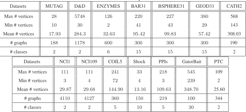
Table 1: Information of the Graph-based Datasets
Datasets MUTAG D&D ENZYMES BAR31 BSPHERE31 GEOD31 CATH2
Max # vertices 28 5748 126 220 227 380 568
Min # vertices 10 30 2 41 43 29 143
Mean # vertices 17.93 284.3 32.63 95.42 99.83 57.42 308.03
# graphs 188 1178 600 300 300 300 190
# classes 2 2 6 15 15 15 2
Datasets NCI1 NCI109 COIL5 Shock PPIs GatorBait PTC
Max # vertices 111 111 241 33 218 545 109
Min # vertices 3 4 72 4 3 239 2
Mean # vertices 29.87 29.68 144.90 13.16 109.63 348.70 25.60
# graphs 4110 4127 360 150 219 100 344
# classes 2 2 5 10 5 30 2
[8], 4) the graphlet count graph kernels with graphlet of size 3(GCGK) [30], 5) the unaligned
quantum Shannon kernel (UQJS) [38], and 6) the attributed graph kernel from the
Jensen-Tsallis q-differences associated withq = 2(JTQK) [39]. For our ISK kernel, we set the largest
value of h as 10, i.e., at most 10 expansion subgraphs around a vertex are considered. For the
WL kernel and JTQK kernel, we set the largest iteration of the required vertex label
strengthen-ing methods (i.e., the WL algorithm for the WL subtree kernel and the tree-index method for the
JTQK kernel) as 10.
For each kernel, we compute the kernel matrix on each graph dataset. We perform 10-fold
cross-validation using the C-Support Vector Machine (C-SVM) Classification, and compute the
classification accuracies, using LIBSVM. We use nine samples for training and one for testing.
The C-SVMs classification was performed with its parameters optimized on each dataset. We
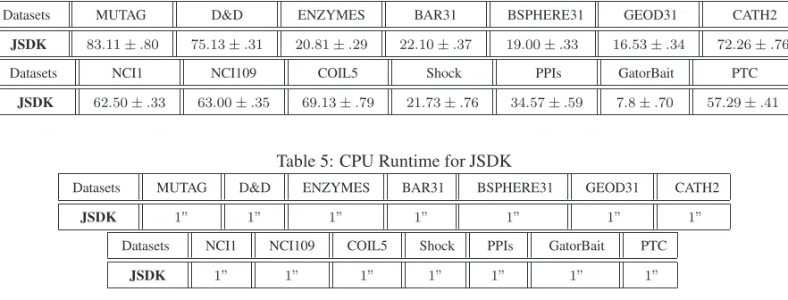
report the average classification accuracies and standard errors from the10-fold cross-validation
for each kernel in Table.2. Furthermore, we also report the runtime of computing the kernel
matrices for each kernel in Table.3. Here, the runtime was measured under Matlab R2011a running
on a2.5GHz Intel2-Core processor (i.e., i5-3210m). Finally, note that, the JTQK, WL and SPGK
kernels are able to accommodate attributed graphs. In our experiments, we use the vertex degree
(not the original vertex labels) as the vertex label for the JTQK, WL and SPGK kernels. Thus,
Table 2: Classification Accuracy (In%±Standard Error) Comparisons
Datasets MUTAG D&D ENZYMES BAR31 BSPHERE31 GEOD31 CATH2
JSSK 83.77±.74 76.32±.46 24.38±.55 52.76±.47 43.33±.40 32.03±1.02 75.42±.76
ISK 84.66±.56 75.32±.35 41.80±.43 62.80±.47 52.50±47 39.76±.43 67.55±.67 JTQK 83.22±.87 74.35±.23 39.38±.76 60.56±.35 46.93±.61 40.10±.46 68.70±.69
UQJS 82.72±.44 −− 36.58±.46 30.80±.61 24.80±.61 23.73±.66 71.11±.88
BRWK 77.50±.75 −− 20.56±.35 −− −− −− −−
WL 82.05±.57 73.52±.20 38.41±.45 58.53±.53 42.10±.68 38.20±.68 67.36±.63
SPGK 83.38±.81 −− 28.55±.42 55.73±.44 48.20±.76 38.40±.65 81.89±.63 GCGK 82.04±.39 74.70±.30 24.87±.22 22.96±.65 17.10±.60 15.30±.68 73.68±1.09
Datasets NCI1 NI109 COIL5 Shock PPIs GatorBait PTC
JSSK 64.86±.24 65.72±.26 67.75±.67 37.66±.80 45.04±.80 9.20±.65 56.94±.43
ISK 76.21±.25 76.42±.24 38.30±.56 39.86±.68 79.47±.32 11.40±.52 60.26±.42 JTQK 81.23±.25 81.40±.26 30.86±.66 37.73±.72 88.47±.47 9.60±.87 57.47±.41 UQJS 69.09±.20 70.17±.23 70.11±.61 40.60±.92 65.61±.77 9.00±.89 56.70±.49
BRWK 60.34±.17 59.89±.15 14.63±.21 0.33±.37 −− −− 53.97±.31
WL 80.68±.27 80.72±.29 33.16±1.01 36.40±1.00 88.09±.41 10.10±.61 56.85±.52 SPGK 74.21±.30 73.89±.28 69.66±.52 37.88±.93 59.04±.44 9.00±.75 55.52±.46 GCGK 63.72±.12 62.33±.13 66.41±.63 26.93±.63 46.61±.47 8.40±.83 55.41±.59
D&D, ENZYMES, PTC datasets that have original label information residing on vertices) may be
different from those reported in [5, 8, 39].
Experimental Results: a) On the MUTAG dataset, the accuracy of our ISK kernel exceeds the
alternative kernels. The accuracy of our JSSK kernel is competitive to that of the ISK kernel,
but exceeds other kernels. b) On the D&D dataset, the accuracy of our JSSK kernel exceeds the
alternative kernels. The accuracy of our ISK kernel is competitive to that of the JSSK and WL
kernels, and exceeds other kernels. The SPGK and BRWK kernels cannot complete the required
computations on the D&D dataset, because the graphs in the dataset are very large (e.g., some
graphs have more than thousands vertices). c) On the ENZYMES, BAR31, BSPHERE31 and
GEOD31 datasets, the accuracies of our ISK kernel obviously exceed those of the remaining
kernels. The classification accuracies of our JSSK kernel are lower than those of the ISK, SPGK
and WL kernels, and exceed other kernels. The BRWK cannot finish the computation on the
BAR31, BSPHERE31 and GEOD31 datasets. This is because the BRWK kernel relies on the
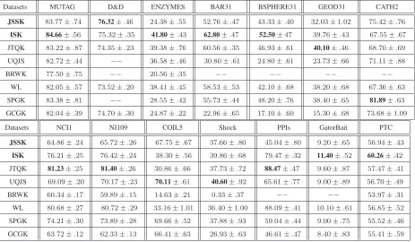
Table 3: CPU Runtime Comparisons
Datasets MUTAG D&D ENZYMES BAR31 BSPHERE31 GEOD31 CATH2
JSSK 1” 45” 1” 1” 1” 1” 4”
ISK 15” 3h28” 3′30” 3′50” 3′10” 2′40” 9′51”
JTQK 3” 23h39′ 30” 1′22” 1′35” 1′17” 39′14”
UQJS 20” >1day 4′23” 10′30” 13′48” 8′49” 1h14′
BRWK 1” >1day 13” −− −− −− >1day
WL 3” 7′43” 21” 30” 25” 15” 53”
SPGK 1” >1day 2” 11” 14” 11” 4′13”
GCGK 1” 1′17” 2” 2” 2” 2” 8”
Datasets NCI1 NCI109 COIL5 Shock PPIs GatorBait PTC
JSSK 52” 53” 3” 1” 2” 3” 4”
ISK 2h19′ 2h20” 9′55” 6” 1′40” 7” 59”
JTQK 10′50” 10′55” 7′19” 3” 1′43” 29′31” 8”
UQJS 2h55′ 2h55′ 18′20” 14” 3′24” 20′53” 1′46”
BRWK 6′49” 6′49” 16′46” 8” >1day >1day 29”
WL 2′31” 2′37” 1′5” 3” 20” 33” 9”
SPGK 16” 16” 31” 1” 22” 2′25” 1”
GCGK 5” 5” 4” 1” 4” 3” 1”
BRWK cannot capture any cycle in these datasets. d) On the CATH2 dataset, the accuracy of the
SPGK kernel exceeds that of the remaining kernels. The accuracy of our JSSK kernel exceeds that
of any kernel, excluding the SPGK kernel. Moreover, the accuracy of the ISK kernel exceeds that
of all the remaining kernels with the exception of the JSSK, JTQK, UQJS and SPGK kernels. e)
Overall, on the NCI1, NCI109, and PPIs datasets, the accuracies of the ISK kernel are only lower
than those of the JTQK and WL kernels, but outperform the remaining kernels. On the other hand,
the JSSK kernel only outperforms the GCGK and BRWK kernels. f) On the GatorBait and PTC
datasets, the accuracies of our ISK kernel exceed those of all the alternative kernels. On the other
hand, the accuracies of our JSSK kernel exceed or are competitive to those of all the alternative
kernels. g) On the Shock dataset, the accuracy of our ISK kernel is only a little lower than that of
the UQJS kernel, and exceeds that of all the remaining kernels. The accuracy of our JSSK kernel
exceeds or is competitive to that of all alternative kernels. h) Finally, on the COIL5 dataset, the
accuracy of our JSSK kernel exceeds or is competitive to that of all the alternative kernels, while
lower than that of all the remaining kernels.
Discussion and Analysis: In terms of the runtime, it is clear that our JSSK kernel is the fastest
kernel. It can efficiently finish the computation on all datasets. The reasons for this efficiency
are twofold. First, for the JSSK kernel the required centroid depth-based representation (i.e.,
the centroid-based complexity trace) of a graph only encapsulates a small number of centroid
expansion subgraphs. In other words, the JSSK kernel only measures limited number of subgraphs.
Second, the associated Jensen-Shannon divergence measure between a pair of centroid expansion
subgraphs only requires computation of quadratic vertex number, even a pair of large global graphs
being compared. On the other hand, for our ISK kernel the efficiency is slower than that of the
JSSK kernel. The reason for this is that the ISK kernel considers the depth-based representations
(i.e., theh-layer depth-based representation around each vertex) rooted from all the vertices. By
contrast, the JSSK kernel only considers the depth-based representation derived from the centroid
vertex. As a result, the ISK kernel needs to measure more expansion subgraphs. Moreover, the
efficiency of the ISK kernel is also slower than the JTQK, UQJS, SPGK, WL and GCGK kernels
on some datasets, but it can still finish the computation in polynomial time. Unlike some kernels
(i.e., the SPGK and BRWK kernels) which can only finish the computation on datasets having
small graphs, our ISK kernel can also finish the computation on datasets having large graphs in
polynomial time. The reason for this is that the required Shannon entropy associated with the
steady state random walk for the ISK kernel can be efficiently computed (i.e., the computation is
quadratic vertex number). As a result, the required h-layer depth-based representations and the
entropy-based isomorphism test can be efficiently computed and measured, respectively.
In terms of the classification accuracies, our ISK kernel outperforms all the alternative kernels
on the MUTAG, ENZYMES, BAR31, BSPHERE31, GatorBait and PTC datasets. On the other
hand, on the PPIs, NCI1 and NCI109 datasets, the accuracies of our ISK kernel are only lower
than those of the JTQK and WL kernels, but are higher than those of other kernels. On the Shock
dataset, the accuracy of our ISK kernel is only a little lower than that of the UQJS kernel, but is
higher than that of other kernels. On the D&D dataset, the accuracy of our ISK kernel is only a
little lower than that of our JSSK kernel, but is higher than that of other kernels. The reason for this