On the effectiveness of cache partitioning in hard real-time systems

systems

.

White Rose Research Online URL for this paper:

http://eprints.whiterose.ac.uk/93504/

Version: Published Version

Article:

Altmeyer, Sebastian, Douma, Roeland, Lunniss, William Richard Elgon et al. (1 more

author) (2016) On the effectiveness of cache partitioning in hard real-time systems.

Real-Time Systems. ISSN 1573-1383

https://doi.org/10.1007/s11241-015-9246-8

[email protected] https://eprints.whiterose.ac.uk/

Reuse

Items deposited in White Rose Research Online are protected by copyright, with all rights reserved unless indicated otherwise. They may be downloaded and/or printed for private study, or other acts as permitted by national copyright laws. The publisher or other rights holders may allow further reproduction and re-use of the full text version. This is indicated by the licence information on the White Rose Research Online record for the item.

Takedown

If you consider content in White Rose Research Online to be in breach of UK law, please notify us by

DOI 10.1007/s11241-015-9246-8

On the effectiveness of cache partitioning in hard

real-time systems

Sebastian Altmeyer1 · Roeland Douma1 ·

Will Lunniss2 · Robert I. Davis2

© The Author(s) 2015. This article is published with open access at Springerlink.com

Abstract In hard real-time systems, cache partitioning is often suggested as a means

of increasing the predictability of caches in pre-emptively scheduled systems: when a task is assigned its own cache partition, inter-task cache eviction is avoided, and timing verification is reduced to the standard worst-case execution time analysis used in non-pre-emptive systems. The downside of cache partitioning is the potential increase in execution times. In this paper, we evaluate cache partitioning for hard real-time systems in terms of overall schedulability. To this end, we examine the sensitivity of (i) task execution times and (ii) pre-emption costs to the size of the cache partition allocated and present a cache partitioning algorithm that is optimal with respect to taskset schedulability. We also devise an alternative algorithm which primarily optimises schedulability but also minimises processor utilization. We evaluate the performance of cache partitioning compared to state-of-the-art pre-emption cost analysis based on benchmark code and on a large number of synthetic tasksets with both fixed priority and EDF scheduling. This allows us to derive general conclusions about the usability of cache partitioning and identify taskset and system parameters that influence the relative effectiveness of cache partitioning. We also examine the improvement in processor

B

[email protected]; [email protected]

Roeland Douma [email protected]

Will Lunniss [email protected]

Robert I. Davis [email protected]

1 _{University of Amsterdam, Amsterdam, The Netherlands}

utilization obtained using an alternative cache partitioning algorithm, and the tradeoff in terms of increased analysis time.

Keywords Timing verification·Cache partitioning·WCET analysis·Real-time

scheduling

Extended version

This paper builds upon and extends the ECRTS 2014 paper onEvaluation of Cache

Partitioning for Hard Real-Time Systems(Altmeyer et al.2014) as follows:

– The evaluation now covers both fixed priority and EDF scheduling.

– We examined how the schedulability of a group of tasks sharing a partition depends upon partition size.

– We present an alternative cache partitioning algorithm which both optimises schedu-lability and minimises processor utilization. We examine the improvement in processor utilization obtained using this algorithm as compared to the original cache partitioning algorithm, and the tradeoff in terms of increased analysis time.

1 Introduction

Cache partitioning is often suggested as a means of increasing the predictability of caches in pre-emptively scheduled hard real-time systems. The rationale behind this argument is that when a task is assigned its own cache partition, inter-task cache evic-tion is avoided, and timing verificaevic-tion is reduced to the standard worst-case execuevic-tion time (WCET) analysis used in non-pre-emptive systems. Cache partitioning comes at a cost. The reduced amount of cache available to each task potentially increases intra-task cache conflicts, trading an increase in (non-pre-emptive) execution times for reduced cache related pre-emption delays (CRPD).

Despite the wealth of publications on cache partitioning for real-time systems, little work has been done on the effectiveness of cache partitioning compared to systems where tasks make unconstrained use of the cache. Pre-emptive multi-tasking systems with unconstrained caches were considered unpredictable. Given recent advances in the analysis of cache related pre-emption delays, we consider this view outdated.

In this paper, we evaluate cache partitioning for hard real-time systems in terms of overall schedulability. To this end, we first determine the sensitivity of task execution times to the size of the available cache partition using application code from real-time benchmarks. Contrary to the implicit assumptions in prior work, the worst-case exe-cution time of a task is not necessarily monotonic in the partition size. We show how the monotonicity property can be re-established using a monotonic upper bound func-tion for the execufunc-tion times. We then present a cache partifunc-tioning algorithm that aims at optimizing taskset schedulability. Under the assumption of monotonic execution times, the algorithm is optimal in the sense that it finds a schedulable cache parti-tioning whenever one exists. The algorithm is based on a branch-and-bound approach and is agnostic with respect to the schedulability test used, i.e., it is valid for any,

sustainableschedulability test (Baruah and Burns2006) and scheduling algorithm.

schedulability as its primary concern and minimizes processor utilization as a sec-ondary concern. This algorithm is optimal under the same conditions, in the sense that it finds a schedulable cache partitioning with the minimum processor utilization whenever a schedulable partitioning exists.

We evaluate the performance of cache partitioning vs. a non-partitioned cache, using state-of-the-art pre-emption cost aware schedulability analysis, based on two different benchmark sets (PapaBench and Mälardalen Benchmark Suite) and on a large number of synthetic tasksets. The evaluation using synthetic tasksets enables us to derive results that are valid in general, and not just for a small selection of use-cases. In addition, we identify how different parameter settings affect the relative performance of the partitioned vs. non-partitioned approaches. We also evaluate the improvement in processor utilization obtained using the alternative cache partitioning algorithm as compared to the original cache partitioning algorithm, and the tradeoff in terms of increased analysis time. Finally, we quantify the error margin introduced by the assumption of monotonic execution times.

We focus on a completely analytical approach, where we compare the schedulability of real-time systems assuming pre-emptive scheduling under either a fixed priority or EDF scheduling policy, with a direct mapped cache. In both cases, partitioned and non-partitioned cache, we rely on bounds on the execution times obtained via WCET analysis, and in the non-partitioned case, also on analytical bounds on the CRPD.

The paper is structured as follows: In Sect.2, we introduce the required terminology and notation and in Sect.3we present the schedulability tests for fixed priority and EDF scheduling. In Sect.4, we review existing approaches to cache partitioning. Section5 explains the sensitivity of the worst-case execution times of tasks with respect to the size of their allocated cache partitions. The optimal cache partitioning algorithms are presented in Sect.6, the results of the case study in Sect.7and the evaluation based on synthetic tasksets in Sect.8. Section9concludes with a summary and discussion of future work.

2 System model, terminology and notation

We consider both fixed priority pre-emptive scheduling and EDF (pre-emptive) scheduling of a set of sporadic tasks (or taskset) on a single processor. Each taskset

Ŵcomprisesn tasksŴ = {τ1, . . . , τn}, wheren is a positive integer. We assume a discrete time model, where all task parameters are positive integers.

Each taskτiis characterized by its bounded worst-case execution timeCi obtained assuming no pre-emption (i.e. not including any cache related pre-emption delays), minimum inter-arrival time orperiod Ti, and relativedeadline Di. Each taskτi there-fore gives rise to a potentially unbounded sequence of invocations orjobs, each of which has an execution time upper bounded byCi, an arrival time at leastTi after the arrival of its previous job, and an absolute deadline that is Di after its arrival. In an

implicit-deadlinetaskset, all tasks haveDi = Ti, in aconstrained-deadlinetaskset,

by accessing mutually exclusive shared resources, with the exception of the proces-sor. (We note that this restriction is only made to simplify comparisons between the different approaches, resource sharing can be accounted for by schedulability analysis that incorporates CRPD as shown by Altmeyer et al.2011,2012).

The utilizationUi, of a task is given by its execution time divided by its period (Ui =Ci/Ti). The total utilizationU of a taskset is the sum of the utilizations of all of its tasks, i.e.

U =

i

Ci/Ti. (1)

2.1 Static timing analysis

The paper is set in the context of static timing analysis as used for many safety-critical hard real-time applications. This means that we derive the worst-case execution timeCi of each taskτi using a static analysis, in our case, the aiT Timing analyzer (Ferdinand and Heckmann2004).

Static timing analyses offer higher reliability compared to measurement-based approaches, as exhaustive measurements are considered infeasible for modern archi-tectures. The higher confidence in the correctness of the execution time estimates comes at the cost of system restrictions, which must be fulfilled in order to apply static timing analyses. Foremost the restriction to static instead of dynamic memory allocation and write-through data caches.

2.2 Pre-emption costs

We now extend the sporadic task model to include pre-emption costs. To this end, we need to explain how pre-emption costs can be derived. To simplify the following explanation and examples, we assume direct-mapped caches.

The additional execution time due to pre-emption is mainly caused by cache evic-tion: the pre-empting task evicts cache blocks of the pre-empted task that have to be reloaded after the pre-empted task resumes. The additional context switch costs due to the scheduler invocation and a possible pipeline-flush can be upper-bounded by a constant. We assume that theseconstant costs are already included inCi. Hence, from here on, we usepre-emption costto refer only to the cost of additional cache reloads due to pre-emption. This cache-related pre-emption delay (CRPD) is bounded byg×BRT wheregis an upper bound on the number of cache block reloads due to pre-emption and BRT is an upper-bound on the time necessary to reload a memory block in the cache (block reload time).

due to a pre-emption atP. The maximum possible pre-emption cost for a task is determined by the program point with the highest number of UCBs. Note that for each subsequent pre-emption, the program point with the next smaller number of UCBs can be considered. Thus, the j-th highest number of UCBs can be counted for the

j-th pre-emption. A tighter definition is presented by Altmeyer and Burguière2009; however, in this paper we need only the basic concept.

The worst-case impact of a pre-empting task is given by the number of cache blocks that the task may evict during its execution. Recall that we consider direct-mapped caches: in this case, loading one block into the cache may result in the eviction of at most one cache block. A memory block accessed during the execution of a pre-empting task is referred to as an evicting cache block (ECB). Accessing an ECB may evict a cache block of a pre-empted task.

In this paper, we represent the sets of ECBs and UCBs as sets of integers with the following meaning:

s∈UCBi ⇔τi has a useful cache block in cache-sets

s∈ECBi ⇔τi may evict a cache block in cache-sets

Separate computation of the pre-emption cost is restricted to architectures without timing anomalies (Lundqvist and Stenström1999) but is independent of the type of cache used, i.e. data, instruction or unified cache.

In the case of set-associative LRU caches1, a single cache-set may contain several useful cache blocks. For instance, UCB1= {1,2,2,2,3,4}means that taskτ1contains 3 UCBs in cache-set 2 and one UCB in each of the cache sets 1,3 and 4. As one ECB suffices to evict all UCBs of the same cache-set (Burguière et al. 2009), multiple accesses to the same set by the pre-empting task does not need to appear in the set of ECBs. Hence, we keep the set of ECBs as used for direct-mapped caches. A bound on the CRPD in the case of LRU caches due to taskτi directly pre-emptingτj is thus given by the intersection UCBj ∩′ ECBi = {m|m ∈ UCBj : m ∈ ECBi}, where the result is also a multiset that contains each element from UCBj if it is also in ECBi. A precise computation of the CRPD in the case of LRU caches is given by Altmeyer et al. (2010). In this paper, we assume direct-mapped caches. Note that all equations provided within this paper are for direct-mapped caches, they are also valid for set-associative LRU caches with the above adaptation to the set-intersection.

3 Schedulability tests

In this section, we present schedulability tests for fixed-priority scheduling using response time analysis and for EDF scheduling using processor demand analysis. Both analyses aresustainable(Baruah and Burns2006) in the sense that any taskset that was deemed schedulable by the test remains schedulable if the parameters “improve”, e.g., if the execution times decrease or periods increase.

3.1 Fixed priority pre-emptive scheduling

We now recapitulate the exact (sufficient and necessary) schedulability test for fixed priority pre-emptive scheduling of constrained-deadline tasksets based on response

time analysis (Audsley et al. 1993; Joseph and Pandya 1986; Davis et al. 2008).

Subsequent work on integrating cache related pre-emption delays into schedulability analysis for fixed priority pre-emptive systems is based on this analysis. The basic form given below assumes that pre-emption costs are zero.

We assume that the indexiof taskτirepresents its priority, henceτ1has the highest priority, andτn the lowest. We use the notation hp(i)(andl p(i)) to mean the set of tasks with priorities higher than (and lower than)i, and the notationhep(i)(and

lep(i)) to mean the set of tasks with priorities higher than or equal to (lower than or

equal to)i.

The worst-case response timeRi of a taskτi is given by the longest possible time from release of a job of the task until it completes execution. Thus taskτiis schedulable if and only ifRi ≤ Di , and a taskset is schedulable if and only if all of its tasks are schedulable.

The response time Ri of a task necessarily contains its execution timeCi, and in addition,τi may suffer interference and be pre-empted by tasks with higher priority thani. Letτj be such a task. Within the response time Ri ofτi, taskτj executes at most

Ri

Tj

times, each time for at mostCj. Hence, the response timeRi of taskτi is given by:

Ri =Ci+

∀j∈hp(i)

Ri

Tj

Cj (2)

where hp(i)denotes the set of tasks with higher priority thani. The response time

Riof taskτi appears on both the left-hand side and the right-hand side of (2). As the right-hand side is a monotonically non-decreasing function ofRi, then a solution may be found via fixed-point iteration:

R_ix+1=Ci+

∀j∈hp(i)

_Rx i

Tj

Cj (3)

Iteration starts with an initial value, typicallyR0_i =Ci, and ends when eitherRix+1>

Di in which case the task is unschedulable, or whenR_ix+1 = R_ix, in which case the task is schedulable, with a worst-case response timeR_ix+1. We note that convergence may be speeded up using the techniques described by Davis et al. (2008).

3.1.1 Pre-emption cost aware schedulability test

Ri =Ci+

∀j∈hp(i)

Ri

Tj

(Cj+γi,j) (4)

An alternative approach was taken by Petters and Farber (2001) and later Staschulat et al. (2005), who based their analyses on the following equation:

Ri =Ci+

∀j∈hp(i)

Ri

Tj

Cj+ ˆγi,j

(5)

The valueγˆi,j denotes the pre-emption cost ofalljobs of taskτj executing during the response time of taskτi (again with j ∈hp(i)). It is given by the

Ri

Tj

-highest pre-emption costs of a job of taskτj executing duringRi. Although the difference with respect to (4) is subtle, more precise analysis can be obtained by usingγˆi,j as a bound on theoverall impactof all jobs ofτj on the response timeRi instead of a bound on the impact ofjust onejob ofτj.

We note that when pre-emption costs are considered explicitly, the worst-case sce-nario is not necessarily given by a synchronous release of all higher priority tasks (Meumeu Yomsi and Sorel2007) and hence (4) and (5) provide sufficient, but not exact schedulability tests.

3.1.2 Pre-emption cost computation

The valueγi,jcan be computed in a number of different ways, which are described in detail by Altmeyer et al. (2012), here, we restrict our explanations to the two dominant approaches: ECB-Union and UCB-Union.

UCB-UnionTan and Mooney (2007) analysed the pre-emption cost via an upper

bound on the number of useful cache blocks (of all empted tasks) that a pre-empting taskτj may evict. As it is only the eviction of useful cache blocks belonging to tasks with equal or higher priority than taskτi that may increase the response time of taskτi, only tasks with intermediate priorities in the set aff(i,j)=hep(i)∩l p(j), need be considered.

γ_iUCB_,j −U=BRT·

⎛ ⎝

k∈aff(i,j)

UCBk

⎞

⎠∩ECBj (6)

Here,γ_iUCB_,j −Urepresents the worst-case impact a job of taskτjcan have on all (useful cache blocks of) tasks with lower priority than taskτjdown to taskτi. We refer to this approach as UCB-Union.

ECB-UnionInstead of considering the precise set of ECBs of a pre-empting task and

by the union of the ECBs of all tasks with higher or equal priority than taskτj:

γ_iECB_,j −U= max

∀k∈aff(i,j)

⎧ ⎨ ⎩ UCBk∩ ⎛ ⎝

h∈hep(j)

ECBh ⎞ ⎠ ⎫ ⎬ ⎭ (7)

The UCB-Union and ECB-Union approaches areincomparablein that there are tasks that may be deemed schedulable using one approach but not the other and vice-versa.

Multiset approachesThe UCB-Union and ECB-Union can be lifted to the so-called

Multiset approaches to be used within Eq. (5) to account for theRi

Tj

-highest pre-emption costs of a job of taskτj executing during Ri instead of accounting for the highest pre-emption costs of a job

Ri

Tj

times. To simplify our equations, we introduce

Ek(Ri)to denote the maximum number of jobs of taskτk that can execute during response timeRi, i.e.:

Ek(Ri)=

_R

i

Tk

The pre-emption costγ_iECB_,j −M is then computed as follows, recognising the fact that taskτjcan pre-empt each intermediate taskτkat mostEj(Rk)Ek(Ri)times during the response time of taskτi. We form a multisetMthat contains the cost

UCBk∩

⎛ ⎝

h∈hp(j)∪{j}

ECBh

⎞

⎠ (8)

ofτjpre-empting taskτk Ej(Rk)Ek(Ri)times, for each taskτk ∈aff(i,j). Hence:

M =

k∈aff(i,j)

⎛ ⎝

Ej(Rk)Ek(Ri)

UCBk∩

⎛ ⎝

h∈hp(j)∪{j}

ECBh

⎞ ⎠

⎞

⎠ (9)

γ_iECB_,j −Mis then given by theEj(Ri)largest values in M.

γ_iECB_,j −M=BRT·

Ej(Ri)

l=1

|Ml| (10)

whereMlis thel-th largest value inM. We note that by construction, the ECB-Union Multiset approach dominates the ECB-Union approach.

The pre-emption costγ_iUCB_,j −Mis computed as follows, recognising the fact that task

τjcan pre-empt each intermediate taskτkdirectly or indirectly at mostEj(Rk)Ek(Ri) times during the response time of taskτi. First, we form a multi-setMiucb,j containing

the fact that during the response timeRiof taskτi, taskτjcannot evict a UCB of task

τkmore thanEj(Rk)Ek(Ri)times. Hence:

M_iucb_,j =

k∈aff(i,j)

⎛ ⎝

Ej(Rk)Ek(Ri)

UCBk

⎞

⎠ (11)

Next, we form a multi-setMecb_j containing Ej(Ri)copies of the ECBj of taskτj . This multi-set reflects the fact that during the response timeRi of taskτi, taskτjcan evict ECBs in the set ECBj at mostEj(Ri)times.

Mecb_j =

Ej(Ri)

(ECBj) (12)

γ_iUCB_,j −Mis then given by the size of the multi-set intersection ofMecb_j andM_iucb_,j

γ_iUCB_,j −M=BRT· M_iucb_,j ∩Mecb_j (13)

We note that by construction, the Union Multiset approach dominates the UCB-Union approach.

The UCB-Union Multiset and the ECB-Union Multiset approach areincomparable

in that there are tasks that may be deemed schedulable using one approach but not the other and vice-versa. More precise analysis can therefore be achieved by using a combination of both approaches as follows:

Ri =min

R_iECB−M,R_iUCB−M (14)

A detailed description of the pre-emption cost aware schedulability tests can be found in Altmeyer et al. (2012).

3.2 EDF scheduling

We now recapitulate the exact (sufficient and necessary) schedulability test for pre-emptive EDF scheduling of sporadic tasksets based onprocessor demand analysis

(Baruah et al.1990). Subsequent work on integrating cache related pre-emption delays into schedulability analysis for EDF scheduled systems is based on this analysis. The basic form given below assumes that pre-emption costs are zero. Pre-emptive EDF scheduling is optimal among all scheduling algorithms on a uniprocessor (Dertouzos 1974) under the assumption of negligible pre-emption overhead.

A necessary and sufficient schedulability test for EDF and implicit deadlines

(Di = Ti) is given by the processor utilizations (Liu and Layland1973): a task set is schedulable, iff

U =

i

Ci

Ti

This test is necessary, but not sufficient ifDi =Ti.

Baruah et al. (1990) introduced the processor demand functionh(t), which denotes the maximum execution time requirement of all tasks jobs which have both their arrival times and their deadlines in a contiguous interval of lengtht. Using this they showed that a taskset is schedulable iff∀t>0,h(t)≤twhereh(t)is defined as:

h(t)=

i=1 max

0,1+

t−Di

Ti

Ci (16)

Ash(t)can only change whentis equal to an absolute deadline, we can restrict the number of values oftthat need to be checked. To place an upper bound ont, and so on the number of calculations ofh(t), the minimum interval in which it can be guaranteed that an unschedulable taskset will be shown to be unschedulable must be found. For a general taskset with arbitrary deadlinestcan be bounded byLa(George et al.1996):

La=max

Di, . . . ,Dn,

n

i+1(Ti =Di)Ui 1−U

(17)

And an alternative bound,Lbgiven by the length of the synchronous busy period can be used (Ripoll et al.1996), whereLbis computed using the following equation using fixed point iteration:

wα+1=

n

i=1

wα

Ti

Ci (18)

There is no direct relationship betweenLa andLb, which enablest to be bounded byL =min(La,Lb). Combined with the knowledge thath(t)can only change at an absolute deadline, a taskset is therefore schedulable under EDF iffU ≤1 and:

∀t∈ Q,h(t)≤t (19)

WhereQis defined as

Q= {dk|dk=kTi+Di∧dk<min(La,Lb),k∈N} (20)

Zhang andBurns (2009) presented the Quick convergence Processor-demand Analysis (QPA) algorithm which exploits the monotonicity ofh(t)to reduce the number of required checks.

3.2.1 Pre-emption cost aware schedulability test

scheduling,γt,j refers to the pre-empting taskτj andt, rather than the pre-empting and pre-empted tasks. Includingγt,j in (16) a revised equation forh(t)is obtained:

h(t)=

i=1 max

0,1+

t−Di

Ti

(Ci+γt,j) (21)

The set of affected tasks for EDF is based on the relative deadlines of the tasks:

aff(tj)= {∀τi|t ≥Di >Dj} (22)

Taskτjcan only pre-empt tasks with a larger relative deadline thanDj and only tasks with a relative deadline Di less than or equal to t need to be accounted for when calculatingh(t)

3.2.2 Pre-emption cost computation

The UCB-Union (see Eq. (23)) and ECB-Union (see Eq. (24)) approaches as used for fixed-priorities can be adapted as follows:

γ_tUCB_,j −U =BRT·

⎛ ⎝

k∈aff(t,j)

UCBk

⎞

⎠∩ECBj (23)

and

γ_tECB_,j −U= max

∀k∈aff(t,j)

⎧ ⎨ ⎩ UCBk∩ ⎛ ⎝

h∈hep(j)

ECBh ⎞ ⎠ ⎫ ⎬ ⎭ (24)

The UCB-Union and ECB-Union approaches areincomparablein that there are tasks that may be deemed schedulable using one approach but not the other and vice-versa. Similar to Eq. (5) that accounts for the highestnpre-emption costs of a job instead of the highest pre-emption costs of a jobntimes, we can adapt Eq. (21) as follows

h(t)=

i=1

max

0,1+

t−Di

Ti

Ci+γt,j

(25)

and lift the UCB-Union and ECB-Union approaches to their multiset counterparts. The ECB-Union multiset approach computes the union of all ECBs that may affect a pre-empted task during a pre-emption by taskτj. It accounts for nested pre-emptions by assuming that task τj has already been pre-empted by all other tasks that may pre-empt it. The first step is to form a multisetMt,j that contains the cost of taskτj pre-empting taskτkrepeatedPj(Dk)Ek(t)times, for each taskτk ∈aff(t,j), where

Pj(Dk)denotes the maximum number of jobs of taskτj that can pre-empt a single job of taskτk:

Pj(Dk)=max

0,

_D

k−Dj

Tj

andEk(t)is defined as

Ek(t)=max

0,

_t

−Dk

Tk

Hence:

M =

k∈aff(t,j)

⎛ ⎝

Pj(Dk)Ek(t)

UCBk∩

⎛ ⎝

h∈hp(j)∪{j}

ECBh

⎞ ⎠

⎞

⎠ (26)

γ_tECB_,j −Mis then given by theEj(t)largest values in M.

γ_tECB_,j −M=BRT·

Ej(t)

l=1

|Ml| (27)

The pre-emption costγ_tUCB_,j −M for EDF scheduling is computed similarly to the UCB-Union Multiset approach for fixed-priority scheduling: Task τj can pre-empt each intermediate taskτk directly or indirectly at mostPj(Dk)Ek(t)times within the deadline of taskτi. First, we form a multi-set Mtucb,j containing Pj(Dk)Ek(t)copies of the UCBkof each taskk ∈ aff(t,j)reflecting the fact that within timet, taskτj cannot evict a UCB of taskτk more thanPj(Dk)Ek(t)times. Hence:

M_tucb_,j =

k∈aff(t,j)

⎛ ⎝

Pj(Dk)Ek(t)

UCBk

⎞

⎠ (28)

Next, we form a multi-setMecb_j containingEj(t)copies of the ECBjof taskτj. This multi-set reflects the fact that duringt, taskτjcan evict ECBs in the set ECBjat most

Ej(t)times.

Mecb_j =

Ej(t)

(ECBj) (29)

γ_iUCB_,j −Mis then given by the size of the multi-set intersection ofMecb_j andM_iucb_,j

γ_iUCB_,j −M=BRT· M_iucb_,j ∩Mecb_j (30)

We note that the UCB-Union Multiset and the ECB-Union Multiset approach for EDF are also incomparable and hence, a combined approach can be defined as follows:

h(t)=minh(t)ECB−M,h(t)UCB−M

(31)

bound on the utilisation due to CRPD that is valid for all intervals of length greater than some valueLc. This CRPD utilisation value is then used to inflate the taskset utilisation and thus compute an upper boundLdon the maximum length of the synchronous busy period. This upper bound is valid provided that it is greater thanLc, otherwise the actual maximum length of the busy period may lie somewhere in the interval[Ld,Lc], hence we can usemax(Lc,Ld)as a bound. We refer the reader to (Lunniss et al.2013) for a detailed explanation.

3.3 Optimal task layout

The precise cache mapping, i.e., the mapping of memory block to cache sets strongly influences the pre-emption costs. Consider for instance the extreme situation where all tasks are aligned to the first cache-set: Each task will definitely evict cache blocks of another task. If tasks’ code is instead aligned sequentially in the cache, the pre-emption costs are very likely to be smaller. Lunniss et al. (2012) showed how to optimize the task layout with respect to the taskset schedulability and the pre-emption costs. The technique used determines the order in which the code for each task is placed sequentially in memory, without leaving any gaps. Optimizing the task layout does not require any changes to the source code or the compilation and is completely transparent to the user. Only the linker file is adapted. The optimzation changes the addresses of the code and data in the binary, but not the code/data itself, hence an appropriate layout can only improve performance.

4 Review of cache partitioning for real-time systems

Cache partitioning (Mueller 1995; Plazar et al. 2009) is a technique to reduce or even completely avoid cache-related emption delays, aimed at increasing the pre-dictability of real-time systems. Cache partitioning trades inter-task for intra-task

cache conflicts, i.e. it trades off reduced cache-related pre-emption delays against potentially increased worst-case execution times. Partitioning techniques can be imple-mented either in hardware (Kirk and Strosnider1990) or in software (Mueller1995; Plazar et al. 2009). Modern common-off-the-shelf processors may provide native hardware support for partitioning, as for instance theOMAP-L138DSP from Texas Instruments.2A native software-based solution can be implemented using page col-oring (Ye et al.2014) when virtual memory management is used. If no such support is available, the realization of cache partitioning is more compilcated: Mueller (1995) and later Plazar et al. (2009) proposed a partitioning-aware compiler, asserting that each task only accesses its own cache partition. This comes at the cost of often sub-stantial changes to the code and data layout, which further increases task execution times; however, as no additional hardware is needed, the memory access delays remain unchanged. This is in contrast to hardware-based solutions where an additional map-ping layer from code/data to main memory is needed.

Despite the wealth of publications on cache partitioning for real-time systems, little work has been done on evaluating the effects of cache partitioning, and in particular, its effectiveness compared to systems where tasks make unconstrained use of the cache. The previously cited papers either focus on the implementation of cache partitioning (Muller1995; Plazar et al.2009; Puaut and Decotigny2002), or compare partitioned systems with systems without cache (Vera et al.2007). The rationale behind this limited evaluation is the belief that pre-emptive systems that make unconstrained use of cache are unpredictable. Given recent advances in the analysis of cache related pre-emption delays, this view can now be considered somewhat outdated.

Studies on general usability of cache partitioning have been conducted by Busquets-Mataix and Wellings (1997) (to a limited extent), and more recently by Bui et al. (2008). Busquets-Mataix and Wellings based their evaluation on simplistic models of task execution times and pre-emption costs. The execution time varia-tion was modelled according to Higbee (1990), favouring efficiency over precision, and only delivers rough estimates. The authors also assume that each evicting cache block causes an additional pre-emption cost, which is a very pessimistic assumption (Altmeyer et al.2012).

Bui et al. (2008) based their evaluation on high-level execution time models (Wolf 1992) to estimate the execution time variation and pre-emption cost overhead. We rely on the results of state-of-the-art static timing analysis (both for the WCET bounds and the pre-emption costs) as used in safety-critical hard real-time systems, which provide firm guarantees.

Since finding an optimal cache partitioning is NP-hard (Bui et al.2008), previous approaches employed heuristics either to minimize the number of cache misses, or to minimize the processor utilization (Kirk and Strosnider1990; Busquets-Mataix and Wellings1997; Bui et al.2008; Plazar et al.2009).

The research that we present in this paper differs in the following aspects: As schedulability is the key criterion in verifying the temporal correctness of hard real-time systems, we focus on taskset schedulability as opposed to utilization. A cache partitioning may be schedulable even though the task utilization is not the minimum that could be obtained. Similarly, minimizing the utilization does not necessarily opti-mize schedulability. We present partitioning algorithms which are optimal under the assumption that the worst-case execution time of each task is monotonic in the size of the partition allocated to that task. We aim at deriving general statements about the usability and efficiency of cache partitioning compared to a non-partitioned cache analysed using state-of-the-art pre-emption cost analyses.

5 Partition-size sensitivity

5.1 Partition-size sensitivity (task level)

We perform sensitivity analysis by computing WCET bounds for varying cache partition sizes using static analysis. Based on these values, we can deduce typical variations in execution time depending on the code size of the task and the size of the cache partition allocated to it. The rationale behind this empirical evaluation is twofold: First, we are interested in the behaviour of a set of real examples, and second, we want to use realistic models of execution-time as a function of cache partition size to determine an effective partitioning of the cache between tasks. We note that with hardware support for cache partitioning, partitions are typically restricted to being a power of 2 in size e.g. 8,16,32 cache sets etc.; whereas software methods (Mueller 1995) can support cache partitions of any arbitrary number of sets. In the remainder of the paper, we assume that the number of cache sets in a partition may take any arbitrary value; however, we note that the techniques introduced are easily adapted to the case were partition sizes come from a restricted set of hardware-supported values. The target architecture is an ARM7 processor3with direct-mapped cache of size 4 kB with a line size of 16 Bytes (and thus, 256 cache sets), a block reload time of 8µs and a clock rate of 100 MHz. The cache uses a write-through policy to enable a constant block reload time, required for the static timing analysis. The values are derived from an example configuration of the ARM7 as used in previous work (see Altmeyer et al.2011). As benchmarks, we used PapaBench (Nemer et al.2006) and the Mälardalen benchmark suite (Gustafsson et al.2010). We used the aiT Timing analyzer (Ferdinand and Heckmann2004) to compute WCET bounds, and evaluate the sensitivity of execution time with respect to cache partition size.

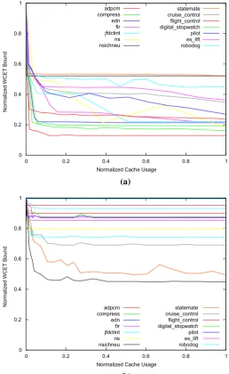
Figures1and2show the normalized WCET bounds for the benchmark tasks with varying cache partition sizes and cache types. Each line denotes the execution time for one benchmark. The y-axis depicts the normalized execution time with the value 1 representing the largest WCET bound (which typically corresponds to the smallest cache partition size i.e. zero). The x-axis depicts the normalized cache partition size with the value 1 representing the code-size/maximum memory usage of the task. Increasing the size of the cache partition beyond the code size/memory footprint does not improve the execution time any further. The graphs are best viewed online in colour. A perfect data (or instruction) cache means that all data (or instruction) accesses are served instantaneously. Even though this assumption is unrealistic, it removes possible noise and and allows us to fully concentrate on the effects of pre-emption and partitioning. We have also performed experiments withinstruction cache but without

data cacheand also withdata cache but without instruction cache. The results are

very similar to the evaluation shown for perfect caches, but less accentuated. We can see that variation in the execution times is stronger in the case of instruction cache compared to data cache. This behaviour is as expected since each instruction results in an instruction cache access, but not necessarily in a data cache access. Similarly, the variation in the execution times is amplified by the assumption of a perfect data/instruction cache. Note we do not assume any implementation cost for cache partitioning. Additional delays to implement cache partitioning only occur if no native support for partitioning is available.

0 0.2 0.4 0.6 0.8 1

0 0.2 0.4 0.6 0.8 1

Normalized WCET Bound

Normalized Cache Usage I4 I5 I6 I7 T5 T6

T7 T8 T9 T10 T11 T12

(a)

0 0.2 0.4 0.6 0.8 1

0 0.2 0.4 0.6 0.8 1

Normalized WCET Bound

Normalized Cache Usage I4 I5 I6 I7 T5 T6

T7 T8 T9 T10 T11 T12

(b)

Fig. 1 WCETs depending on the cache partition size (PapaBench, see Table1).aDirect mapped instruction cache, perfect data cache.bDirect mapped data cache, perfect instruction cache

5.1.1 Monotonicity

We observe from Figs.1 and2 that the execution time bounds are not necessarily monotonic with respect to the cache partition size.

0 0.2 0.4 0.6 0.8 1

0 0.2 0.4 0.6 0.8 1

Normalized WCET Bound

Normalized Cache Usage adpcm

compress edn fir jfdctint ns nsichneu

statemate cruise_control flight_control digital_stopwatch pilot es_lift robodog

(a)

0 0.2 0.4 0.6 0.8 1

0 0.2 0.4 0.6 0.8 1

Normalized WCET Bound

Normalized Cache Usage adpcm

compress edn fir jfdctint ns nsichneu

statemate cruise_control flight_control digital_stopwatch pilot es_lift robodog

(b)

Fig. 2 WCETs depending on the cache partition size (Mälardalen and SCADE Benchmarks, see Table3). adirect mapped instruction cache, perfect data cache,bdirect mapped data cache, perfect instruction cache

0x00030→0x00080→0x00030

0 0.2 0.4 0.6 0.8 1

0 0.2 0.4 0.6 0.8 1

Normalized WCET Bound

Normalized Cache Usage

Upper bound basic function Lower bound

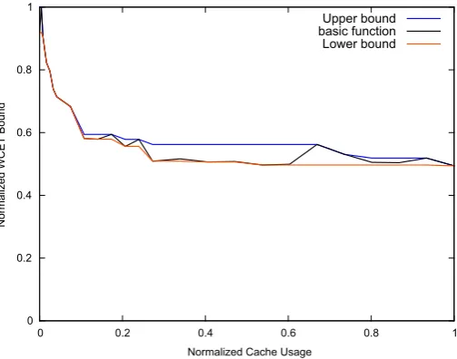
Fig. 3 Over-/underapproximations of the WCET function (statematebenchmark, direct mapped data cache, perfect instruction cache)

cache miss. Hence, for this trivial example, the performance with 5 cache sets is worse than that for 4 cache sets.

We note that the assumption of monotonic execution time bounds is both common and often not explicitly stated in work on cache partitioning for real-time systems (Bui et al. 2008; Busquets-Mataix and Wellings 1997; Kirk and Strosnider 1990; Mueller1995; Plazar et al.2009).

The impact of these effects is however limited, and so we can replace the actual execution time function with monotonic over/under-approximations without signif-icant loss of precision, as shown in Fig. 3. Here, the basic function (black line) is non-monotonic, while the upper bound (blue line) and the lower bound (red line) are monotonically non-increasing functions of cache partition size. We thus establish monotonicity of the WCET with respect to the cache partition size and can use this property in our approach to partitioning the cache. In Sect.8.5, we quantify the error introduced by this approximation.

5.2 Partition-size sensitivity (task group level)

0s 16.5s

WCET Bound

WCET

0 30

0 32 64 96 128 160 192 224 256

#Useful Cache Blocks

Partition Size

UCBs

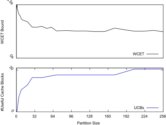
Fig. 4 WCET and number of UCBs depending on the cache partition size (statematebenchmark, direct mapped data cache, perfect instruction cache)

In case of a shared cache partition, two opposing factors influence the system’s performance: the execution time bounds and the pre-emption costs. Whereas the exe-cution time bounds typically increase when the size of the assigned cache partition is reduced, the pre-emption costs decrease. A smaller cache results in a higher number of intra-task conflicts and hence, in fewer cache hits without pre-emption. Figure4 depicts this behaviour. We note that a change in the maximum number of useful cache blocks always co-incides with a change in the execution time bound, whereas a change in the execution time bound does not necessarily imply a change in the maximum num-ber of useful cache blocks. Furthermore under the hardware restrictions assumed in this paper (set-based partitioned, LRU or direct-mapped caches), the impact of the execution time limits the impact of the pre-emption costs: The pre-emption costs can only increase, if the number of cached and re-used memory blocks increases, which means that the execution time decreases. The decrease in the execution time always dominates the increase in the pre-emption costs. When the number of potentially evicted memory blocks increases, then the execution time decreases at least by the time to reload these additional memory blocks times how often these memory blocks need to be reloaded. A large number of pre-emptions will then at most cancel out the decrease in the execution time, but never exceed it.

However, the dominance relation between the execution time bound and the pre-emption costs is not necessarily reflected in these schedulability analyses: The terms

sustainable for taskgroups, even under the assumption of monotonic execution times. This unsustainability of the schedulability tests means that the algorithms described in Sect.6would not retain their optimality if extended to the case where groups of tasks share partitions: False negatives are possible in the sense that no feasible shared cache partition is found although one may exist.

6 Optimal cache partitioning

In this section, we derive an optimal cache partitioning algorithm, which makes use of the monotonic upper bound execution time functions of cache partition size described in the previous section. We assume a direct-mapped cache of size S. A cache parti-tioningPis a tuple of non-negative integers describing for each taskτi, the sizepi of its allocated cache partition:

P =(p1,p2, . . . ,pn):N× · · · ×N

n

(32)

We assume that each task has a dedicated cache partition which is not shared with any other tasks (we return to this point in Sect.9). A cache partitioning is valid, if the total size of the cache partitions does not exceed the overall sizeSof the cache (i.e. if

i pi ≤ S).

6.1 Schedulability

We are interested in the schedulability of a taskset, as this is the main optimization criterion for hard real-time systems. We therefore say that a cache partitioning algo-rithm is optimal, iff it finds a cache partitioning whereby the tasks are schedulable, whenever such a partitioning exists. Note that this is different from minimizing the utilization of a taskset, since taskset utilization is only a rough indicator of system schedulability.

To compute an optimal cache partitioning, we use a branch-and-bound approach (see Algorithm 1) which is certain, under the assumption of monotonic execution time functions, to find a feasible cache partitioning if one exists. To this end, we exploit the sustainability of the schedulability test with respect to execution times and the monotonicity of the execution time function with respect to the cache partition size to prune the search space.

The algorithm is implemented using a recursive functioncheckPartition. This func-tion takes as its input the current task indexi, a partially defined partitioning P and the remaining cache sizes. The partitioning is defined up to indexi and the remain-ing cache sizesis given bySminus the sum of the sizes of the firsti partitions i.e.

s=S−i_j=1pi.

The initial input to the function is the first task index 1, an arbitrary partitioningP

basic schedulability tests without pre-emption costs (see Sect. 3) given by (2) and (16), as the cache partitioning prevents any cache-related pre-emption delays.

In the next step, the algorithm checks taskset schedulability under (a) the optimistic assumption that each not yet specified task partition is of sizes and (b) under the pessimistic assumption that each not yet specified task partition is given an equal share of the remaining cache size, i.e.,⌊s/(n−i+1)⌋. This enables effective pruning of the search in the case where (a) schedulability is disproved for any extensions to the current partial partitioning, and early exit in the case (b) schedulability is proven assuming that all further tasks are schedulable with a cache partition of equal size.

The last construct of the algorithm, the while loop, implements the branching. The partition size of cache partition pi is varied from 0 up to the remaining cache sizes and each possible partitioning is evaluated using a recursive function call. This is done using the functionnextStepwhich computes the next partition size for taskτi. Due to the monotonicity of the execution time functions with respect to cache partition size,

nextStepjumps directly to the next partition size where the execution time changes.

All intermediate partition sizes with the same execution time can be safely ignored. In the worst-case, up tonS different cache partitionings must be evaluated, wheren

6.2 Schedulability and minimal utilization

Algorithm 1 can be extended to find a schedulable cache partitioning with the minimum processor utilization (see Algorithm 2). Schedulability is usually the dominating cri-terion for hard real-time systems but a reduced processor utilization typically reduces the energy consumption and the response times and thus improves the overal perfor-mance of the system.

The global variableminUtilis initially set to 1.1 to indicate that no schedulable cache partitioning has been found yet. As soon as the algorithm encounters a schedulable partitioning, the utilization is computed and compared tominUtil(which is updated if necessary).

the weaker abort-condition of Algorithm 2, a significantly higher number of cache partitionings must be evaluated when a schedulable partitioning exists. When no such partitioning exists, both algorithm consider exactly the same number of partitionings. We evaluate the difference in the average processor utilization and analysis time for the two algorithms in Sect.7.3.

7 Case study

In this section, we evaluate the partitioning algorithms based on PapaBench (Nemer et al. 2006), the Mälardalen benchmark suite (Gustafsson et al.2010) and a set of SCADE4tasks (partially provided by SCADE, partially from our own SCADE mod-els). Besides the effectiveness of the cache partitioning algorithms, we are interested in (i) the precision of the simplified execution time model, (ii) the runtime performance of the algorithms, and (iii) the difference between the two partitioning algorithms with respect to the minimum utilization obtained.

For the case study, the target architecture is an ARM7 processor (with a 4 kB direct-mapped write-through cache, line size of 16 Bytes, 256 cache sets, block reload time 8µs, clock rate of 100 MHz). The execution time bounds were derived using the aiT Timing analyzer (Ferdinand and Heckmann2004). The values are derived from an example configuration of the ARM7 as used in previous work (see Altmeyer et al. 2011).

Papabench provides two different tasksets (fbwandautopilot) with deadlines and periods (except for the interrupts I4 to I7) (see Tables1and2). With the initial processor frequency of 100 MHz, both tasksets are schedulable both with and without cache partitioning. The other benchmarks only provide code and do not form a meaningful taskset. We therefore randomly selected tasks from (i) Tables1and2, and (ii) Table3 and4(together with execution times, the execution time variations, codes size and UCBs/ECBs).

The remaining task and taskset parameters used in our experiments were randomly generated as follows:

– The default taskset size was 10.

– Task utilizations were generated using the UUnifast (Bini and Buttazzo2005) algorithm.

– Task periods were set based on the utilization and execution times:Ci =Ui ·Ti. – Task deadlines were implicit,5i.e.,Di =Ti.

– For fixed priority scheduling, priorities were assigned in Rate Monotonic priority order.

The tasks are indexed and processed by the partioning algorithms in decreasing priority order.

In each experiment the taskset utilization not including pre-emption cost was varied from 0.025 to 0.975 in steps of 0.025. For each utilization value, 1000 tasksets were

4 _{Esterel SCADEhttp://www.esterel-technologies.com/.}

5 _{Evaluation for constrained deadlines, i.e.,D}

i ∈ [2Ci;TI]gave broadly similar results although fewer

Table 1 Execution times and number of UCBs and ECBs for the PapaBench benchmarks

Description UCBs ECBs WCET1 WCET2 Period

I4 Interrupt-modem 2 10 303µs 520µs –

I5 Interrupt-spi-1 1 10 251µs 447µs –

I6 Interrupt-spi-2 1 4 151µs 228µs –

I7 Interrupt-gps 3 26 283µs 493µs –

T5 Altitude-control 20 66 1478µs 1660µs 250 ms

T6 Climb-control 1 210 5429µs 6241µs 250 ms

T7 Link-fbw-send 1 10 233µs 471µs 250 ms

T8 Navigation 1 256 44, 42 ms 54, 35 ms 50 ms

T9 Radio-control 0 256 15, 6 ms 21, 1 ms 50 ms

T10 Receive-gps-data 22 194 5987µs 6659µs 25 ms

T11 Reporting 2 256 12, 22 ms 5 ms 100 ms

T12 Stabilization 11 194 5681µs 6654µs 50 ms

Data cache with perfect instruction cache (W C E T1) and without data cache (W C E T2)

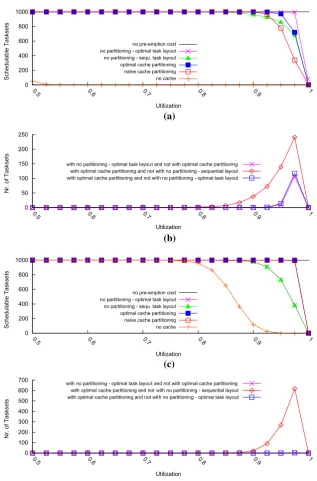
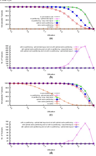
generated and the schedulability of those tasksets was determined using the cache partitioning algorithms or pre-emption cost aware analysis with either sequential or optimal task layout (Lunniss et al.2012). We thus compared the results for cache partitioning against those for (i) no partitioning with a sequential task layout, (ii) no partitioning with an optimized task layout, (iii) analysis ignoring pre-emption costs, but assuming that all the tasks shared the cache; (iv) naive cache partitioning with all tasks allocated the same size partitionS/n; (v) no cache. The sequential task layout reflects the basic un-optimized cache mapping, i.e., where the code for each task is placed consecutively in memory. In case of unconstrained cache usage, we used the combined multiset approaches for fixed-priority (14) and for EDF scheduling (31) to compute the schedulability of the tasksets.

For fixed priority scheduling, we were able to compute the schedulability of all tasksets (42,000 tasksets per case study) in less than 10 min on a 2.6-GHz Quadcore processor—despite the exponential worst-case behaviour of the cache partitioning algorithm (Algorithm 1). For EDF scheduling, the computation for the same config-urations took about 60 min. This shows a more than acceptable analysis time for the partitioning algorithm, with a strong dependency on the runtime of the schedulability test that it uses.

7.1 PapaBench

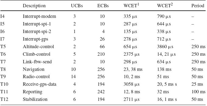
Table 2 Execution times and number of UCBs and ECBs for the PapaBench benchmarks

Description UCBs ECBs WCET1 WCET2 Period

I4 Interrupt-modem 3 10 335µs 790µs –

I5 Interrupt-spi-1 2 10 287µs 644µs –

I6 Interrupt-spi-2 1 4 135µs 338µs –

I7 Interrupt-gps 3 26 278µs 712µs –

T5 Altitude-control 2 66 654µs 3860µs 250 ms

T6 Climb-control 5 210 2375µs 14, 21µs 250 ms

T7 Link-fbw-send 2 10 298µs 634µs 250 ms

T8 Navigation 10 256 23, 38 ms 138 ms 50 ms

T9 Radio-control 14 256 10, 2 ms 51 ms 50 ms

T10 Receive-gps-data 4 194 3058µs 20, 5 ms s 25 ms

T11 Reporting 6 242 12, 8 ms 32 ms 100 ms

T12 Stabilization 6 194 2711µs 16, 1 ms s 50 ms

Data cache with perfect instruction cache (W C E T1) and without instruction cache (W C E T2)

caches (Figs.5b and6b), optimal partitioning has similar performance to sequential task layout with no partitioning, while optimal task layout with no partitioning results in improved performance. Optimal cache partitioning was only able to improve per-formance over sequential task layout with no partitioning in a few cases. In the case of data caches(Figs.5d and6d), optimal partitioning outperforms optimal task layout with no partitioning. The variation of the execution times in this case is rather low, while the number of UCBs is comparably high. We thus note that the two approaches

areincomparable. Almost no tasksets were schedulable with no cache, except for the

case of data cache with perfect instruction cache as the impact of the data cache alone is limited.

With respect to the scheduling policy, i.e. fixed priority vs. EDF, there was no sig-nificant difference in the relative performance of the various approaches. As expected, the schedulability tests for EDF deem consistently more tasksets schedulable (for all approaches) than those for fixed priority scheduling.

7.2 Mälardalen and SCADE benchmarks

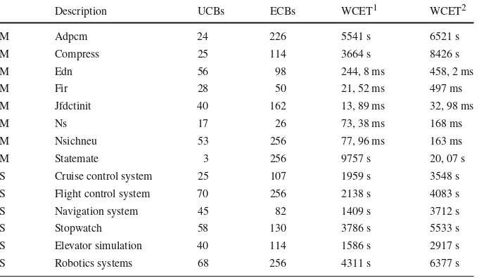
Table 3 Mälardalen benchmark suite (M) and SCADE benchmarks (S)

Description UCBs ECBs WCET1 WCET2

M Adpcm 24 226 5541 s 6521 s

M Compress 25 114 3664 s 8426 s

M Edn 56 98 244, 8 ms 458, 2 ms

M Fir 28 50 21, 52 ms 497 ms

M Jfdctinit 40 162 13, 89 ms 32, 98 ms

M Ns 17 26 73, 38 ms 168 ms

M Nsichneu 53 256 77, 96 ms 163 ms

M Statemate 3 256 9757 s 20, 07 s

S Cruise control system 25 107 1959 s 3548 s

S Flight control system 70 256 2138 s 4083 s

S Navigation system 45 82 1409 s 3712 s

S Stopwatch 58 130 3786 s 5533 s

S Elevator simulation 40 114 1586 s 2917 s

S Robotics systems 68 256 4311 s 6377 s

Data cache with perfect instruction cache (W C E T1) and without data cache (W C E T2)

Table 4 Mälardalen benchmark suite (M) and SCADE benchmarks (S)

Description UCBs ECBs WCET1 WCET2

M Adpcm 7 242 5856 s 43, 17 s

M Compress 6 242 9740 s 25, 26 s

M Edn 5 98 518, 9 ms 1422 s

M Fir 5 50 42, 65 ms 121 ms

M Jfdctinit 8 242 23, 2 ms 73, 63 ms

M Ns 3 26 133, 7 ms 466, 9 ms

M Nsichneu 8 242 66, 74 ms 178, 3 ms

M Statemate 30 242 8143 s 22, 45 s

S Cruise control system 15 98 1, 77 s 6207 s

S Flight control system 12 242 3, 24 s 11, 02 s

S Navigation system 3 82 2, 96 s 7566 s

S Stopwatch 9 130 4417 s 25, 03s

S Elevator simulation 4 114 1863 s 5432 s

S Robotics systems 5 242 3427 s 22, 45 s

Data cache with perfect instruction cache (W C E T1) and without instruction cache (W C E T2)

7.3 Utilization versus analysis time

0 200 400 600 800 1000

0.5 0.6 0.7 0.8 0.9 1

Schedulable T

asksets

Utilization

no pre-emption cost no partitioning - optimal task layout no partitioning - sequ. task layout optimal cache partitioning naive cache partitioning no cache

(a₎

(b)

(c)

(d) 0 20 40 60 80 100 120 140 160 180

0.5 0.6 0.7 0.8 0.9 1

Nr. of T

asksets

Utilization

with no partitioning - optimal task layout and not with optimal cache partitioning with optimal cache partitioning and not with no partitioning - sequential layout with optimal cache partitioning and not with no partitioning - optimal task layout

0 200 400 600 800 1000

0.5 0.6 0.7 0.8 0.9 1

Schedulable T

a

sksets

Utilization

no pre-emption cost no partitioning - optimal task layout no partitioning - sequ. task layout optimal cache partitioning naive cache partitioning no cache 0 50 100 150 200 250 300 350

0.5 0.6 0.7 0.8 0.9 1

Nr. of T

a

sksets

Utilization

with no partitioning - optimal task layout and not with optimal cache partitioning with optimal cache partitioning and not with no partitioning - sequential layout with optimal cache partitioning and not with no partitioning - optimal task layout

0 200 400 600 800 1000

0.5 0.6 0.7 0.8 0.9 1

Schedulable T asksets Utilization (a) (b) (c) (d)

no pre-emption cost no partitioning - optimal task layout no partitioning - sequ. task layout optimal cache partitioning naive cache partitioning no cache 0 50 100 150 200 250

0.5 0.6 0.7 0.8 0.9 1

Nr. of T

a

sksets

Utilization

with no partitioning - optimal task layou t and not with optimal cache partitioning with optimal cache partitioning and not with no partitioning - sequential layout with optimal cache partitioning and not with no partitioning - optimal task layout

0 200 400 600 800 1000

0.5 0.6 0.7 0.8 0.9 1

Schedulable T

asksets

Utilization

no pre-emption cost no partitioning - optimal task layout no partitioning - sequ. task layout optimal cache partitioning naive cache partitioning no cache 0 100 200 300 400 500 600 700

0.5 0.6 0.7 0.8 0.9 1

Nr. of T

a

sksets

Utilization

with no partitioning - optimal task layou t and not with optimal cache partitioning with optimal cache partitioning and not with no partitioning - sequential layout with optimal cache partitioning and not with no partitioning - optimal task layout

0 200 400 600 800 1000

0.5 0.6 0.7 0.8 0.9 1

Schedulable T

a

sksets

Utilization

(a)

(b)

(c)

(d) no pre-emption cost no partitioning - optimal task layout no partitioning - sequ. task layout optimal cache partitioning naive cache partitioning no cache 0 50 100 150 200 250 300 350 400 450 500

0.5 0.6 0.7 0.8 0.9 1

Nr. of T

a

sksets

Utilization

with no partitioning - optimal task layou t and not with optimal cache partitioning with optimal cache partitioning and not with no partitioning - sequential layout with optimal cache partitioning and not wit h no partitioning - optimal task layout

0 200 400 600 800 1000

0.5 0.6 0.7 0.8 0.9 1

Schedulable T

a

sksets

Utilization

no pre-emption cost no partitioning - optimal task layout no partitioning - sequ. task layout optimal cache partitioning naive cache partitioning no cache 0 20 40 60 80 100 120 140 160

0.5 0.6 0.7 0.8 0.9 1

Nr. of T

a

sksets

Utilization

with no partitioning - optimal task layout and not with optimal cache partitioning with optimal cache partitioning and not with no partitioning - sequential layout with optimal cache partitioning and not with no partitioning - optimal task layout

0 200 400 600 800 1000

0.5 0.6 0.7 0.8 0.9 1

Schedulable T

a

sksets

Utilization (a₎

(b)

(c)

(d₎ no pre-emption cost no partitioning - optimal task layout no partitioning - sequ. task layout optimal cache partitioning naive cache partitioning no cache 0 100 200 300 400 500 600 700 800

0.5 0.6 0.7 0.8 0.9 1

Nr. of T

a

sksets

Utilization

with no partitioning - optimal task layout and not with optimal cache partitioning with optimal cache partitioning and not with no partitioning - sequential layout with optimal cache partitioning and not with no partitioning - optimal task layout

0 200 400 600 800 1000

0.5 0.6 0.7 0.8 0.9 1

Schedulable T

asksets

Utilization

no pre-emption cost no partitioning - optimal task layout no partitioning - sequ. task layout optimal cache partitioning naive cache partitioning no cache 0 50 100 150 200 250

0.5 0.6 0.7 0.8 0.9 1

Nr. of T

a

sksets

Utilization

with no partitioning - optimal task layout and not with optimal cache partitioning with optimal cache partitioning and not with no partitioning - sequential layout with optimal cache partitioning and not with no partitioning - optimal task layout

0 0.5 1 1.5 2 2.5 3 3.5

0 0.1 0.2 0.3 0.4 0.5 0.6 0.7 0.8 0.9 1

increased utilization (%)

nominal utilization FP with optimized utilization

FP without optimized utilization

0 1 2 3 4 5 6 7 8

0 0.2 0.4 0.6 0.8 1

analysis time (seconds)

nominal utilization (a)

(b) FP with optimized utilization FP without optimized utilization

Fig. 9 Evaluation of the average utilization PapaBench benchmarks (fixed priority scheduling, instruction cache with perfect data cache).aAverage utilization of schedulable tasksets per nominal utilization,btotal analysis time for 1000 tasksets

with minimum utilization. To this end, we compare the results and analysis times of both algorithms presented in Sect.6, i.e. with and without optimizing minimum processor utilization as a secondary concern.

The results of this comparison are shown in Figs.9 and10for the PapaBench benchmark suite and in Figs.11and12for the Mälardalen benchmark suite. Sub-figures (a) show the average percentage increase in processor utilization (i.e. with the execution time overhead due to cache partitioning) of schedulable tasksets with respect to the nominal utilization (i.e. without execution time overhead due to cache partitioning). Subfigures (b) show the analysis time for all 1000 tasksets generated per utilization level. The blue line representes the optimal cache paritioning algorithm without optimized utilization (Algorithm 1) and the pink line with optimized utiliza-tion (Algorithm 2). We have omitted the results for data cache with perfect instrucutiliza-tion cache as they resemble the results for instruction cache with perfect data cache, with a less significant difference.

0 0.5 1 1.5 2 2.5 3 3.5

0 0.2 0.4 0.6 0.8 1

increased utilization (%)

nominal utilization EDF with optimized utilization

EDF without optimized utilization

(a)

0 50 100 150 200 250

0 0.2 0.4 0.6 0.8 1

analysis time (seconds)

nominal utilization EDF with optimized utilization EDF without optimized utilization

(b)

Fig. 10 Evaluation of the average utilization PapaBench benchmarks (EDF scheduling, instruction cache with perfect data cache).aAverage utilization of schedulable tasksets per nominal utilization,btotal analysis time for 1000 tasksets

In contrast to the processor utilization, the difference in the total analysis time is noticable in all cases, especially if the nominal processor utilization is above 0.8. This indicates that the algorithm to optimize the processor utilization requires a significant amount of time to either find an improved cache partitioning or to show the optimality of the current candidate. We conclude that a small but nevertheless useful improvement in utilization can be obtained using Algorithm 2; however, that this comes at a cost in terms of increased runtime of the analysis.

We note that the average increase in utilization which occurs using Algorithm 1 is similar for both fixed priority and EDF scheduling with the only difference beeing that the increase drops at a lower nominal utilization for fixed-priority scheduling (0.8) than for EDF scheduling (0.85). This is because EDF has a schedulable utilization bound of 1 (much higher than that for fixed priority scheduling), thus a careful tuning of the partition size to achieve a schedulable partitioning is only required at higher nominal utilizations. The reduced difference in the nominal utilization also coincides in both cases (fixed-priority and EDF) with an increase in the analysis time of Algorithm 1.

Note, as both algorithms behave similar in case no schedulable cache partition-ing exists, the differences in the analysis time are only due to the optimization of

0 1 2 3 4 5 6 7

0 0.2 0.4 0.6 0.8 1

increased utilization (%)

nominal utilization FP with optimized utilization

FP without optimized utilization

(a)

(b)

0 5 10 15 20 25 30 35 40

0 0.2 0.4 0.6 0.8 1

analysis time (seconds)

nominal utilization FP with optimized utilization FP without optimized utilization

Fig. 11 Evaluation of the average utilization of Mälardalen benchmarks (fixed priority scheduling, instruc-tion cache with perfect data cache).aAverage utilization of schedulable tasksets per nominal utilization,b total analysis time for 1000 tasksets

8 Synthetic tasksets

We also evaluated the effectiveness of cache partitioning on a large number of syn-thetic tasksets with varying cache configurations and varying task parameters. Our aim here was to identify those parameters that have a significant influence on the rela-tive effecrela-tiveness of cache partitioning versus a non-partitioned cache. The evaluation using randomly generated tasksets enables us to fully control all relevant parameters, which is not possible using the benchmark tasks directly.

The task parameters used in our experiments were randomly generated as follows:

– The default taskset size was 10.

– Task utilizations were generated using the UUnifast (Bini and Buttazzo2005) algo-rithm.

– Task periods were generated according to a log-uniform distribution with a factor of 1000 difference between the minimum and maximum possible task period and a minimum period of 5 ms. This represents a spread of task periods from 5 ms to 5 s, thus providing reasonable correspondence with real systems.

– Task execution times were set based on the utilization and period selected:Ci =

Ui·Ti.