Modeling soil organic carbon dynamics in temperate forests with Yasso07

https://doi.org/10.5194/bg-16-1955-2019 © Author(s) 2019. This work is distributed under the Creative Commons Attribution 4.0 License.

Modeling soil organic carbon dynamics in temperate

forests with Yasso07

Zhun Mao1,8, Delphine Derrien1, Markus Didion2, Jari Liski3,9, Thomas Eglin4, Manuel Nicolas5, Mathieu Jonard6, and Laurent Saint-André1,7

1_{INRA, UR BEF – Biogéochimie des Ecosystèmes Forestiers, 54280 Champenoux, France}

2_{Swiss Federal Institute for Forest, Snow and Landscape Research WSL, 8903 Birmensdorf, Switzerland} 3_{Finnish Environment Institute, Ecosystem Change Unit, Natural Environment Centre, Mechelininkatu 34a,}

P.O. Box 140, 00251 Helsinki, Finland

4_{ADEME – DPED – Service Agriculture et Forêts, 49004 Angers, France}

5_{Office National des Forêts, Direction Forêts et Risques Naturels, Département Recherche-Développement-Innovation,}

Boulevard de Constance, 77300 Fontainebleau, France

6_{Earth and Life Institute, Université Catholique de Louvain, Croix du Sud 2, L7.05.09,}

1348 Louvain-la-Neuve, Belgium

7_{CIRAD, UMR ECO&Sols, Place Viala, 34398 Montpellier Cedex 5, France} 8_{Amap, INRA, CNRS, IRD, CIRAD, University Montpellier, Montpellier, France} 9_{Finnish Meteorological Institute, P.O. Box 503, 00101 Helsinki, Finland}

Correspondence:Zhun Mao (maozhun04@126.com) Received: 30 April 2018 – Discussion started: 18 June 2018

Revised: 27 January 2019 – Accepted: 1 April 2019 – Published: 13 May 2019

Abstract.In a context of global changes, modeling and pre-dicting the dynamics of soil carbon stocks (CSs) in forest ecosystems are vital but challenging. Yasso07 is considered to be one of the most promising models for such a purpose. We examine the accuracy of its prediction of soil carbon dy-namics over the whole French metropolitan territory at a de-cennial timescale.

We used data from 101 sites in the RENECOFOR net-work, which encompasses most of the French temperate forests. These data include (i) the quantity of above-ground litterfall from 1994 to 2008, measured yearly, and (ii) the soil CSs measured twice at an interval of approximately 15 years (once in the early 1990s and around 2010). We used Yasso07 to simulate the annual changes in carbon stocks (ACCs; in tC ha−1yr−1) for each site and then compared the estimates with actual recorded data. We carried out meta-analyses to reveal the variability in litter biochemistry in different tree organs for conifers and broadleaves. We also performed sen-sitivity analyses to explore Yasso07’s sensen-sitivity to annual litter inputs and model initialization settings.

At the national level, the simulated ACCs (+0.00± 0.07 tC ha−1yr−1, mean±SE) were of the same order of magnitude as the observed ones (+0.34±0.06 tC ha−1_yr−1_).

However, the correlation between predicted and measured ACCs remained weak (R2<0.1). There was significant over-estimation for broadleaved stands and underover-estimation for coniferous sites. Sensitivity analyses showed that the final es-timated CS was strongly affected by settings in the model ini-tialization, including litter and soil carbon quantity and qual-ity and also by simulation length. Carbon qualqual-ity set with the partial steady-state assumption gave a better fit than the model with the complete steady-state assumption.

1 Introduction

The current global carbon stock (CS) in soils, including for-est litter and peatlands, is 1500 to 2400 GtC and thus greatly exceeds stocks in vegetation, found mainly in forests (350 to 550 GtC) and in the atmosphere (829 GtC in 2011; IPCC, 2014). Soils share a common interface with all the other spheres and play a key role in driving the global carbon cy-cle. Soil CS dynamics are directly related to the greenhouse gas emissions (notably carbon dioxide; CO2) that are

lead-ing to the global warmlead-ing effect (IPCC, 2014). An accurate estimation of soil CS dynamics would allow us to better un-derstand the turnover rate and fate of soil carbon flux at both local and global geographical scales. In the context of global changes, accurate estimation is essential in evaluating the cli-mate change mitigation potential of forests and supporting environmental policy decisions.

Significant challenges exist when attempting to accurately estimate changes in soil CSs. Current soil monitoring net-works are generally not able to detect changes on timescales of less than 10 years (Saby et al., 2008). To obtain estimates for changes in soil CSs at shorter intervals, as is, for example, required for annual reporting to the United Nations Frame-work Convention on Climate Change and the Kyoto Protocol, using models is encouraged (IPCC, 2011). Numerous mod-els have been elaborated to evaluate soil carbon dynamics (Manzoni and Porporato, 2009). The vast majority of terres-trial soil carbon models developed at the global or the plot scale (e.g., CENTURY in Parton et al., 1987; RothC in Cole-man and Jenkinson, 1996; and ORCHIDEE in Krinner et al., 2005) assume that decomposition is the first-order decaying process, which accounts for the size of soil carbon pools. However, the assumption has been criticized, and it has been argued that a priming effect and the associated carbon pool interactions should also be considered in model algorithms (Wutzler and Reichstein, 2013). The dynamics of carbon pools depend on the quantity and quality of litter inputs and on temperature, soil moisture and other soil parameters, e.g., texture, structure, chemical richness, pH, etc. (Todd-Brown et al., 2012). Incorporating explicit mechanisms such as mi-crobial activities or carbon protection by the soil matrix into soil carbon models has repeatedly been suggested in recent years (Schmidt et al., 2011; Lehmann and Kleber, 2015). However, for forest ecosystems, refined mechanistic input data often remain limited. Accordingly, the typical time step for litter input demanded by most forest soil carbon mod-els is yearly, rather than monthly (but see RothC, Coleman and Jenkinson, 1996) or daily (but see Romul in Chertov et al., 2001; Didion et al., 2016). At this yearly timescale, it is common to consider microbial communities and processes to be relatively stable factors (Todd-Brown et al., 2012); in this case, the assumption that carbon dynamics are governed by first-order decay may therefore be reasonable.

This is the choice made by the group who built the Yasso (Liski et al., 2005) and Yasso07 (Tuomi et al., 2009, 2011a,

b) models. Yasso07 is an improved version of Yasso with more refined carbon pooling and abundant data for calibra-tion. The model developers’ intention was to make their models suitable for general forestry applications by taking into account the limited availability of forest soil and litter data (Liski et al., 2005). Yasso07 explicitly defines several pools of chemical compounds in litter carbon (Tuomi et al., 2011b) and possesses well defined, biologically meaningful and measurable parameters. Thanks to these qualities, Yasso or Yasso07 has been applied in more than 150 case stud-ies (https://en.ilmatieteenlaitos.fi/yasso-publications, last ac-cess: 21 April 2019) in forest ecosystems in the Northern Hemisphere, with generally high satisfaction levels when compared with measured carbon values (e.g., Karhu et al., 2011; Rantakari et al., 2012; Ortiz et al., 2013; Didion et al., 2014; Lu et al., 2015; Wu et al., 2015). Yet so far most of these applications have been limited to local case studies, especially in cold forests with limited tree species diversity (e.g., boreal or montane forests). Rarely have previous stud-ies validated Yasso07 based on data (i) from long-term ob-servations (here defined as >10 years), (ii) from temperate forests with a much higher diversity of tree species or (iii) on changes in CSs (in tC ha−1yr−1). This is partially due to the lack of extensive long-term soil carbon monitoring in forest ecosystems, which differs in climatic and soil conditions and species and stretches over large territorial scales. Neverthe-less, Yasso07 is considered to be one of the potentially appro-priate models for evaluating national and continental inven-tories of the forest carbon balance in Europe (Hernández et al., 2017). It is therefore of considerable interest to assess the ability of Yasso07 to reflect the carbon balance in different European forest ecosystems at large spatio-temporal scales. Moreover, as a carbon-pool-based model, Yasso07 shares certain principles with other prevailing soil carbon models in the same genre (e.g., RothC, CENTURY, etc.). Applying Yasso07 as an example model in this case study may also allow us to improve future carbon modeling for temperate forests in general.

min-imize this source of uncertainty and focus on the inherent model structure.

We hope to contribute to the further development of soil carbon modeling by (i) testing and characterizing the ability of Yasso07 to model soil CS dynamics for temperate forests, (ii) identifying limitations and providing suggestions for a better adaptation of the model for C dynamics in both decid-uous and evergreen temperate forests, and (iii) discussing the perspectives based on the current state of the art in soil car-bon modeling. Associated with the above aims, our null hy-potheses are as follows: (i) Yasso07 predicts accurate and un-biased CS changes at the national scale, and (ii) the model’s fit residuals (predicted data minus observed data) have null relationships with site characteristics (e.g., location, climate, forest type, soil type and initial CS).

2 Materials and methods 2.1 The Yasso07 model

The Yasso07 dynamic soil carbon model is based on the gen-eral assumption that the soil CS is driven by the decomposi-tion of different litter types, which may differ in quantity and quality and by climatic conditions. Litter carbon quality is represented by four chemical compound groups with differ-ent decomposition rates (Tuomi et al., 2009). Soil organic carbon is divided into these four relatively labile carbon pools and one recalcitrant pool called “humus” (H) (Fig. S1 in the Supplement). The five pools differ in specific mass loss rates and mass flows. As in many other pool-based models, the H pool is considered to be the oldest and most stable car-bon pool, although recent studies have thrown doubt on its stability and even its physical existence (see Lehmann and Kleber, 2015). Some mass flows correspond to CO2release

(microbial respiration). The mean residence time of carbon in these pools varies, lasting several months (i.e., water soluble compounds – W), a few years (i.e., acid-hydrolyzable com-pounds – A; non-polar solvent, ethanol or dichloromethane compounds – E), several decades (i.e., soluble and non-hydrolyzable compounds – N) or even several centuries (i.e., H).

Mathematically, the kernel equation of Yasso07 can be written as follows:

˙

X(t )=ApK(c)X(t ) I (t ), (1a)

where symbols in bold capital letters denote either vectors or matrices, while those in small letters in parentheses denote scalars,X(t )is the vector describing the masses of the five carbon pools (A, W, E, N and H) at timet,X(t )˙ is the vector describing carbon mass changes in soil at timet,Ap is the

mass flow matrix describing carbon allocation among pools, K(c)is the decomposition matrix describing the decomposi-tion rates as a funcdecomposi-tion of climatic condidecomposi-tions (c), and I (t ) is litter input to the soil and is equal to 0 for the last pool,

since “H” does not exist in litter form (Eq. 1a) and can be expressed in a more detailed form. This form is

   

∂xA/∂t

∂xW/∂t

∂xE/∂t

∂xN/∂t

∂xH/∂t    

=    

−1 pW→A pE→A pN→A 0

pA→W −1 pE→W pN→W 0

pA→E pW→E −1 pN→E 0

pA→N pW→N pE→N −1 0

pA→H pW→H pE→H pN→H −1    

     

kA 0 0 0 0

0 kW 0 0 0

0 0 kE 0 0

0 0 0 kN 0

0 0 0 0 kH

     

     

xA

xW

xE

xN

xH

     

+      

IA

IW

IE

IN

0      

, (1b)

wherepF→T is the relative mass flow parameter between

two pools (from F to T; F and T can be any two pools among A, W, E, N and H) in the soil (dimensionless, pF→T ∈[0, 1]).

Temperature and precipitation are assumed not to affect mass flowpbut do influence mass loss rateki (i=A, W, E,

N or H) according to the following:

ki(c)=αiexp

β1T+β2T2

1−exp(γ Pa)

, (2)

whereαiis the mass loss rate parameter of the chemical pool

i; andβ1,β2andγare parameters related to temperature (T;

in◦C) and precipitation (Pa; in mm).

To take into account the effect of litter size on the litter decomposition rate,ki was multiplied by a litter size factor

(hs), which makes it possible to distinguish between different

types of litter (e.g., foliage, coarse woody debris, stems, etc.), differing in diameter (d; in mm):

hs(d)=min

n

1+ϕ1d+ϕ2d2

r

,1o, (3)

whereϕ1,ϕ1andrare parameters related to litter size.

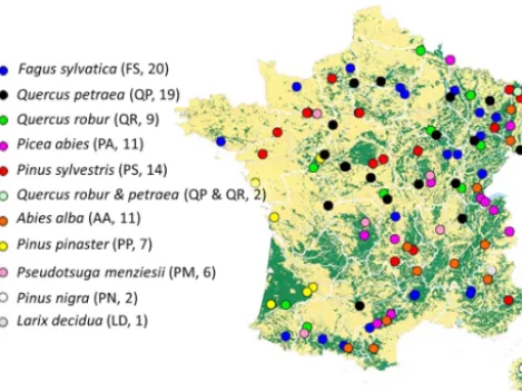
Figure 1.Geographical distribution of the sites in the RENECO-FOR network used to test Yasso07 performance (see also Jonard et al., 2017). Forested areas are represented in green. Each circle rep-resents one site; the color reprep-resents the dominant tree species on the plot. The species abbreviation and number of sites per species

are indicated in parentheses. One site (Picea abies39b) was not

used due to data incompletion.

stochastic effect. In this study, we adapted the Tuomi (2011) set to the RENECOFOR dataset.

2.2 RENECOFOR network

The RENECOFOR network is part of the Level II network of the International Co-operative Programme on Assessment and Monitoring of Air Pollution Effects on Forests (ICP Forests). The 101 sites (Fig. 1) considered in this study cover the most common types of forest ecosystems in France, in-cluding evenly aged forests in plains, pine plantations and unevenly aged mountain forests. They also host most of the tree species in France and central Europe, includingQuercus robur,Quercus petraea,Pseudotsuga Menziesii,Picea abies, Fagus sylvatica,Pinus pinaster,Pinus sylvestris andAbies alba. At each forest site, annual woody and non-woody litter quantities are either directly measured or estimated based on existing dendrometric data.

2.2.1 Soil carbon and soil physical and chemical properties

At each site, soil CSs were measured twice at an interval of approximately 15 years (1993–1995 for the first assessment and 2007–2012 for the second one). At each site and for each assessment, soils were sampled to a depth of 0.4 m at five points selected in each of five subplots, and the samples were divided into different layers (0–0.1, 0.1–0.2 and 0.2–0.4 m), including both organic and mineral soil layers. The tempo-ral changes in soil CSs to a depth of 0.4 m were analyzed by Jonard et al. (2017). Composite samples were produced for

each layer and subplot then analyzed for mass, bulk density, soil organic carbon, and physical and chemical properties, in-cluding texture (proportion of clay, silt and sand; in %); pH value; total nitrogen stock (in t ha−1), the carbon : nitrogen ratio (dimensionless); total phosphorus stock (in t ha−1); and stocks of exchangeable aluminum (Al), calcium (Ca), potas-sium (K) and magnepotas-sium (Mg; in kmol ha−1). We used the soil physical and chemical property data measured during the first assessment (1993–1995) for residual analyses (see Sect. 2.7)

Regarding the CSs from 0.4–1.0 m in depth, only data from the first assessment (1993–1995) were available. Soil samples were obtained from only one soil profile per site at two mineral layers (0.4–0.8 and 0.8–1.0 m). Bulk density and carbon concentrations measured at these layers were used to estimate soil CSs to a depth of 1.0 m. Table 2 summarizes the data source for each of the 101 sites in the RENECOFOR network (http://www.onf.fr/renecofor/sommaire/renecofor/ reseau/20090119-130815-828957/@@index.html, last ac-cess: 21 April 2019). More detailed information about each site and the soil sampling procedure is available in Supple-ment I (Table S1) and Jonard et al. (2017).

2.2.2 Climate data

The climate data required by Yasso07 include annual mean precipitation (mm) and annual maximum, mean and mini-mum temperatures (◦C). These measured data were obtained from the national Météo-France meteorological stations (http://www.meteofrance.com, last access: 21 April 2019) nearest to each RENECOFOR site.

2.3 Litter quantity

Litter input (in tC ha−1yr−1) comes from several sources (see Table 2). We assumed a 0.5 conversion factor between biomass (dry matter) and carbon (Thomas and Martin, 2012). Above-ground litter input from living trees includes leaves for broadleaves and needles for conifers, small branches, fruits and miscellaneous items (e.g., flowers, buds, etc.). Above-ground litterfall mass was measured annually be-tween 1994 and 2008. For sites where litter quantity data from 1992–1993 and 2009–2012 were lacking, we used the mean litter quantity of all the other years at the same site. The observed branch size in this above-ground category was less than 2 cm (fine branches). Branches and stems bigger than 2 cm due to natural mortality were rare (since they can be salvaged) and were therefore not included in our calcula-tions.

and six sites had 10–11 missing years. We assumed that the residues due to harvesting or storms would be coarse branches (> 4 cm in diameter, confirmed with the ONF) based on above-ground tree characteristics. The quantities were es-timated on the basis of repeated stand inventory data and species-specific height–girth relationships and biomass. Lit-ter input from stems was set to 0, since in most cases, stem wood was removed from the site after storm damage. Litter input from coarse woody roots was considered to be equal to total root biomass, which was estimated through meta-analysis-based allometric equations proposed by Cairns et al. (1997). More detailed information about forest invento-ries and storm events occurring at each site is available in Supplement I (Table S1).

Litter input from fine roots (here defined as roots of ≤ 5 mm in diameter), especially the finest ones with a diameter ≤2 mm, can significantly contribute to carbon sequestration in soils (Brunner et al., 2013; Kögel-Knabner et al., 2002; Berg and McClaugherty, 2008). Fine root litter was assumed to be proportional to that of foliage, which was measured in the RENECOFOR sites (see the following paragraph). Jonard et al. (2017) suggested using the generic equation published by Raich and Nadelhoffer (1989) and, simultane-ously, adopted the hypothesis that fine-root litter production represents about one-third of the carbon allocated to roots (Raich and Nadelhoffer, 1989):

Ifine root=0.333× 1.92×(100×Ifoliage)+130

×0.01, (4) whereIfine rootandIfoliageare the litter input of fine roots and

foliage, respectively (in tC ha−1yr−1).

The relationship between fine-root and foliage litter inputs can be highly variable depending on tree species, stand char-acteristics and climate, and the generic equation may not re-liably represent such variability. To counter this, we carried out a sensitivity analysis to investigate the response of the model fit to the choice of fine-root-to-foliage ratio varying from 0.1 to 4.0 (see Sects. 2.6 and 3.2). Yet, when applying the equation of Raich and Nadelhoffer (1989; Eq. 4) over all the RENECOFOR sites, we found that fine-root-to-foliage ratios had a median of 1.0 and a mean of 1.0–1.1 for both coniferous and broadleaved sites (Fig. S2). Hence, we chose to use the 1.0 ratio over all the RENECOFOR sites to present the outcomes of the model fit and residual analyses from the simulations (see Sect. 3.3). This facilitated our evaluation of site factors (e.g., dominant tree functional type, climatic and soil features) without adding a source of variability in-troduced by fine-root-to-foliage ratio.

2.4 Litter carbon quality

In the RENECOFOR network, there are no measured data for litter carbon quality, defined as the relative amount of lit-ter carbon belonging to four different carbon pools (A, W, E and N). Therefore, we carried out a meta-analysis of the data collected in the literature where authors used chemical

fractioning procedures or near-infrared spectroscopy (NIRS) techniques to measure litter carbon quality. The data were restricted to non-tropical areas. Chemical data on litter com-posed of coarse tree organs (e.g., stems, coarse branches) are relatively scarce, so we used the tree stem wood data com-piled in Pettersen (1984), Rowell et al. (2005) and Row-ell (2012). These three studies cover a wide range of tem-perate tree species from North America, Japan and Russia. Data on foliage and root litter carbon quality were taken either from networks such as CIDET (Trofymow, 1998) and LIDET (http://andrewsforest.oregonstate.edu/research/ intersite/lidet.htm, last access: 21 April 2019) or from inde-pendent studies in the Northern Hemisphere. The database we used for our meta-analysis is available in Supplement II. The root diameter or branching order can play a significant role in modifying the composition of soil chemical com-pounds (Fahay et al., 1988; Tingey et al., 2003; Guo et al., 2004). All the measurements included in our meta-analysis on roots refer to fine roots (diameter ≤5.0 mm), although in several studies, e.g., Aber et al. (1990), Aulen et al. (2011) and Stump and Binkley (1993), root size was not clearly indi-cated. Yet we still included the data from the latter studies, as data are less abundant for roots than foliage. The coarse-root data in the literature were too few for a meaningful meta-analysis; we therefore used stem wood values instead.

We then used the resulting litter carbon quality database to describe the quality of litter input at each site in our study. We portioned the litter input into biochemical classes in the following order of priority: (i) values for the target species, when available in the database; (ii) mean values of the species from the same genus, if data for the target species were absent; and (iii) mean values of the species from the same tree functional type (conifers versus broadleaves), if no data were available at either species or genus level for the target species (see Table 1).

2.5 Initialization of soil carbon quantity and quality To initialize Yasso07, both the quantity and the quality of the soil carbon are required. Here, the initial CSs were fixed as the soil CSs measured during the first RENECOFOR soil carbon assessment (i.e., model input). Measurement uncer-tainties of the soil CSs were not considered to be a source of the stochastic effect when Yasso07 was fed, as we were more interested in the output uncertainties related to the model per se (i.e., the choice of the model’s parameter set) and in car-bon quality settings in the model initialization (see below).

T able 2. A summary of the data used for Y asso07 simulations in the present study . In the “year” columns, the follo wing abbre viations are used: M – measured data; E – estimated data based on measured data; and 0 – noted, b ut the contrib ution to litter is ne gligible. F or soil CS measurements, zones in dashed line denote the in v entory duration. F or each year , each symbol (M and E) only accounts for the general case, hence it is possible that measurements were occasionally omitted at some sites. ∗Litter input caused by harv est or storms were included (after the y had occurred), SD is standard de viation, and litter input is dry matter . Diamet ers used for defining each litter type are the follo wing: ≤ 2 cm for fine branches, > 4 cm for coarse w oody branches, > 5 mm for coarse w oody roots and ≤ 5 mm for fine roots. Data Observ ed litter input quantity Y ear (mean ± SD, in tha − 1yr − 1) Conifers Broadlea v es 1961–1990 1991 1992 1993 1994 1995 1996 1997–2005 2006 2007 2008 2009 2010 2011 2012 2013 2014 (51 sites) (50 sites) Climate – – M M M M M M M M M M M M M M M M M Or g anic matter inputs via forests Fruits and miscellaneous 0 . 36 ± 0 . 28 0 . 64 ± 0 . 41 M M M M M M M Lea v es 1 . 12 ± 0 . 35 1 . 28 ± 0 . 31 M M M M M M M Fine branches 0 . 29 ± 0 . 14 0 . 45 ± 0 . 14 M M M M M M M Coarse w oody branches ∗ 0 . 32 ± 0 . 14 0 . 72 ± 0 . 29 M M M M M M M M M M M M M Stems ∗ 0 0 0 0 0 0 0 0 0 0 0 0 0 0 0 Coarse w oody roots ∗ 0 . 83 ± 0 . 36 1 . 03 ± 0 . 38 E E E E E E E M M M M M M Fine roots – – E E E E E E E Soil carbon stock – – M M

steady-state CSs (t=ts), carbon gain is equal to carbon loss.

Setting_{X (t}˙

s)=0, (Eq. 1a) becomes

ApK(c)X(ts)+I (ts)=0. (5)

Solving (Eq. 5), we obtain a steady-state CS at timets, noted

asX(ts):

X(ts)= −(ApK(c))−1I (ts) , (6)

whereI (ts)is a constant vector.

The estimated carbon quality of the steady-state CSX(ts)

to the depth of 1.0 m (also noted as CSsteady-state; in tC ha−1)

was then applied to the observed CSs to split it into various carbon pools.

The complete steady-state assumption is commonly used in the literature despite considerable controversy, since the assumption does not take the difference in stabilization among the various pools into account (Elliot et al., 1996; Foereid et al., 2012). Soil carbon pools (especially those at sites that have undergone disturbances in recent centuries) may not have achieved a complete steady state but may still be in a transient or partial steady state. In such states, the slow-cycling pools can still be accumulating carbon, while the relatively rapid-cycling pools have already recovered a dynamic equilibrium (Wutzler and Reichstein, 2007). In this study, we equally adopted the partial steady-state assump-tion to mimic such a circumstance. More precisely, we as-sumed that the rapid-cycling pools such as A, W and E were at steady state at the first soil survey, while the slow-cycling N and H pools might not yet have reached the steady state. Accordingly, we directly considered the steady-state CS ob-tained from matrix inversion for A, W and E, but we revised amounts for the N and H pools by calculating the difference between estimated and observed CSs to a depth of 1.0 m. In most cases, the sum of steady-state A, W, E and N was lower than the observed CS; the revised H was then equal to the difference between the latter and the former. Very occasion-ally, the sum of steady-state A, W, E and N could be greater than the observed CS; the revised N was then calculated as the difference between the sum of steady-state A, W and E and the observed CSs and pool H was forced to zero. The new carbon quality, corresponding to the proportions among the steady-state A, W and E pools and the revised N and H pools, was used to split the observed CS into five pools in real simulations.

2.6 Sensitivity analyses on the impact of initial soil and litter settings on model output

soil depth (observed CSs to a depth of 1.0 m versus observed CSs to 0.4 m) and of fine-root-to-foliage ratios (from 0.1 to 4.0) affected model predictions. Model fit is expressed via the comparison between simulated and observed annual changes in carbon stocks (ACCs) in the soil.

In addition, we conducted another sensitivity analysis to fully explore the effects of all the theoretically possible ini-tial soil carbon quality distributions and that of simulated duration on model outputs. We created a virtual site where climatic conditions and litter input were constant and equal to the average values of all the RENECOFOR sites. By fix-ing its initial soil CS to 100 tC ha−1, we permuted the initial percentage of the soil carbon pools, with minimum and max-imum percentages fixed at 5 % and 80 %, respectively. We used four levels of simulated duration (1, 10, 100, 1000 and 10 000 years) for each combination of soil carbon quality dis-tribution. Based on averaged soil and litter carbon data from the RENECOFOR sites, the simulations were carried out for both broadleaved and coniferous forest types. Here, we present only the results for the virtual broadleaved stands, as the results between conifers and broadleaves did not change much, especially over the long term.

2.7 Running Yasso07 and statistical analyses

We used the same FORTRAN code as Yasso07 version 1.0.1 in Didion et al. (2014) for all the model simulations. For each type of analysis (both RENECOFOR site-specific and sensi-tivity analyses), we conducted 10 simulations. In each simu-lation, one parameter vector was randomly chosen from the 10 000 parameter vectors.

For each site, we calculated ACC (in tC ha−1yr−1), i.e., the difference in CSs between the two national RENECO-FOR assessments standardized by the temporal interval (t2−

t1), as follows:

ACCobs= CSobs,t2−CSobs,t1

/ (t2−t1)

ACCsim= CSsim,t2−CSobs,t1

/ (t2−t1),

(7)

where, CSsim,t2, CSobs,t2 and CSobs,t1 are, respectively, the simulated CS to a depth of 1.0 m at yeart2and the observed

CS at yearst2andt1, which are around 1994 and 2010,

de-pending on the site.

To compute ACCsim(Eq. 7), some previous studies used a

simulated CS at the starting year instead of an observed one (e.g., Ortiz et al., 2013). In such a case, it is of primary impor-tance to judge a “steady-state year” prior to the starting year for which observed data are available. From the estimated steady-state year, a spin-up or real model simulation is then followed to obtain a simulated CS at the starting year. In our simulations, the observed soil CS att1served as the model

input to set initial soil quantity and to calculate ACC (Eq. 7). This allows avoiding such a judgement on steady-state year, which can be sometimes subjective. This allowed us to bet-ter focus on the effect of initialized soil carbon quality, for

which we calculated both complete and partial steady-state assumptions (see Sect. 2.5).

Two reasons support our choice to compare ACCsim with

ACCobs instead of comparing CSsim,t2 with CSobs,t2. First, the parameter sets of Yasso07 were calibrated for a soil depth of 1.0 m, while CS data from the two RENECOFOR assess-ments were only available to 0.4 m (because no data from 0.4–1.0 m in depth were available from the second assess-ment). It is therefore reasonable to assume that the observed CS data are not comparable with Yasso07 estimates. How-ever, focusing on carbon changes instead of CSs may largely erase this bias. Indeed, previous studies have evidenced that carbon dynamics are much less active at deep soil layers than at superficial layers (Jandl et al., 2014; Balesdent et al., 2018). Second, ACC indicates if a site is gaining or losing soil carbon and whether this information is sometimes more important than the site’s CS value. Using a metric standard-ized by the year, such as ACC, can also facilitate comparing results in future studies. One exception was for our sensitivity analysis on the effect of initial soil carbon quality (Sect. 2.6), where we chose CSsim,t2 instead of ACCsim, since the initial soil CS was fixed at 100 tC ha−1. Despite our primary fo-cus on ACC, we also compared the simulated steady-state CS (CSsteady-state, in tC ha−1) obtained from the

initializa-tion procedure (see Sect. 2.5) with the CSobs,t1 down to 1 m in depth; this was to check if Yasso07 was able to predict stocks to 1.0 m depth that indeed reached the level of ob-served stocks (see Fig. S4).

To test the performance of Yasso07 in estimating changes in soil carbon at the RENECOFOR sites, we used an anal-ysis of variance (ANOVA) to analyze the residuals of the changes in carbon, here defined as the difference between the simulated and observed values. The following environ-mental and biological factors were tested: site geographical location (latitude, longitude and altitude), the climatic condi-tion (temperature and precipitacondi-tion), soil type, tree funccondi-tional type and tree species. Before each ANOVA, we tested the normality of the data with a Shapiro–Wilk test. For the sen-sitivity analyses, we performed loess regressions (Fox and Weisberg, 2019) to characterize the variation in soil CSs as a function of the initial soil CS settings and simulated duration (1–10 000 years). Statistical analyses were performed with R 2.13.0 (R Core Team, 2013).

3 Results

3.1 Litter carbon quality of northern temperate tree species

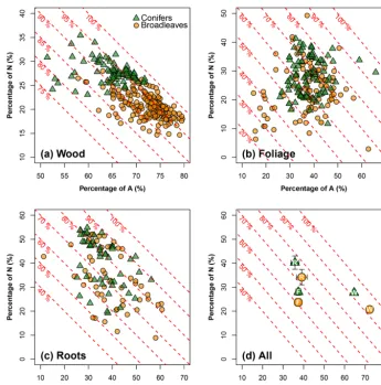
Figure 2.A meta-analysis of the carbon composition for northern temperate tree species: the xaxis represents the percentage of

acid-hydrolyzable compounds (e.g., cellulose, noted as A; in %), and theyaxis represents the percentage of non-soluble and non-hydrolyzable

compounds (e.g., lignin, noted as N; in %). The oblique red dashed lines show the sum of A and N and their values. The remaining percentage,

i.e., 100−(A+N ), refers to the portion of non-polar extractives, ethanol or dichloromethane compounds (E), and water soluble compounds

(W). Analyses are conducted(a)for wood (106 data points for broadleaves, and 79 for conifers),(b)for foliage litter (106 data points for

broadleaves, and 83 for conifers) and(c)for root litter (58 data points for broadleaves, and 49 for conifers).(d)is a statistical summary

(symbols and means and error bars – 1.96×SE) for wood (W), foliage (F) and roots (R) in a common coordinate system. Note the use of

different axis graduations in each plot. See Supplement II for the data sources.

pools corresponded to at least 75 % and, in most cases, was greater than 90 %. W and E accounted for only small per-centages of the carbon composition (Fig. 2a). Nevertheless, this dominance of A and N over W and E was much less pro-nounced in foliage and root litter types (Fig. 2b and c). Gen-erally, the different tree organs can be ranked according to the sum of the proportions of A and N as follows: woody debris (> 90 %) > roots (70 %–80 %) > foliage (60 %–70 %; Fig. 2d). The effect of tree functional type on litter carbon qual-ity strongly interacted with that of the tree organ. For wood, broadleaves and conifers had clearly shifted point clouds for the relationship between A and N carbon pools: there was a greater proportion of A and a lower proportion of N in broadleaves than in conifers. In foliage and root litter, the effect of tree functional type on the proportions of A and W was less pronounced than for wood. The main difference

be-tween broadleaves and conifers occurred in N rather than in A (Fig. 2d). Broadleaved litter had a smaller N proportion than coniferous litter, regardless of the tree organ (Fig. 2d). The proportions of A and N relative to those of E and W were quite stable between broadleaves and conifers regardless of the tree organ (Fig. 2d).

3.2 Sensitivity analyses on the impact of initial soil and litter settings on model output

and b). Next, we found that model fits were better when an observed CS to 0.4 m in depth (Fig. S3a and c) was used as the initial carbon quantity than when a CS to 1.0 m in depth was used (Fig. S3b and d). Nevertheless, it remained more advantageous to use the CS to 1.0 m observed during the first assessment as the model input because Yasso07 is calibrated to predict the CS down to 1.0 m in depth (Rantaraki et al., 2012).

Different choices of fine-root-to-foliage ratio for fine-root litter input also significantly influenced Yasso07’s perfor-mance in predicting changes in soil C (Fig. S3). Ratios of 0.1–0.8 for broadleaves and 1.8–3.0 for conifers achieved the best fits between simulated and observed changes in the soil CS according to different scenarios (Fig. S3). Using a con-stant value of 1.0 for both broadleaved and coniferous sites seems to be an acceptable compromise between the two tree functional types, even though the choice is not optimal for each functional type taken individually.

As a result of the above diagnoses, we only show fit and residual analysis results for the simulations based on the par-tial steady-state assumption, observed CS to 1.0 m and fine-root-to-foliage ratio of 1.0 (see Fig. S3d and Sect. 3.3).

Figure S4 visualized all the theoretically possible final CSs by varying initial CSs and simulated duration (from 1 to 10 000 years). Initial soil carbon quality had a pronounced impact on final soil organic CSs at the annual and decennial scales. For example, when the initial proportion of the A pool increased from 0 % to 80 %, the final proportion of A could increase by+30 to+40 tC ha−1(Fig. S4a) and the final total CSs could decrease by approximately −20 to −30 tC ha−1 (Fig. S4u) at annual and decennial scales. When simulations were performed for a millennium timescale, the initial soil carbon quality no longer impact final soil carbon quality. In other words, the same final soil carbon quality was obtained regardless of the initial soil quality (Fig. S4).

3.3 Simulated versus observed carbon data

Using only mean litter input, the theoretical CSs

(CSsteady-state) simulated from the initialization method

and the observed CSobs,t1 to 1.0 m in depth shared the same order of magnitude and were quite comparable (Fig. S5). However, the CSs were overestimated for most coniferous stands and underestimated for broadleaved stands (Fig. S5).

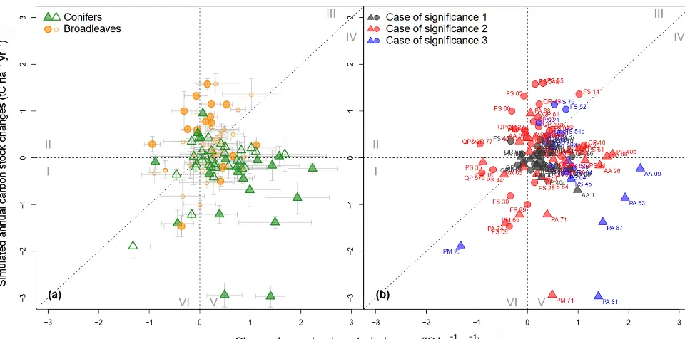
When simulated ACCs were plotted against the ob-served ones, the point clouds were distributed around the 1:1 diagonal line despite fairly high dispersion (Fig. 3). The correlation between predicted and mea-sured ACC remained weak (R2<0.1). The mean ob-served and simulated ACCs for all sites were, respec-tively,+0.34±0.06 tC ha−1yr−1(+0.20±0.06 tC ha−1yr−1 for broadleaved stands and +0.48±0.10 tC ha−1yr−1 for coniferous stands) and+0.00±0.07 tC ha−1yr−1(+0.28± 0.09 tC ha−1yr−1 for broadleaved stands and −0.28± 0.11 tC ha−1yr−1 for coniferous stands); 23 % of the

broadleaved stands and 39 % of the coniferous stands showed significant differences between observed and sim-ulated ACCs (Fig. 3a). In only approximately 17 % of the sites, ACCs were significantly different from 0 for both sim-ulated and observed results (i.e., case 3 in Fig. 3b). Here, there was a significant effect of tree functional type on the observed and simulated values. The model tended to over-estimate ACC in broadleaved stands but to underover-estimate ACC in coniferous stands. Approximately two-thirds of all the sites showed predicted and observed changes in CSs of the same trend (i.e., data points in zones I, III, IV and VI; Fig. 3), while approximately one-third of the sites were in the remaining zones (II and V) where the predicted trend was contrary to the observed trend. From the residual dis-tribution, we also found that the model where carbon quality was set with the partial steady-state assumption (Fig. 3) had a better fit than the model set with the complete steady-state assumption (Fig. S6).

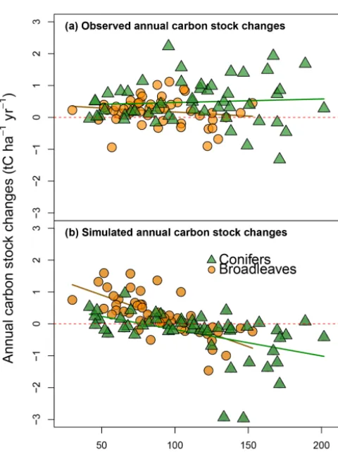
The simulated ACCs exhibited a negative linear relation-ship with the initial soil CSs (Fig. 4b), whereas this trend was not found for the observed ACCs (Fig. 4a). Storm dam-age and soil type could not clearly explain these trends in the residuals. For coniferous stands only, the residuals showed significant differences among the three major types of soil (n of sites > 5): cambisol > luvisol > podzol (Fig. S7). The coniferous stands tended to be younger than the broadleaved stands. Neither tree age nor the interaction between tree age and tree functional type had any significant effect on resid-uals. For all the sites together, the residuals became higher with increasing latitude, indicating that simulated ACCs were more overestimated in northern zones (analysis of co-variance – ANCOVA; F =11.2, P <0.001). This pattern was particularly strong for broadleaved stands (Fig. S8a). No similar trend was found for coniferous stands (Fig. S8e). Both residual signs were generally present for all of the main species (Fig. S8b, c, d, f, g and h). Broadleaved and conifer-ous stands differed in their responses to environmental fac-tors: for coniferous stands, neither temperature nor precipi-tation had much effect on residuals, while for broadleaves, precipitation was negatively correlated with residuals (AN-COVA,F =10.8,P <0.001).

Figure 3.Comparison between simulated and observed changes in annual carbon stocks (ACCs; in tC ha−1yr−1). Circles and triangles represent sites dominated by broadleaves and conifers, respectively. The partial steady-state assumption was used when initializing CS quality to 1.0 m in depth. The fine-root-to-foliage ratio for broadleaves and conifers is 1.0. To facilitate readability, Roman numerals (I–VI)

denote the six zones in which data points are distributed. In(a), error bars represent standard errors; hollow and filled points represent

non-significant and significant differences, respectively, between simulated and observed ACCs according to thettest (at a 95 % confidence

interval). In(b)the case of significance is as follows: 1 – no significant difference from 0 for either observed or simulated ACC; 2 – a

significant difference from 0 for either observed or simulated ACC; and 3 – a significant difference from 0 for both observed and simulated ACC.

4 Discussion

4.1 Agreement between simulated and observed annual changes in soil carbon stock

Testing widely popularized soil carbon models on a large dataset is highly meaningful work that enables researchers not only to assess the model’s predictive ability over vari-ous climatic and ecosystem types but also to provide lessons and implications for future modeling work. Here, compared with observed CS data to 1.0 m in soil depth from the RENECOFOR network, we found that the simulated stocks

(CSsteady-stateversus CSobs,t1) to 1.0 m showed the same

or-der of magnitude and validated Yasso07’s ability to predict average CSs at the scale of the French territory. This solid performance at the national scale supports Yasso’s aim to be generalizable and is consistent with previous studies (see Ortiz et al., 2013; Lehtonen et al., 2016; Hernández et al., 2017). Nevertheless, the observed CS to 1.0 m in depth att1

already exceeded the CSsteady-statefor most coniferous stands

(Fig. 5S), suggesting, to some extent, that the model param-eters were not adapted to the RENECOFOR dataset. Such inadaptability may simply be due to setting an overly high decomposition rate for the slow carbon pools in the model. As the coniferous stands were on average younger being

af-forested more recently than the broadleaved stands (Jonard et al., 2017), the model may also not have been able to ac-count for historic land use changes when the soil organic CS was calculated at the steady state. Figure S5 shows that for most broadleaved stands, observed stocks were lower than their CSsteady-state, possibly indicating that steady-state

equi-librium had not yet been reached at these sites.

re-Figure 4. Observed (y axis;a) and simulated annual changes in

carbon stocks (yaxis;b) plotted against the CSs observed to 1.0 m

in depth (xaxis) during the first soil CS assessment. Regressions

are as follows:y= −0.003x+0.422 (R2=0.03) for observed

val-ues at the sites dominated by broadleaves, y=0.001x+0.353

(R2=0.01) for observed values at the sites dominated by conifers,

y= −0.016x+1.715 (R2=0.62) for simulated values for the sites

dominated by broadleaves andy= −0.008x+0.648 (R2=0.60)

for simulated values for the sites dominated by conifers.

produce this observed effect of tree functional type on ACC, as the model does not take into account changes in land use history, as for the case of steady-state CSs mentioned above. Except for tree functional type and geographical location (e.g., latitude, which is correlated with climatic variables), qualitative ecological variables that are assumed to be key factors influencing carbon sequestration processes (e.g., soil type – except for coniferous stands, storm damage and stand age range) showed limited ability to explain residuals. Note that these factors were not fully crossed for the 101 sites, making it difficult to test each single factor.

Simulated ACCs showed a strongly negative correlation with the observed initial soil CSs (CSobs,t1), with an overes-timation of ACC at sites with lower CSobs,t1and an underes-timation at sites with higher CSobs,t1(Figs. 4 and S9). This is logical in view of the model’s inherent mechanism. With

in-creasing initial CS, there is an increase in the quantity of the easily decomposable compounds in the soil, i.e., A, W and E, which triggers a more substantial mass loss at a decennial scale. However, the data on observed changes in CSs did not support this trend.

Several quantitative soil physical and chemical properties showed clear correlations (especially for broadleaved stands) with ACC residuals (Fig. 5). Also, in the principle compo-nent analyses (Fig. S9), the arrows representing soil vari-ables are slightly closer to the pivoting axis of “initial CS and ACC residuals” than those representing climatic and ge-ographic variables, notably for broadleaved stands. These results highlight the potential interest of incorporating soil properties into new versions of the Yasso model, which cur-rently lacks, or only implicitly incorporates, soil parameters. Indeed, there is considerable evidence that soil physical and chemical properties can greatly influence soil carbon dynam-ics and storage capacity (Beare et al., 2014; Dignac et al., 2017; Rasmussen et al., 2018).

Despite Yasso07’s significant prediction bias at a number of sites, it is unreasonable to simply attribute the bias to the model per se, since multiple uncertainties affecting the qual-ity of the model’s input data can be identified (see Sect. 4.2– 4.3). These uncertainties can occur not only with Yasso07 but also with other prevailing models, highlighting large knowl-edge gaps in ecology and soil carbon modeling.

4.2 Setting soil carbon quality for model initialization: a recurrent challenge in soil carbon modeling Great uncertainty is associated with model initialization in terms of soil carbon quality, as it is usually estimated, not measured, for example, through matrix inversion with the as-sumption that the litter input has been the same for decades. Compared to measuring total soil CSs, measuring soil carbon quality is much more labor-intensive and time-consuming. Moreover, soil carbon quality data from different sources may be partly or totally incompatible due to the use of dif-ferent chemical pools or fractionation protocols (Blair et al., 1995). Therefore, measured data for soil carbon quality are generally lacking at the worldwide scale. This lack of infor-mation is a recurrent issue for soil carbon dynamics mod-eling (see Elliot et al., 1996, who have discussed the issue of “measuring the modelable”). Many prevailing soil carbon models require setting carbon quality in addition to carbon quantity, e.g., Romul (Chertov et al., 2001), RothC (Cole-man and Jenkinson, 1996), CENTURY versions (Parton et al., 1987; Metherell et al., 1993) and CBM-CFS3 (Kurz et al., 2009). Setting carbon quality in models inappropriately may greatly change CS predictions (Wutzler and Reichstein, 2007; Carvalhais et al., 2008, 2010).

Figure 5.Residuals of annual carbon stock change (ACC) plotted against selected soil physical and chemical properties. Top plots with green triangles represent sites dominated by conifers, and bottom plots with orange dots represent sites dominated by broadleaves. Regressions in

all five subplots for the broadleaved sites(b, d, f, h, j)and in one subplot for the stands dominated by conifers(a)are significant (∗P <0.5).

See Table S2 for linear regression results for all 11 soil variables. Red dashed line indicates the zero line.

assumption, the partial steady-state assumption made it pos-sible to account for slow-cycling pools, which could still be accumulating carbon, and fast cycling pools in equilibrium (Wutzler and Reichstein, 2007). We did not use the precise method proposed by Wutzler and Reichstein (2007) to esti-mate initial carbon quality due to a lack of information nec-essary for the decomposition–accumulation dynamics of the H pool. Instead, while we followed the same partial steady-state assumption, we revised the proportions of the N and H pools and assumed that the A, W and E pools were in equi-librium and equal to the simulated values. We also assumed that the sum of all pools att1was equal to the observed stock.

We found that our partial steady-state assumption gave rise to generally better model fits than the complete steady-state assumption (Fig. S3; see also Figs. 3 and S6), indicating its good suitability to the RENECOFOR sites. When plotting

CSstead-stateagainst CSobs(Fig. S5), we found a discrepancy:

while the CSobs values of most of the broadleaved stands

were smaller than CSstead-state, the CSobsof most of the

conif-erous stands were greater than CSstead-state. This discrepancy

was brought into the ACC fit when the complete steady-state assumption was adopted (Fig. S6). Nevertheless, the partial steady-state assumption can, to some extent, mitigate such a discrepancy. For broadleaved stands, the revised propor-tions of the A+W+E pools became higher than those at the complete steady state (Fig. 6; with 70 % of stands above the steady-state line), thus reducing the model’s overestima-tion of ACC. For coniferous sites, the proporoverestima-tions of the A+W+E pools were often compressed (Fig. 6; with < 50 % of the stands above the steady-state strip), thus reducing the model’s underestimation of ACC at the steady state.

For future work, it would definitely be worthwhile to com-pare both assumptions for several prevailing carbon models (e.g., Yasso07, RothC, Century, etc.), as studies comparing

Figure 6.Distribution of estimated carbon quality based on the par-tial steady-state assumption (box plots) versus those based on the complete steady-state assumption (whose ranges are all very nar-row and are expressed with strips in color: 13 %–15 % for the sum of A, W and E – cyan; 49 %–53 % for N – brown; and 33 %–36 % for H – purple). For each box plot, the low and top edges of the box correspond to the 25th and 75th percentile data points, respectively; the line inside the box represents the median, and there are no out-lier points in this case. Br. – broadleaved stands; Co. – coniferous stands.

initialization assumptions still remain scarce compared to those on model comparisons.

pos-sible chemical-pool compositions. This sensitivity analysis confirmed the high influence of initial soil carbon quality on soil CS estimates (Fig. S4), notably at short temporal scales (i.e., yearly and decennial). This result is in line with pre-vious CS modeling studies (Parton et al., 1993; Kelly et al., 1997; Smith et al., 2009; Foereid et al., 2012), confirming that initialization is a crucial step for all chemical-pool-based carbon models. Our sensitivity analysis further showed that the effect of initial CS composition would gradually vanish with increasing length of time, especially in the case of sev-eral centuries or millennia. Our analysis provides new in-sights on the sensitivity of CS estimates to the method and assumptions used in model initialization. This analysis can be transposed to other carbon models to test their theoretical performance and robustness at different temporal scales and to compare models.

Finally, testing different initialization assumptions and performing sensitivity analyses are not enough to solve the predictability issues related to uncertainties in soil carbon quality. Based on ground truth data, Balesdent et al. (2018) showed that carbon age strongly reflects soil depth and ecosystem type. It appears to be highly necessary for future modeling work to capture better indicators of carbon stabi-lization mechanisms in the model initiastabi-lization procedure. Yasso07’s particular model configuration, i.e., based on surable chemical pools, may make it possible to use mea-sured soil carbon quality data for model initialization instead of steady-state assumptions. Future measurements of radio-carbon age for soil organic matter at the RENECOFOR sites may offer an ideal opportunity to compare the impact of ini-tial soil carbon quality on Yasso07’s predictions.

4.3 A precise estimation of root litter quantity helps improve Yasso07 predictions

An important source of uncertainty in the estimates of litter quantity at the RENECOFOR sites concerned fine-root litter input. Many studies have revealed that fine roots are a ma-jor source contributing to total litter quantity due to their fast turnover rates (Brunner et al., 2013; Kögel-Knabner et al., 2002; Berg and McClaugherty, 2008). In some forest ecosys-tems, the proportion of fine-root litter is even comparable to that of foliage (Freschet et al., 2013; Xia et al., 2015). However, estimating fine-root litter input is, again, a time-consuming and challenging task. For this reason, to our best knowledge, probably no nationwide forest inventory projects have ever incorporated direct measurements of the dynam-ics of fine-root litter input (and this information is also lack-ing for the RENECOFOR network). Fine root turnover for forest species varies depending on climate, tree species and management scenarios (Kögel-Knabner et al., 2002; Litton et al., 2003; Mokany et al., 2006), and this makes choosing model input values highly subjective and difficult. By test-ing variable fine-root-to-foliage ratios of litter input, we ob-served a significant shift in the ACCs predicted by Yasso07

(Fig. S3). This finding not only highlights the importance of precisely quantifying fine-root litter input but also sug-gests that broadleaves and conifers may have a different fine-root litter input ratio with regard to that of foliage, although we chose the same ratio for both broadleaved and conifer-ous stands in this study. It should be noted that using one ratio per tree functional type (conifers versus broadleaves) can only change the overall prediction baseline and cannot reduce data dispersion. Consequently, it is of great interest to estimate fine-root litter input quantity at the species level through direct measurements and then couple the specific data with Yasso07.

Potentially important litter input may also come from the shrubby and herbaceous understory species, which we did not take into account in this study due to data unavailabil-ity. The herb and shrub layers are typically not included in forest inventories, though they can contribute significantly to the annual litter production in forests (e.g., de Wit et al., 2006; Gilliam, 2007; Lehtonen et al., 2016). Muukkonen and Mäkipää (2006) estimated that the carbon input from herba-ceous and shrub vegetation in Finnish forests was from 0.50 to 0.66 tC ha−1yr−1. This is quite high, as the value repre-sents of the mean total tree litter input for all the RENECO-FOR sites combined (Table 1). This is in line with data from Didion et al. (2018), who estimated that understory vegeta-tion at the sites of the Swiss Navegeta-tional Forest Inventory con-tributed on average 10 %–15 % to the total observed annual non-woody carbon turnover with a range from a few percent to more than 50 %.

Finally, Yasso07’s parameter set was calibrated based on one of the richest litterbag datasets in the world in terms of number of observations. The state of the art of soil car-bon modeling assumes that litter input and decomposition processes are the driving forces in soil carbon accumulation. However, other important sources of biological carbon input exist, e.g., soil fauna and rhizodeposition; unfortunately, our ability to take them into account in modeling processes re-mains poor. Whether, and to what extent, the bias found in our Yasso07 results is related to these alternative sources of biological carbon input is unknown.

4.4 Suggestions for future modeling improvements First, we found the Yasso07 model structure and algorithm solid, clear and simple to operate, in agreement with the pos-itive remarks in the literature (Rantakari et al., 2012; Didion et al., 2014; Lu et al., 2015; Wu et al., 2015). Regarding its mass flow parameters, Fig. S1 only shows the mass flows that are statistically significant in the case of the Tuomi (2011) pa-rameter set. Yasso07 keeps all the theoretical mass flow pos-sibilities in theApmatrix in (Eq. 1b). However, a mass flow

This quantity is disputable in light of soil biochemistry, be-cause lignin, the major component constituting the N carbon pool, is not likely to pass into the A pool but would instead probably condense with other nearby phenols, peptides or saccharides (Burns et al., 2013).

As a model for predicting soil carbon dynamics, Yasso07 is still overly simple in the description of some soil variables that are known to strongly impact decomposition processes. For example, soil mineralogy or aggregation is yet to be ac-counted for in Yasso07. Indeed, the model has often been applied on soils fairly rich in organic matter (e.g., Karhu et al., 2011), where the consideration of soil mineral properties was not particularly relevant and where the authors’ assump-tion that litter quantity is a good proxy for soil properties was reasonable. In addition, when Yasso, Yasso07’s proto-type, was published in 2005 (Liski et al., 2005), information on mineral soil properties in the various forest soil horizons was not commonly available. Nowadays, however, it is easier to obtain, although there is still not enough detailed data for consistent application across large regions or at the national scale (Didion et al., 2016).

5 Conclusions

We tested the performance of the Yasso07 soil carbon model on decennial-scale French nationwide forest data collected through the RENECOFOR network. We also compiled a meta-analysis database for litter carbon quality and carried out sensitivity analyses to characterize the effect of initial litter input and soil carbon quality on the model’s predic-tions. We showed that, while the model’s estimates of CS to 1.0 m in depth and of ACC stayed within the same or-der of magnitude as observed values, the accordance between the observed and simulated ACCs at the site scale remained weak. There was a bias in the model’s predicted trends for changes in CS at more than one-third of the French sites. As we have shown for Yasso07, the performance of soil carbon models should be examined before their application to man-agement guidelines and policymaking for forest ecosystems at any scales.

Biases can be attributed to multiple factors concerning model input, such as (i) uncertainty in the measurement data for soil CSs and changes, (ii) a lack of information on initial soil carbon quality at the site level, and (iii) a lack of infor-mation on below-ground litter production. These factors are valid for the state-of-the-art soil carbon modeling, regardless of the model that one uses. Our sensitivity analyses explicitly confirmed the importance of factors (i) and (ii) above. Ap-propriately setting soil carbon quality is one of the most cru-cial steps to guarantee the model’s fit. We found that the par-tial steady-state assumption gives rise to a significantly bet-ter model fit than does the complete steady-state assumption, when setting soil carbon quality. Some of the model’s param-eters governing the transfer among soil pools are statistically

derived and not directly measured and thus may poorly rep-resent actual biochemical decomposition processes. Residual analysis also suggests a potentially important role of physi-cal and chemiphysi-cal soil properties in explaining the model’s prediction ability.

Our findings allow us to provide modelers, users and poli-cymakers with the following suggestions:

– We suggest that Yasso07 modelers keep the current model structure, algorithm and parameters but incorpo-rate some more refined biochemical processes: for ex-ample, that they (i) revise certain mass flows to achieve both statistically and biologically meaningful processes (especially the N→A flow), (ii) refine the decompo-sition process (i.e., the residence times between the A, W and E soil carbon pools); and, possibly, (iii) explic-itly incorporate easily measured soil parameters to bet-ter represent biophysical and biochemical inbet-teractions in soil carbon cycling.

– We suggest that Yasso07 users work in conjunction with modelers in order to better reduce the uncertainties in model initialization for soil CSs. We also suggest mea-suring forest carbon quality and quantity and below-ground fine-root litter to better feed the model.

– We suggest that policymakers remain prudent toward diagnoses based on a single carbon model, especially when a long-term trend is predicted. Predictions from multiple models should be cross-validated for both global and local areas.

This study, involving decennial observations at sites spread over a large spatial scale and covering different ecosystems, provides a good opportunity to facilitate future model calibration, improvement and reassessment. Finally, with Yasso07 as an example, this work highlighted the bot-tleneck in soil carbon modeling caused by the lack of knowl-edge or data on soil and litter carbon quality and on fine-root litter quantity, which creates high uncertainties for model ini-tialization. Simultaneously, we demonstrated methodologies for testing other soil carbon models via sensitivity analyses to better enable us to understand the limits of the model and of the input data and to plan future improvements in soil organic carbon modeling. In this study, we used the model structure and parameters published in Tuomi et al. (2011a) without any modifications. Further work on sensitivity analyses incorpo-rating modifications in both the carbon quality and litter in-put settings and Yasso07’s configuration and parameters is needed to confirm the reliability of the current diagnoses.

Data availability. The plant and soil data used for model fit and

Appendix A: Nomenclature and abbreviations

Name Meaning

Carbon stock (CS) Quantity of organic carbon stocked in the soil (in tC ha−1)

Carbon stock change Increment (positive value) or decrement (negative value) of organic carbon stocked in the soil between yeart1and yeart2(in tC ha−1)

Annual carbon stock change (ACC)

Change in CSs per year (in tC ha−1yr−1)

Carbon pools The Yasso07 model contains a series of organic compounds involved in decomposition processes differing in solubility and mean residence time: water soluble compounds (W), acid-hydrolyzable compounds (A), non-polar solvent, ethanol or dichloromethane compounds (E), and non-soluble and non-hydrolyzable compounds (N). For soil, there is an additional recalcitrant pool called “hu-mus” (H). Note that in this paper, “N” only denotes non-soluble and non-hydrolyzable compounds; nitrogen is spelled in full when mentioned.

Coarse woody litter Litter originating from either coarse above-ground residues due to either harvests or storms (includ-ing coarse branches of > 4 cm in diameter and miscellaneous residues) and coarse roots of >5 mm in diameter

Fine non-woody lit-ter

Litter originating from either natural above-ground litterfall (leaves, small branches) or fine-root activities

Litter carbon quality Litter carbon (in %) belonging to the A, W, E and N carbon pools (see “carbon pools” above) Litter quantity Annual litter accumulation (in tC ha−1yr−1)

Supplement. The supplement related to this article is available online at: https://doi.org/10.5194/bg-16-1955-2019-supplement.

Author contributions. DD, MD and LSA designed the study as well

as the structure of the paper. ZM, MD, MN and LSA collected or provided the data. JL provided technical help for model use. ZM performed model simulation, data analysis and wrote the first draft. DD, MD, TE and LSA participated in data analysis and result inter-pretation. All the co-authors participated in paper preparation.

Competing interests. The authors declare that they have no conflict of interest.

Acknowledgements. This study was funded by the French Agence

de l’Environnement et de la Maîtrise de l’Energie (ADEME; con-tract reference: 14-60-C0082). The UR1138 BEF and this study were supported by a grant overseen by the French National Re-search Agency (ANR) as part of the “Investissements d’Avenir” program (ANR-11-LABX-0002-01, Laboratory of Excellence AR-BRE) – QLSPIMS project. This study is an outcome of a project en-titled “Input to improve the comparability in MRV across EU MS” within the LULUCF MRV project “Analysis of and proposals for enhancing Monitoring, Reporting and Verification (MRV) of land use, land use change and forestry (LULUCF) in the EU” funded by the European Commission. Funding for Markus Didion was pro-vided by the Swiss Federal Office for the Environment. We thank several French colleagues, Isabelle Feix (ADEME), Arnaud Legout (INRA) and Bertrand Guenet (CNRS), for their valuable comments. We are also grateful to Anna Repo (FEI – SYKE) and Emmi Hi-lasvuori (FEI – SYKE) for their explanations of Yasso07 and to Vic-toria Moore for her thorough review and suggestions for improving the English language.

Review statement. This paper was edited by Luo Yu and reviewed

by Thomas Wutzler and one anonymous referee.

References

Aber, J. D., Melillo, J. M., and McClaugherty, C. A.: Predict-ing long-term patterns of mass loss, nitrogen dynamics, and soil organic matter formation from initial fine litter chemistry in temperate forest ecosystems, Can. J. Bot., 68, 2201–2208, https://doi.org/10.1139/b90-287, 1990.

Aulen, M., Shipley, B., and Bradley, R.: Prediction of in situ root decomposition rates in an interspecific context from chem-ical and morphologchem-ical traits, Ann. Bot.-London, 109, 287–297, https://doi.org/10.1093/aob/mcr259, 2011.

Balesdent, J., Basile-Doelsch, I., Chadoeuf, J., Cornu, S., Der-rien, D., Fekiacova, Z., and Hatté, C.: Atmosphere–soil car-bon transfer as a function of soil depth, Nature, 559, 599–602, https://doi.org/10.1038/s41586-018-0328-3, 2018.

Beare, M., McNeill, S., Curtin, D., Parfitt, R., Jones, H., Dodd, M., and Sharp, J: Estimating the organic carbon stabilisation capacity

and saturation deficit of soils: a New Zealand case study, Bio-geochemistry, 120, 71–87, https://doi.org/10.1007/s10533-014-9982-1, 2014.

Berg, B. and McClaugherty, C.: Plant litter: decomposition, humus formation, carbon sequestration, 2nd Edn., Springer-Verlag Hei-delberg Berlin, 286 pp., https://doi.org/10.5860/choice.51-6172, 2008.

Brunner, I., Bakker, M. R., Björk, R. G., Hirano, Y., Lukac, M., Aranda, X., Børja, I., Eldhuset, T. D., Helmisaari, H. S., Jourdan, C., Konôpka, B., López, B. C., Miguel Pérez, C., Persson, H., and Ostonen, I.: Fine-root turnover rates of European forests re-visited: an analysis of data from sequential coring and ingrowth cores, Plant Soil, 362, 357–372, https://doi.org/10.1007/s11104-012-1313-5, 2013.

Burns, R. G., DeForest, J. L., Marxsen, J., Sinsabaugh, R. L., Stromberger, M. E., Wallenstein, M. D., Weintraub, M. N., and Zoppini, A.: Soil enzymes in a changing environment: current knowledge and future directions, Soil Biol. Biochem., 58, 216– 234, https://doi.org/10.1016/j.soilbio.2012.11.009, 2013. Carvalhais, N., Reichstein, M., Seixas, J., Collatz, G. J., Pereira, J.

S., Berbigier, P., Carrara, A., Granier, A., Montagnani, L., Papale, D., and Rambal, S.: Implications of the carbon cycle steady state assumption for biogeochemical modeling performance and in-verse parameter retrieval, Global Biogeochem. Cy., 22, GB2007, https://doi.org/10.1029/2007gb003033, 2008.

Carvalhais, N., Reichstein, M., Ciais, P., Collatz, G.J., Ma-hecha, M.D., Montagnani, L., Papale, D., Rambal, S., and Seixas, J.: Identification of vegetation and soil carbon pools out of equilibrium in a process model via eddy covariance and biometric constraints, Glob. Change Biol., 16, 2813–2829, https://doi.org/10.1111/j.1365-2486.2010.02173.x, 2010. Chertov, O. G., Komarov, A. S., Nadporozhskaya, M., Bykhovets,

S. S., and Zudin, S. L.: ROMUL – a model of forest soil organic matter dynamics as a substantial tool for forest ecosystem model-ing, Ecol. Model., 138, 289–308, https://doi.org/10.1016/s0304-3800(00)00409-9, 2001.

Coleman, K. and Jenkinson, D. S.: RothC-26.3 – A Model for the turnover of carbon in soil, in: Evaluation of Soil organic matter models, Using Existing Long-Term Datasets, edited by: Powlson, D. S., Smith, P., and Smith, J. U., Springer-Verlag, Heidelberg, 237–246, https://doi.org/10.1007/978-3-642-61094-3_17, 1996.

Didion, M., Frey, B., Rogiers, N., and Thürig, E.: Validating tree litter decomposition in the Yasso07 carbon model, Ecol. Model., 291, 58–68, https://doi.org/10.1016/j.ecolmodel.2014.07.028, 2014.

Didion, M., Blujdea, V., Grassi, G., Hernández, L., Jandl, R., Kriiska, K., Lehtonen, A., and, Saint-André, L.: Mod-els for reporting forest litter and soil C pools in

na-tional greenhouse gas inventories: methodological

con-siderations and requirements, Carbon Manag., 7, 1–14, https://doi.org/10.1080/17583004.2016.1166457, 2016. Didion, M., Baume, M., Giudici, F., and Schneuwly, J.:

Herb layer biomass in Swiss forests. 53 pages. Swiss

Federal Research Institute WSL, Biirmensdorf (ZH),

https://doi.org/10.16904/envidat.52, 2018.