Procurement and Pricing Decision for Trapezoidal Demand Rate and Time Dependent Deterioration

(1)

International Journal of Innovative Technology and Exploring Engineering (IJITEE) ISSN: 2278-3075,Volume-8 Issue-12, October 2019

Procurement and Pricing Decision for Trapezoidal

Demand Rate and Time Dependent Deterioration



Jitendra Kaushik, Ashish Sharma

Abstract:Deterioration rate may be constant or varies with time. In real life time dependent deterioration is observed in many products like fruits, bakery products, milk products etc. Generally deterioration rate increases as the time passes. In this paper we present an inventory model for the trapezoidal type demand function and time dependent deterioration rate. Demand rate depends on time as well as price. Shortages are allowed with partial backlogging. In order to illustrate solution procedure numerical examples and sensitivity analysis have been demonstrated.

Keywords: Inventory model, Trapezoidal type demand, deteriorating items, price and time dependent demand

I. INTRODUCTION

In recent years, inventory model for deteriorating items gets focus of many researchers. Deteriorating items having more importance due to high margin which also results high loss associated with them. In real life deterioration is a natural phenomenon which can be defined as a process of becoming impaired or inferior in quality from being used for its original purpose. It is quite essential for the consideration of deterioration rate in the analysis of items like fruits, vegetables, perfumes, pharmaceutical, radioactive substances etc.. With a view to address this research problem and provide pragmatic solution on offer several inventory models have been developed in the past. These models began with classical inventory model [24]-[25] these studies explicitly states that depletion of inventory model is primarily due to constant demand rate. Effects of deterioration on fashion products after their prescribed dates were studied by [26]-[27]. [1] established no shortage inventory model for deteriorating items with constant demand rate and constant deterioration rate. Similarly [2] considered classical Economic Order Quantity (EOQ) model with linearly deterministic demand rate. Since then, many researchers have exploited deteriorating model with time varying demand, presuming various assumptions for example[3]-[6] and [3] examined the non-shortage inventory model with a linear dependent on time trend in demand whereas [4]

Revised Manuscript Received on October 05, 2019.

Jitendra Kaushik, Department of Master of Business Administration and PGDM, Sunstone Eduversity, Lower Ground, 006 Spring House, Grand Mall, MG Road Gurugram, Haryana 122002, INDIA,. AND, Department of Mathematics, Institute of Applied sciences and Humanities, GLA University, NH-2, Mathura-281406, INDIA. Email: jitendrakaushik1986@gmail.com

Ashish Sharma, Department of Mathematics, Institute of Applied sciences and Humanities, GLA University, NH-2, Mathura-281406, INDIA. Email: ashishsharma@gla.ac.in

considered EOQ model with constant deterioration and demand rate changes linearly. [6] Developed Lot size inventory models with continuous time varying demand under three replenishment policies for deteriorating items.

However, most of the above cited studies have utilized inventory model with linearly or exponentially, increasing or decreasing demand rate, which limits applicability of these model in real life, as demand for item cannot increase linearly. [7] Was the pioneer researcher to demonstrate inventory model with ramp type demand function, which is much practical in real life as demand linearly increases in the beginning and become constant in second stage when market gets stable. Afterwards [8] considered deterministic and probabilistic demand situation with ramp type demand function of time for the deteriorating items. Study by [9] introduced two possible shortage models (i.e. model starting with no shortage and model starting with shortage) with ramp type demand function of time for the deteriorating items. [10] presented an inventory model with ramp type demand function which depends on time and deterioration rate follows Weibull distribution with partial backlogging. Recently [23] adopted ramp type demand to upstream and downstream trade credit finance with consideration of minimum cost at per unit of time. [22] Presented deterministic inventory model with seasonal demand is price and time dependent and shortage allowed with partial backlogging.

In this paper we have developed an inventory model with time dependent deterioration rate, shortage allowed with partial backlogging presuming trapezoidal type demand function with infinite replenishment. Three phases of trapezoidal demand function has been adopted with three different price and time dependent demand functions. During shortage, number of customer decrease as waiting time increases. Graphical analysis approach used to show concavity of profit function with respect to decision variables. Trapezoidal type demand function consists with three stages, in first stage demand increases then it reached to saturation in second stage in last demand rate decreases. This demand pattern is commonly observed in fruits, vegetables, sea foods items etc. Such model was firstly studied by [17] and [18] who proposed an Inventory model where deterioration rate is time dependent, with trapezoidal type demand and partial backlogging is allowed in the model.

(2)

model for Weibull-distributed deteriorating items with trapezoidal type demand where shortage are allowed. [21] Consider inventory model for perishable items with Quadratic trapezoidal demand rate under constant deterioration and partial backlogging.

To this end, the paper is presented in the following manner, notations and assumptions of the model are presented. In section 3 analysis of the model is presented. Section 4 contains mathematical solution procedure and numerical analysis. Section 5 contains the sensitivity analysis at different segments and lastly article end with vivid concluding remarks.

II. NOTATIONS AND ASSUMPTIONS

In this model we considered price and time depended on demand function under the presence of constant deterioration. The demand function is linear in time and power function in price. Inventory once restore will use in one complete demand season. There are three possibilities that inventory will deplete either in phase 1, 2 or 3. All three situations are discussed in three cases. After getting the optimal profit for all the three cases we will select the maximum. This will give the overall optimum value of the profit function. Shortages are allowed and partially backlogged since we assume that the probability of purchasing the item by a customer will decrease with the increase of the waiting time. We provide a discounted price to loyal customers for those who are waiting up to the next replenishment. In this inventory model, we are using the following notations

1.1. Notations

T: Interval length

T1: Time up to which demand increases.

T2: Time up to which demand remains constant and then decreases.

TLF: Time epoch at which inventory depletes and shortages start. F =1, 2 and 3 (Decision variable)

I: Initial Inventory level Ib: backlogged shortage C0: ordering cost

C1: holding cost, per unit per unit time C: purchase price per unit

θt: time dependent deterioration rate

P: Per unit selling price of item. (Decision variable) λP : backlogged price ; (0 < λ < 1)

1.2. Demand function

We consider a price and time-dependent iso-elastic demand function with constant deterioration rate. Demand is a linear function of time and a power function of price. For three different phases, three demand functions are defined as follows:

For phase I:

 

, 1

a bt f P t

j P



 ; 0 ≤ t ≤ T1

For phase II: ₂

 

, 1

j

a bT f P t

P



 ; T1 ≤ t ≤ T2

For phase III: ₃

 

, j

a bt

f P t r

P



  ; T2 ≤ t ≤ T

Here a, b and j are the constant demand parameters. Parameter ‗r‘ provides the flexibility that the demand in the third phase may start with a jump.

1.3. Assumption

Following are the main assumptions of the presented model

(1) The probability that the customer waits during the shortage depends up on the waiting time, as waiting time increases the probability that the customer will wait up to the next replenishment decreases

( ) 1 ( /T) ; 0 T

       

(2) Backorder price is



P

such that

C





P

< P

for this

1 C

P

 



(3) Demand function is positive;

f

F

(P, T)



0

(4) Selling price per unit should be greater than purchasing price and the total holding costP C + TC₁. The RHS of the expression is known as price floor.

(5) Replenishment rate is infinite. (6) Demand decrease as price increase

(7) Backlogs may clear at arrival of next replenishment and shortage time cannot be exceed the length T

III. ANALYSIS

In this model, we have three different cases according to the depletion of inventory in the growth, constant and decline phase

Case 1: Inventory depletes in growth phase (0 ≤ TL1 ≤ T1)

Holding cost is given by

1

1 1[ {(TL1 0) f (P, t)1 }dt]

0

L

T

H C   t

The revenue earned

1

1 1 1

0

( , )

L

T

b

R





Pf P t dt





PI

Here Ib1 is the backlogged amount is given by

1 2

1 1 1 2 2

1 1

3

2

(P, t) (T t) dt + (P, t) (T t) dt

+ ( (P, t) r) (T t) dt b

L

T T

I f f

T T

T f T

 



 _  _ 

 



The initial inventory level is

1

{ ( , ) }

1 1

0 T_L

I   f p t  t dt

Profit per unit time for the first stage

Net1 = (R1 – H1 - C0 – C (I1 + Ib1)) / T (1)

Case 2: Inventory depletes in constant phase (T1 ≤ TL2 ≤ T2)

(3)

1

2

1

2 1 1 1

0

L 2 2

[ {(T 0) f (P, t) }dt

+ {(T 0) f (P, t) }dt ]

L

T

H C t

t       



R2 the revenue earned

1 2

1

2 1 2 b 2

0

f (P, t) dt f (P, t) dt PI

L

T T

T

R 



P 



P 

Here backlogged amount is

2

2 2

2 2(P, t) (T2 t) dt + ( 3(P, t) r) (T t) dt

L

T T

b

T T

I 



f  



f   

And the initial inventory level is

1 2

1

2 1 2

0

{ ( , ) } { ( , ) }

L

T T

T

I 



f p t  t dt



f p t  t dt

Profit per unit time for the Second stage

Net2 = (R2 – H2 - C0 – C (I2 + Ib2) ) / T (2)

Case 3: Inventory depletes in decreasing phase (T2 ≤ TL3 ≤ T)

Holding cost is given by

1 2

1

3

2

3 1 1 1 2 2

0

3 3

[ {(T 0) f (P, t) }dt + {(T 0) f (P, t) }dt

+ {(T 0) f (P, t) }dt]

L T T T T L T

H C t t

t          



The revenue earned is

3

1 2

3 1 2 3 b3

0

f (P, t) dt f (P, t) dt (f (P, t) r) dt + PI

L

T

T T

R 



P 



P 



P  

Here backlogged amount is

3

3 ( 3(P, t) r) * (T t) dt

L

T

b T

I 



f   

Profit per unit time for the third stage

Net3 = (R3 - H3 - C0 - C (I + Ib3)) / T (3)

Now we discuss the concavity of the profit function NetF with

respect to the decision variables TLF.

Theorem 1: (a)Net1 is concave function in TL1. (b)Net2 is concave function in TL2.

(c) Net3 is concave function in TL3 if

( 4 ) ( 2 )

1 1 3

[1 ( ₃ )]

( ) ( ) ( 2 )

1 1 2 1 1

C a T P r T a T

j

P r C T

C r T a T C b b C P T

                   (4)

Proof: (a) On partially differentiating Net1from expression (1) with respect to TL1 , we get

( ( ₁ ₁(C P C_{1 1}) ₁ ) _{1 1}( ( _{1 1})

( ( ) )))

1 1 1 1 1

1 3

j j

P a CT T T PT T T P C C T

b CT T C P C T PT T T                   (5)















1



1 1 1 1

1 3

2 ( )

2 2

j

j T P C C a C T C P

P

b T C P C T T C P T T

T  



 _     _

      

  ₍₆₎

Now the rhs of the above expression is

2

1 1 1 1

{ ( ( ) (2 ( ) (2 )}

( 2)

j j

j

T P b C P T C P b P aC

P C a P





 _ _ _ _{ } _

   

Thus on simplification

2

{ (₁ ( ) ₁ (2 ₁( ) (2 ₁)}

0

( 2)

j j

T P b C P T C P b P aC

j

P C a P

  



 _ _ _ _{ } _



  

Since C < Pλ therefore the above expression is negative.

Thus Net1 is a concave function with respect to TL1

(b) On partially differentiating Net2 from expression (2) with respect to TL2, we get

( ₂ ₁( ₁( ₁ ₁))

( ( ) ( )

2 1 1 1 1 1

( ( ) ( )

1 2 1 1 1 1 1

( ( ) ( )))

2 1 2 1 1 1 1 1

2 3 2

j j

P T P T C C T T a T C T C P C T T C P bT T C T C P C T T C P Net bT T C T C P C T T C P

T T T_L                                  (7)

2 1 1 1 1

2

2 2 1 1 2 1

2

2 3 2

( ( 2 )

( ) bT ( ))

j j

L

P T P C T C C T

Net a C T C P C T C P

T T T     _  _ _          (8) The RHS of the above expression is

2 1 1 1 1 1 1 1 1

[ { ( 2 ) ( )} ( )]

( )

j

T P C T C C T C a bT bT C T P P a C P

 



       

(4)

2 1 1 1 1 1 1 1 1

[ { ( 2 ) ( )} ( )]

0

( )

j

T P C T C C T C a bT bT C T P P a C P

 



        _

 

Since

C





P

therefore the above expression is negative

(c) On partially differentiating Net3 from expression (3) with respect to TL3, we get

1 2

3 1 1 1 1 1

2

1 1 1 1

2 1 1 1 1 1

3 2 1 1 1 1

2 3 ( ( ( ( ) ( ( ) ( )( ) ( ( ) ( )))

j j j

j j

P T P r bPT C P rT bC T

C P T C bT P r T

T C bT P r T T P r bT C P

a T C T C P C T T C P

T





 _ _  _ _ _                    (9)

3 1 3

3 1 2 1

2

3 3 2 1 1 1 1

2 2

3 3

( ( ) ( ( )

( 2 ) Pr )

( ( 2 2 ( )))

j j

L

P a C T C P P C r T T C r T T

Net b T C T C P C T T C P

T T        _ _ _  _{ }              (10) The RHS of the expression (9) is negative iff

3 1 3

3 1 2 3 1 3 1 1

3 2 3 1 3 1 1 3 1 1

P [(aC-aT C -aP ) P (-Cr+T r ) +T C r-T T C +T C T +Pr )

+b(T C-T T C -T P+2C T T -2T C+2T P )< P

j j j        _ That is

3 1 3 3 1 2 3 1

3 1 1 3 2 3 1 3

1 3 1 1

aC-aT C -aP +P Cr-P T r +T C r-T T C +T C T +Pr +bT C-bT T C -bT P

+2T bT -2T C+2T P < P j j j        On simplification

1 1 3 3 1 1

2 3 1 3 1

(aC-4T C) +P (r+2T -a)+P r(C-T )+T C (r+T -a)

-T T C ( -b)+bT (C-P+2T ) < P j

j





Implies that

1 1 3 1 1 2 1 1

3

( 4 ) ( 2 ) [ ( ) ( ) ( 2 ]

[1j ( )]

C a T P r T a T C r T a T C b b C P T P r C T

  



           

  

Thus

( 4 ₁) ( 2 ₁ ) ₃

[1 ( ₃ )]

( ) ( ) ( 2 )

1 1 2 1 1

C a T P r T a T

j

P r C T

C r T a T C b b C P T





              

Thus if the above condition satisfied profit function is concave with respect to TL3. Now we check the concavity of the profit function with respect to P.

2 2

1 3 2 3

2 1 2 3

3 2

1 3 1 2 3

2 2

2 3 1 1 2 2

2 2

2 3 1 1 2 2

2 3 3 1

1 1

1 1 _{( 3} ₍ ₎

6

3 ( ( ( 1 ) ) ( ( 1 ) )

T ( ( 1 ) ) ( ( ( 1 ) )

( ( 1 ) ) ( (2

j j

j

Net _j _j

P T T T T P r

P _{T T T}

a T T C j P T T T C j P

T T C j P T T T C j P

T T C j P T T C

         _{ } _                            

     ₁ ₁

4

3 1 3

3 2 2

1 2 3 1 2 3

3 3

2 3 1 1 2 2

2 2

3 1 1 1 3

2 2 )

( )))) b( 3T ( ( 1 ) )

2 ( ( 1 ) ) 3 ( ( 1 ) )

2 T ( ( 1 ) ) (2 ( ( 1 ) )

( (3 3 3 2 ) 2 ( )))))

j

j j

P jP C jT

T C P jP T C j P

T T T C j P T T T C j P

T T C j P T T T C j P

T T C P jP C jT T C P jP

                                           (11) and 2 3 1 1 3 2 2

1 2 3

2 2

1 2 3 1 2 2

2 3 3 1

1 1 3

4 3

1 3 1 2 3

2

1 ₍₃ _(C ₎

6

(C C ) ( (C )

( j ) ( (2 C(1 j) 2( 1 j) P

(1 ) ) ( j )))

(3 ( j ) 2 ( j

j

j j

Net j

jP aT T C P jP

P T T T

T T T P jP T T T C P jP

T T C C P jP T T

C j T T C C P jP

b T T C C P jP T T T C C P jP

              _   _ _ _                               

2 2 3

1 2 3 2 3 1

3 2

1 2 2 3 1

2

1 1 3

)

3 ( j ) 2 ( j )

(2 ( j ) ( (3 (1 ) 3( 1 )

2 (1 ) ) 2 ( j )))

T T T C C P jP T T T C C P jP

T T T C C P jP T T C j j P

C j T T C C P jP

                               

Similarly, expressions for phase 2 and phase 3 are also complicated; hence analytically it is difficult to check the concavity of the profit function with respect to P. Thus numerically we will check the concavity of the profit function with respect to P as well as joint concavity of function NetF with respect to TLF and P.

Let 2 2 F LF Net U T    , 2 2 F LF Net V P    and

2 2 2

2

2 2

( F* F) ( F)

LF LF

Net Net Net

W T P T P         

IV. SOLUTION PROCEDURE For F =1

Step 1: Solve 1

1 0 L Net T  _

 from expression (4) and 1 0

Net P

 _



from expression (11) to obtain the value of

T

_L*₁ and

P

*.

Step 2. Check 0 <T_L*₁< T1 and

*

P

>Price floor. If yes goto next step otherwise check the initial values of the parameters.

Step 3. For this set of (

T

_L*₁,

P

*) find the value of

2 1 2 Net P  

from expression (12). If this value is negative go to next step.

(5)

Step 5. Repeat step 1 to 4 for F = 2 and 3. From Net1 , Net2 and Net3 select the maximum one.

Now we apply the solution procedure in the Numerical

example 1 and 2.

Example 1: Now for the T1 = 40, T2 = 75, T = 100, r = 1, a = 40, b = 3.3, j = 1.5, C0 = 100, λ = 0.99, C1 = 0.001, C = 0.5 by applying solution procedure results are given below

Result: The optimal value of

T

_L*,

P

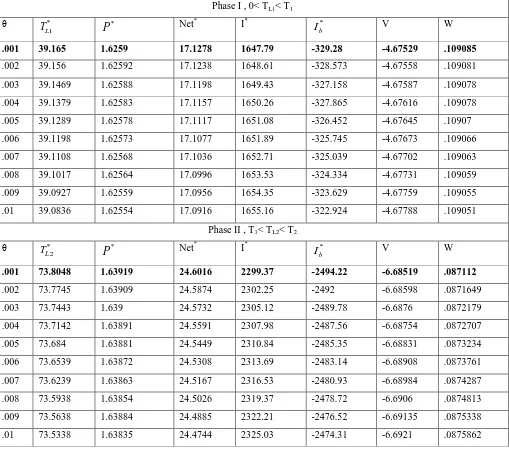
*, Net*, for the phase I and II are given in Table 1. Since the concavity of Net1 and Net2 with respect to TL is already proved in Theorem 1 (a) and

(b)thus we numerically check the concavity of Net with respect to P in the column ‗v‘ and joint concavity in column ‗W‘. In Table 2 numerical results are given for case 3. For Net3 condition for concavity of Net3 with respect to TL3 are presented under column ‗lhs‘ and ‗rhs‘. Joint concavity of Net are presented under column ‗W‘. From the table 1 and 2, the overall optimum value of the profit function is 24.6016

accomplish in Phase II atθ = .001 where

T

_L* = 73.8048,

P

*

= 1.63919, I* = 2299.37,

I

_b* = -2494.22, V = -6.68519 and W

[image:5.595.45.554.222.674.2]

= .087112

Table 1: Results of numerical example for Phase I and II Phase I , 0< TL1< T1

θ *

1

L

T

P

* Net* I*

I

b* V W

.001 39.165 1.6259 17.1278 1647.79 -329.28 -4.67529 .109085

.002 39.156 1.62592 17.1238 1648.61 -328.573 -4.67558 .109081

.003 39.1469 1.62588 17.1198 1649.43 -327.158 -4.67587 .109078

.004 39.1379 1.62583 17.1157 1650.26 -327.865 -4.67616 .109078

.005 39.1289 1.62578 17.1117 1651.08 -326.452 -4.67645 .10907

.006 39.1198 1.62573 17.1077 1651.89 -325.745 -4.67673 .109066

.007 39.1108 1.62568 17.1036 1652.71 -325.039 -4.67702 .109063

.008 39.1017 1.62564 17.0996 1653.53 -324.334 -4.67731 .109059

.009 39.0927 1.62559 17.0956 1654.35 -323.629 -4.67759 .109055

.01 39.0836 1.62554 17.0916 1655.16 -322.924 -4.67788 .109051

Phase II , T1< TL2< T2

θ *

2

L

T

_P

* Net* I*

I

_b* V W

.001 73.8048 1.63919 24.6016 2299.37 -2494.22 -6.68519 .087112

.002 73.7745 1.63909 24.5874 2302.25 -2492 -6.68598 .0871649

.003 73.7443 1.639 24.5732 2305.12 -2489.78 -6.6876 .0872179

.004 73.7142 1.63891 24.5591 2307.98 -2487.56 -6.68754 .0872707

.005 73.684 1.63881 24.5449 2310.84 -2485.35 -6.68831 .0873234

.006 73.6539 1.63872 24.5308 2313.69 -2483.14 -6.68908 .0873761

.007 73.6239 1.63863 24.5167 2316.53 -2480.93 -6.68984 .0874287

.008 73.5938 1.63854 24.5026 2319.37 -2478.72 -6.6906 .0874813

.009 73.5638 1.63884 24.4885 2322.21 -2476.52 -6.69135 .0875338

(6)

[image:6.595.43.561.65.276.2]

Table 2: Results of numerical example for Phase III

θ *

L

T

P

* Net* I*

I

b* lhs rhs W

.001 99.3265 1.63859 20.5895 1956.93 -4853.28 128.954 -.352305 .243925

.002 99.3576 1.63846 20.5639 1962.07 -4853.29 128.947 -.351906 .24401

.003 99.3887 1.63833 20.5384 1967.22 -4853.3 128.939 -.351508 .244096

.004 99.4198 1.63819 20.5128 1972.38 -4853.31 128.93 -.351107 .244182

.005 99.4509 1.63809 20.4872 1977.55 -4853.32 128.924 -.350718 .244353

.006 99.482 1.63793 20.4616 1982.72 -4853.33 128.915 -.350311 .244353

.007 99.531 1.6378 20.436 1987.91 -4853.34 128.907 -.349913 .244439

.008 99.5442 1.63766 20.4103 1993.1 -4853.35 128.898 -.349512 .244525

.009 99.5753 1.63753 20.3847 1998.3 -4853.36 128.89 -.349114 .24461

.01 99.6064 1.63739 20.359 2003.51 -4853.37 128.882 -.348713 .244696

lhs and rhs are the left hand side and right hand sight of expression (4)

Figure 2(a), 2(b) and 2(c) shows the joint concavity of the profit function Net1, Net2 and Net3 respectively with respect to TL1and P.

Figure 2(a):Joint concavity of Net1 with respect to

TL1and P.

F

igure 2(b): Joint concavity of Net2 with respect to

TL2and P

Figure 2(c): Joint concavity of Net3 with respect to

TL3and P.

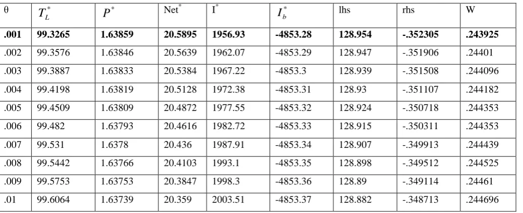
Now we solve Example 1 for the case when j = 0, that is the demand function is independent of price and linear in ‗t‘ to observe the change in optimal profit and the ordered inventory.

Example 2: All parameters of example 1 are same except j = 0

Result: From table 3 we observe that the maximum profit 34.7905 accomplish in Phase II at θ = .001 where

2

*

L

T = 64.5149,

P

* = 1.63919, I* = 4692.25,

I

_b* = -3785.12, V

[image:6.595.325.525.304.467.2] [image:6.595.53.274.340.664.2]

(7)

[image:7.595.131.468.59.707.2]

Table 3: Results of numerical example 2. Phase I, 0<

1

L

T < T1

θ *

1

L

T

P

* Net* I*

I

b*

.001 33.3671 1.6259 30.5976 3611.62 439.326

.002 33.3626 1.62592 30.5953 3612.06 439.89

.003 33.3583 1.62588 30.5916 3612.51 440.428

.004 33.3541 1.62583 30.5876 3612.96 440.954

.005 33.3498 1.62578 30.5837 3613.41 441.492

.006 33.3456 1.62573 30.5798 3613.86 442.017

.007 33.3413 1.62568 30.5759 3614.31 442.555

.008 33.337 1.62564 30.5722 3614.75 443.093

.009 33.3328 1.62559 30.5683 3615.2 443.618

.01 33.3285 1.62554 30.5443 3615.65 444.155

Phase II, T1< TL2< T2

.001 64.5149 1.63919 34.7905 4692.25 -3785.12

.002 64.5031 1.63909 34.7776 4675.32 -3783.38

.003 64.4913 1.639 34.7649 4677.11 -3781.63

.004 64.4794 1.63891 34.7522 4678.9 -3779.87

.005 64.4677 1.63881 34.7393 4680.69 -3778.14

.006 64.4558 1.63872 34.7266 4682.48 -3776.38

.007 64.444 1.63863 34.7139 4684.26 -3774.64

.008 64.4322 1.63854 34.7012 4686.05 -3772.9

.009 64.4184 1.63884 34.6968 4687.78 -3770.86

.01 64.4086 1.63835 34.6757 4689.61 -3769.41

Phase III, T2< TL3< T

.001 1.63859 99.7752 43.6012 4071.3 -64.8109

.002 1.63846 99.7898 43.5701 4076.27 -60.6112

.003 1.63833 99.8044 43.5391 4081.25 -56.4101

.004 1.63819 99.819 43.5077 4086.22 -52.2077

.005 1.63809 99.8337 43.4778 4091.21 -47.9752

.006 1.63793 99.8483 43.4455 4096.19 -43.7701

.007 1.6378 99.8629 43.4145 4101.18 -39.5638

.008 1.63766 99.8775 43.383 4106.17 -35.3561

.009 1.63753 99.8922 43.3519 4111.17 -31.1182

(8)

[image:8.595.40.516.65.274.2]

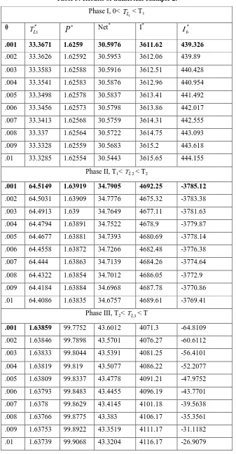
Table 5 Sensitivity analysis profit function

-100% -75% -50% -25% 0% 25% 50% 75% 100%

a 0.84135

3

0.631015 0.420677 0.210339 0 -0.210337 -0.420675 -0.631013 -0.84135

b 0.18988

9

0.142417 0.094944

8

0.047472

7

0 -0.0474714 -0.094944 -0.142416 -0.18989

j -1.13299 -0.76687

6

-0.462695 -0.209971 0 0.174452 0.319392 0.439813 0.53986

3

T

1

1.44966* 0.815444 0.362423

*

0.090606

9

0 0.0906095

*

0.362438

*

0.815493

*

1.44978*

P Not valid 1.98671 0.288849 0.036982

1

0 0.0156089 0.045615

8

0.078504

7

0.11041

8

V. SENSITIVITY ANALYSIS

In this section sensitivity analysis of the profit function with respect to decision variable and the demand parameters are presented. The sensitivity analysis of the optimal profit function which lies in phase 2 for θ = 0.001. In Table 3 contains the percent loss with respect to change in thedemand parameters (a, b and j) and the decision variables (T1, P). From Table 5 inference can be drawn that there is a linear change with respect to a and b but in opposite directions. For instance if we decreases ‗a‘ by 25 % then the percent loss will be 0.210339 while if we increase the ‗a‘ by 25 % then the percent loss will be -0.210337. It means that we

can

increase the profit by increasing the value of ‗a‘ it is due to by increasing ‗a‘ the demand rate increases. Similar type of change is observed with respect to ‗b‘ but with a different rate. Ifwe decreases ‗b‘ by 25% the percent loss will be0.0474727 while by increasing ‗b‘ by 25% the percent loss will be - 0.0474714

In case of ‗j‘ the profit function increases with the increment in ‗j‘ and decreases with the decrement in ‗j‘. The rate of change in profit function is more in case of negative change in ‗j‘ as compare to positive change in ‗j‘.

VI.CONCLUSION

We develop a mathematical model for trapezoidal type demand function which is price and time dependent, deterioration rate is time depended, shortage and partial backlogging allowed. Fruit vegetables and sea food ruin very fast so we adopted trapezoidal type demand function which may grow fast in first stage and reached on saturation point in second stage then get decline in last stage. We use numerical examples to analyzing profit function and applied sensitivity analysis to get change in profit as change in different parameters. We accomplished maximum profit in second stage.

REFERENCES

1. Ghare, P., and G. Schrader. "A model for exponentially decaying inventories." Journal of Industrial Engineering 15 (1963): 238-243.

2. Resh, Michael, Moshe Friedman, and Lineu C. Barbosa. "On a general solution of the deterministic lot size problem with time-proportional demand." Operations Research 24, no. 4 (1976): 718-725.

3. Donaldson, W. A. "Inventory replenishment policy for a linear trend in demand—an analytical solution." Journal of the operational research society 28, no. 3 (1977): 663-670.

4. Dave, Upendra, and L. K. Patel. "(T, S i) policy inventory model for deteriorating items with time proportional demand." Journal of the Operational Research Society 32, no. 2 (1981): 137-142.

5. Bose, S., A. Goswami, and K. S. Chaudhuri. "An EOQ model for deteriorating items with linear time-dependent demand rate and shortages under inflation and time discounting." Journal of the Operational Research Society 46, no. 6 (1995): 771-782.

6. Hariga, Moncer. "Optimal EOQ models for deteriorating items with time-varying demand." Journal of the Operational Research Society 47, no. 10 (1996): 1228-1246.

7. Hill, Roger M. "Inventory models for increasing demand followed by level demand." Journal of the Operational Research Society 46, no. 10 (1995): 1250-1259.

8. Mandal, B., and A. K. Pal. "Order level inventory system with ramp type demand rate for deteriorating items." Journal of interdisciplinary Mathematics 1, no. 1 (1998): 49-66.

9. Wu, Kun-Shan, and Liang-Yuh Ouyang. "A replenishment policy for deteriorating items with ramp type demand rate." Proceedings-National Science Council Republic of China Part a Physical Science and Engineering 24, no. 4 (2000): 279-286.

10. Skouri, Konstantaras, I. Konstantaras, Sotirios Papachristos, and Ioannis Ganas. "Inventory models with ramp type demand rate, partial backlogging and Weibull deterioration rate." European Journal of Operational Research 192, no. 1 (2009): 79-92.

11. Wu, Jong-Wuu, Chinho Lin, Bertram Tan, and Wen-Chuan Lee. "An EOQ inventory model with ramp type demand rate for items with Weibull deterioration." International Journal of Information and Management Sciences 10, no. 3 (1999): 41-51.

12. Manna, Swapan Kumar, and K. S. Chaudhuri. "An EOQ model with ramp type demand rate, time dependent deterioration rate, unit production cost and shortages." European Journal of Operational Research 171, no. 2 (2006): 557-566.

13. Giri, Bibhas Chandra, A. K. Jalan, and K. S. Chaudhuri. "Economic order quantity model with Weibull deterioration distribution, shortage and ramp-type demand." International Journal of Systems Science 34, no. 4 (2003): 237-243.

14. Wu, Kun-Shan. "An EOQ inventory model for items with Weibull distribution deterioration, ramp type demand rate and partial backlogging." Production Planning & Control 12, no. 8 (2001): 787-793.

15. Abad, P. L. "Optimal pricing and lot-sizing under conditions of perishability and partial backordering." Management science 42, no. 8 (1996): 1093-1104.

16. Deng, Peter Shaohua, Robert H-J. Lin, and Peter Chu. "A note on the inventory models for deteriorating items with ramp type demand rate." European Journal of Operational Research 178, no. 1 (2007): 112-120. 17. Cheng, Mingbao, and Guoqing

(9)

with trapezoidal type demand rate." Computers & Industrial Engineering 56, no. 4 (2009): 1296-1300.

18. Cheng, Mingbao, Bixi Zhang, and Guoqing Wang. "Optimal policy for deteriorating items with trapezoidal type demand and partial backlogging." Applied Mathematical Modelling 35, no. 7 (2011): 3552-3560.

19. Chuang, Kai-Wayne, Chien-Nan Lin, and Chun-Hsiung Lan. "Order policy analysis for deteriorating inventory model with trapezoidal type demand rate." Journal of networks 8, no. 8 (2013): 1838.

20. Zhao, Lianxia. "An inventory model under trapezoidal type demand, Weibull-distributed deterioration, and partial backlogging." Journal of Applied Mathematics 2014 (2014).

21. Dai, Zhuo, Faisal Aqlan, and Kuo Gao. "Optimizing multi-echelon inventory with three types of demand in supply chain." Transportation Research Part E: Logistics and Transportation Review 107 (2017): 141-177.

22. Pratibha Sharma, Ashish Sharma and Sanjay Jain ―Inventory model for deteriorating items with price and time-dependent seasonal demand” Int. J. Procurement Management, Vol. 12, No. 4, 2019

23. Hui-Ling Yang “An Inventory Model for Ramp-Type Demand with Two-Level Trade Credit Financing Linked to Order Quantity‖ Open Journal of Business and Management, 2019, 7, 427-446.

24. F.W. Harris, How many parts to make at once, (1913).

25. Wilson RH: A scientific routine for stock control. Harv Bus Rev 1934, 13: 116–128

26. Whitin, T.M., 1957 Theory of inventory management (Princeton University Press). You, S.P., 2005, Inventory policy for products with price and time-dependent demands, Journal of the Operational Research Society, 56, 870-873.

27. Wagner, Harvey M., and Thomson M. Whitin. "Dynamic version of the economic lot size model." Management science 5, no. 1 (1958): 89-96.

AUTHORSPROFILE

Jitendra Kaushik, Assistant Professor of Mathematics in the Department of MBA and PGDM at Sunstone Eduversity and Ph.D. Research scholar in Department of Mathematics, GLA University Mathura. He received degree of M.Phil in Mathematics from Bundelkhand University as merit holder. His research interest in Inventory modelling.