Abstract: The huge band variation in wind speed causes unpredictable swing in power generation and hence large divergence in system frequency leading to unpredictable situation for standalone applications. To overcome the above difficulties, WTG (wind turbine generator) is integrated with conventional thermal power system along with other distributed generation units such as FC (fuel cell), DEG (diesel engine generator), AE (aqua-electrolyser) and BESS (battery energy storage system) which form a hybrid power system. This paper concerns with automatic generation control (AGC) of an interconnected two area hybrid power system as mentioned above. Design and implementation of suitable controllers for AGC of above hybrid power system is a challenging job for operational and design engineers. Various control schemes proposed in this paper are conventional PID & PID controller with derivative filter (PIDF) and fuzzy-PID controller without (fuzzy-PID) and with derivative filter (fuzzy-PIDF) to achieve improved performance of AGC system in terms of frequency profile. The values of gain parameters of proposed controllers are designed using hybrid LUS-TLBO (Local Unimodal Sampling-Teaching Learning Based Optimization) algorithm. Superiority of fuzzy-PIDF controller over other proposed controllers are addressed. Robustness study of proposed fuzzy-PIDF controller is thoroughly demonstrated with change in system parameters and loading pattern. The work is further extended to analyze the transient phenomena of the AGC for a 3-area interconnected system having nonlinearities such as reheat turbine, governor dead band along with generation rate constraint for the thermal generating units.
Keywords: - Automatic Generation Control (AGC), Proportional-Integral-Derivative (PID), PID with derivative filter (PIDF), Local Unimodal Sampling (LUS), Teaching Learning Based Optimization (TLBO).
I. INTRODUCTION
With huge population and large industrial growth, the demand of electrical power is continuously growing in last few decades. Due to gradual reduction of fossil fuel and increase in cost of fuel, the desired demand of electrical power may not be compensated with traditional way power generation. Also the impact of global warming and harmful effect of emissions of carbon on surrounding due to thermal power generation using fossil fuel brings new ideas for clean and sustainable energy sources. In addition to that deregulation of electricity scenario worldwide develops new perspective for generation of low power which is known as distributed generation (DG). DG resources are generally used in the present scenario to fulfil the energy demand in the crisis. In the last decades technologies of DG system have
Revised Manuscript Received on August 05, 2019.
Bindod Kumar Sahu, Department of Electrical Engineering, ITER, SOA University, Bhubansewar, Odisha, India. [email protected].
* Pradeep Kumar Mohanty, Department of Electrical Engineering, ITER, SOA University, Bhubansewar, Odisha, India. [email protected].
provided solution to deficit in electrical energy to customers which are eco-friendly providing reliable and better power quality over conventional power generating possibility. The important issue in DG system is cost effective in terms of low transmission losses and less capital investments [1, 2]. A distributed generation system (DGs) is related with small electric power generating resources kept nearby its customers. The generating resources consists of wind energy, solar energy, diesel generator, biomass, fuel cells, geothermal power, energy storage system etc. Off grid electricity can be produced by using isolated power generating sources such as solar photo voltaic panels, micro-hydro plants, wind turbine generators (WTG) or fuel-power combustion engine generator set. Also a hybrid generating system can be implemented by combining two or more generating sources as stated above. Further to meet the hike of load demand of isolated consumer system, augmentation of DGs may be achieved by interconnecting it with traditional generating resources.
Now a day’s photo voltaic and wind energy are introduced as sources of renewable energy which are clean and predominantly available in nature. Also wind energy is emerging as competitive and leading renewable source due to gradual advancement in technology, low cost of components and hike in the cost of fossil fuels. Because of advanced research and development in semiconductor manufacturing technology, the capacity utilization of photo voltaic power generation is increasing rapidly in order to cope up the growing of electrical power demand. But energy conversion efficiency of photo voltaic generation is low and is costlier compared with wind power. However, unfortunately generation of both photo voltaic and wind power are highly changing in nature due to random variations in solar radiation and wind speed that leads to unreliable situation for standalone applications. Fuel cell (FC) also provides alternate resource of energy in the form of heat and electricity to its consumers. Taking the above view into account, photo voltaic generators and off shore wind turbine can be integrated with standby diesel engine generator (DEG), fuel cell (FC) and few energy storage devices like BESS (battery energy storage system), SMES (superconducting magnetic energy storage system), flywheel energy storage system (FESS), CAES (compressed air energy storage) which are generally considered to store the surplus amount of energy and supply during the peak load demand [3-5]. However, FESS is affected by low energy density and BESS suffers from the difficulties involved in low rate of discharge, reversal of power flow and maintenance. For low power (less than 100 kW) application of SMES is not
viable and it requires constant running of liquid helium
Design and implementation of Fuzzy-PID
Controller with Derivative Filter for AGC of
two-area interconnected Hybrid Power System
system. Further CAES suffers from low efficiency and unfavourable environmental impact. Another choice of storage is ultra-capacitor (UC)which is used to smoothen large and short time power solicitation of distributed generation system and meet the load demand on account of its fast response, flexible and modular structure [6, 7].
In fact isolated hybrid renewable energy system is often more complex unlike the system which is connected to grid. The variation in both velocity of wind and solar radiation results in unbalance between generated power and demanded load which causes alternation in system frequency and generated voltage from their base values. Such types of undue variation if permitted beyond certain tolerance limit may cause unpredicted system performance which in turn damages the connected equipment/devices. Therefore it is quite obvious to preserve the power balance in between generation and demand. Through governor action, system frequency is regulated called primary control and frequency can also be adjusted to its nominal value using load frequency control (LFC) known as secondary control [8]. The secondary control is considered to obtain specific frequency regulation and to
reduce tie-line unplanned power flows between
interconnected neighbouring areas. In case of normal running environment the frequency lies in a narrow band around the operating frequency value. But, during abnormal situation such as tripping of one or few large generating units, sudden hike in load demand or sudden loss of long tie-line between any two interconnected areas force to tackle the frequency control problem. Therefore, LFC issue need to be thoroughly studied to keep the system power balance, such that the frequency and tie-line power deviation remain within specified limits.
For satisfactory operation of hybrid system effective management, coordination and control action are required between the generating and energy storing elements. Previously, so many controllers are being presented to study the LFC problems for getting a suitable dynamic performance. The conventional controllers (constant gain) such as PID are generally employed due to their fastness, robustness and simplicity in operation and structure. Initially the gains were tuned basing upon past experience or approaching trial and error based method which were no longer remain appropriate in all the operating conditions. The simplest and oldest technique for determining the conventional PID controller gains is given in [9]. However this technique consumes more time for tuning and does not ensure the satisfactory performance of the process. Ziegler-Nichols [10] and Cohen-Coon [11] techniques are very popular and have been generally used for tuning the gains of controller. However the disadvantage of these techniques are (i) in case of noisy measurement, the performance of process may degrade and (ii) it makes the system’s response more oscillatory leading to increase in settling time due to too aggressive values of controller setting. Hence the controller gains obtained from classical methods need to be finely tuned using many recently developed soft computing techniques. Selection of proper controller and suitable optimization technique to optimally design the gain parameters in the field AGC have been attracting the researchers. Preedapong et al. [12] used linear matrix inequalities (LMI) method for
H
control design in order to achieve robustness against uncertainties. Olio et al. [13]discussed the theoretical approach and operational design of an advanced pluralistic LFC scheme. A new robust PID controller was designed for AGC of hydro-power system and presented in [14]. Kothari et al. [15] conferred discrete mode AGC for an interconnected reheat type thermal system employing a new area control error which is based on frequency deviation, deviation in tie-line power, time error and unplanned load variation. LFC for a realistic interconnected system within a restructuring competitive electricity market scenario is discussed in [16]. Bhongade et al. [17] illustrated the accomplishment of SMES (super conducting magnetic energy storage) unit of ANN based AGC of two area interconnected power system. SMES is employed to inject or absorb active power in the power system. Sudha and Santhi [18] proposed a type2 fuzzy logic based method for AGC of interconnected two area reheat type thermal power system with GRC. In [19] Mohanty et al. applied DE algorithm for optimally tuning the gain parameters of conventional I, PI and PID controllers for AGC of an interconnected two area multi-source power system. Sahu et al. [20] have employed hybrid DE-PSO algorithm for tuning the gain parameters of conventional and fuzzy based PID controller to solve the AGC issues in both two area and three area thermal system. Optimal design of fuzzy-PID controller using TLBO algorithm for AGC of a two area interconnected power system is discussed in [21]. Arya and Kumar [22] successfully presented fuzzy gain scheduling controllers optimized through Genetic Algorithm for both two-area non-reheat & reheat thermal power system and multi-source multi-area hydro thermal power system. Arya and Kumar [23]
demonstrated performance study of BFOA based
fuzzy-PI/fuzzy-PID controller of AGC for multi-area interconnected conventional/restructured electrical power system. Dominance of fractional-order fuzzy-PID (FOFPID) controller optimized through BFOA for AGC of interconnected power system is proved over fuzzy-PID and conventional PID controllers in [24].
In the present study a conventional power system along with an isolated DG system works within a local area and is no longer widely spread over vast geographical region. Further the unpredictability of irregular renewable resources with variation of generation increases the complexity of power system structure which leads to high fluctuation in frequency response and therefore the frequency stability issues becomes a challenging task for operational engineers. In [25] frequency control for a hybrid power system in an island is discussed. Small signal stability analysis for a hybrid energy storage system is presented by Lee and Wang [26]. PI controller based small signal stability analysis of hybrid DG system is discussed in [27]. Das et al. [28] considered GA based frequency controller for hybrid power system comprising of solar-thermal-diesel-wind energy system. In [29, 30] robust
H
controller for LFC in hybrid system is analyzed.In this paper a two-area interconnected hybrid power system is considered to study the AGC issues. Individual area of the power system model consists of a conventional reheat turbine type thermal generating unit along with distributed generating sources such as
WTG, FC, AE, DEG and BESS. Since wind power variation is
incorporation of DGs particularly power generation using wind turbines makes the power system more complicated thereby imposes new challenges in regards to power system control. The dynamic performance of conventional power plants differs from power system incorporated with wind power generation. Output power from wind power sources depends on geographical position, seasons and weather conditions. Due to change in weather, wind speed varies resulting deviation of generation of wind power from its forecast value which causes imbalance between generated power and load demand. In this study hybrid LUS-TLBO based conventional PID controller & PID controller with derivative filter (PIDF) and fuzzy PID controller & fuzzy PID controller with derivative filter (fuzzy-PIDF) are implemented to tackle the AGC issues in the proposed two area hybrid power system.
II. POWERSYSTEMUNDERSTUDY
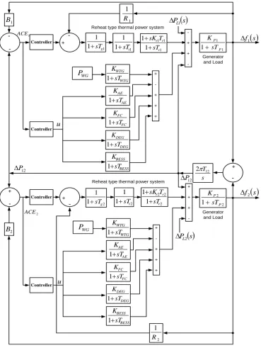
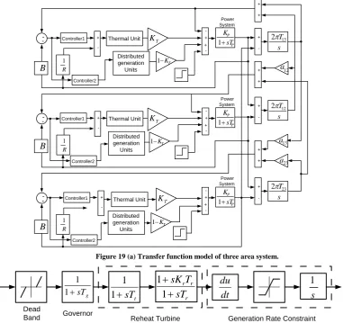
A two-area interconnected hybrid power system consisting of conventional reheat type thermal power generating unit along with various DGs is shown in Figure 1. Since AGC study mainly deals with small perturbations, linearized models of various generating units are taken into consideration to study the dynamic behaviour of the proposed hybrid power system. Transfer function model of different distributed generating units are presented as follows:
A. Wind Turbine Generator (WTG)
The output power generated by wind turbine generator mainly depends on the velocity of wind and the wind velocity continuously changes with respect to time. The output power (mechanical) of wind turbine
(
P
WT)
is directly proportional to cube of the wind speed as expressed below:3
2
1
W R P
WT
C
A
V
P
(1)Where
'
'
is air density of air in Kg/m3,'
C
P'
is thecoefficient of power,
'
A
R'
is swept area of blade measured in m2.'
V
W'
is the wind speed in m/sec. The expression of'
C
P'
is given by:
0
.
0184
(
3
)
3
.
0
15
)
3
(
sin
)
0167
.
0
44
.
0
(
P
C
(2) Where
'
'
is the tip speed ratio and'
'
is the pitch angle of the blade. Tip speed ratio'
'
is expressed as:W B B
V
w
R
(3)'
'
R
B is the radius of the blades in m,'
w
B'
is blade speed in rad/sec.The wind turbine generating system is extremely nonlinear in nature. The wind turbine mechanical output power varies when pitch controller is used to counteract the oscillations in grid frequency. According to wind speed, the pitch system adjusts the pitch angle suitably which in turn introduces nonlinearities. However for small perturbation the system nonlinearity may be linearized with some approximation. The
linearized transfer function of wind turbine generator is given by:
WTG WTG
WP WTG WTG
sT
K
P
P
T
1
(4)Where
K
WTG is the gain andT
WTG is the time constant of wind turbine generator.B. Aqua-Electrolyser (AE)
A part of the generation from WTG is fed to aqua-electrolyser for generation of hydrogen. When electric current is passed through aqueous electrolyte using electrodes, water is decomposed into hydrogen and oxygen. Hydrogen from AE is used by fuel cell which generates electrical power. Transfer function of AE is given by:
AE AE AE
AE
sT
K
u
P
T
1
(5)Where
K
AEis the gain andT
AEis the time constant of aqua-electrolyser.C. Fuel Cell (FC)
A fuel cell is primarily an electrochemical device that transforms chemical energy of hydrogen (fuel) into equivalent electrical energy by mixing air with gaseous hydrogen in the absence of combustion. A single fuel cell develops a very small voltage and to create sufficient voltage, fuel cells are arranged in series and parallel configurations which forms a fuel-cell stack. Various advantages of fuel cell generation in hybrid distributed power generating system are: high efficiency, low pollution, reusability of exhaust heat, diversity of fuels, and on-site installation. FC generating system is nonlinear possessing higher order. However for low frequency analysis, the system can be linearized to a first order system with transfer function expressed by:
FC FC FC
FC
sT
K
u
P
T
1
(6)Where
K
FCis the gain andT
FCis the time constant of fuel cell.D. Diesel Engine Generator (DEG)
Diesel engine acts as prime mover for the synchronous generator which generates electrical power. Due to uncertainty of wind power, imbalance between generated power and load demand occurs in a hybrid generating system. Since diesel engine generator has fast dynamic response and is capable of quickly rejecting the disturbance if any, it is the ultimate choice to maintain the balance between generated power and power demand. Due to presence of nonlinearity caused by the time delay in between injection and production of mechanical torque it is considered as nonlinear system. However with some approximation, the nonlinear DEG system can be linearized whose transfer function is expressed as:
DEG DEG DEG
DEG
sT
K
u
P
T
1
(7)Where
K
DEGis the gain andDEG
E. Battery Energy Storage System (BESS)
The variation of wind energy originates severe problems for suitable operation of power system. The possible solution is to use the energy storage devices such as BESS. BESS provides supplemental damping for power system swing which improves both dynamic and transient stability of the power system. BESS possesses characteristics of fast access time as well as large energy density. Therefore, BESS is effectual to store huge quantity of wind energy during peak generation from WTG.
BESS BESS BESS
BESS
sT
K
u
P
T
1
(8)Where
K
BESSandT
BESSare the gain and time constant of BESS respectively.In this study various controllers such as conventional PID without and with derivative filter & fuzzy-PID without and with derivative filter (fuzzy-PIDF) are employed to analyze the dynamic performance of proposed hybrid power system. Power frequency balancing is achieved by the help of control signals
'
u
1'
&'
u
2'
fed from the proposed design controller. In [29-30], the detailed mathematical model of various modules employed in hybrid DG power system are narrated and also data of various elements related with DG system under the study are mentioned. The equation given below describes the power balance in the system:L r DGS
e
P
P
P
P
(9)'
'
P
DGS represents power output from DG system,)
(
'
'
P
r
P
th represents the power output from reheat typethermal power system and
'
P
L'
is change in load demand and'
P
e'
represents the error produced in power supply. The total generated output power from hybrid DG system is given byBESS DEG
FC AE
WTG
DGS
P
P
P
P
P
P
(10) Where,
'
P
WTG'
,'
P
AE'
,'
P
FC'
,'
P
DEG'
and'
'
P
BESS represent the change in electrical power generated by WTG, AE, FC, DEG and BESS respectively. The influence of variation of wind power on the system frequency response is a major factor to analyze deeply the LFC issue in proposed hybrid system.The transfer function
'
T
st'
of the system is the ratio of frequency variation to variation in per unit value of error in power and is expressed as:P P
e st
sT
K
P
f
T
1
(11)Where,
'
T
P'
&'
K
P'
are equivalent time and gain constant of plant respectively. All the parameters of the proposed hybrid power system are given in Appendix.III. CONTROLSTRATEGY&IMPLEMENTATION OFHYBRIDLUS-TLBOALGORITHM
AGC issue in two area hybrid electrical power system shown in Figure 1 is studied by using various controllers like PID, PIDF, fuzzy PID and fuzzy PIDF. Structures of these controllers are shown in Figures 2-5. For the fuzzy logic based controllers structure of membership function is shown in Figure 6 and the rule base is depicted in Table 1. Triangular membership functions are employed for both the inputs and the output due to their simplicity and takes less computational time [31].
Any fuzzy logic system involves the following steps as depicted in Figure 7
• Fuzzyfication: - It is the process of conversion of crisp input into a linguistic variable with the help of membership functions.
• Interface engine: - It transforms the fuzzy input to fuzzy output by the help of if-then type fuzzy rules.
• Defuzzification: - It is the process of conversion of fuzzy output into crisp. There are many defuzzification processes; one of the most common methods is center of gravity technique.
Optimal gains of all these controllers are obtained by employing hybrid LUS-TLBO algorithm. A step load change of 0.01 pu for
P
L&
P
WTGis put in area-1 to study dynamic behavior of proposed hybrid power system. In this optimization process Integral Time Absolute Error (ITAE) is selected as objective function whose expression is given in equation (12). Controller gains are optimally designed by using hybrid LUS-TLBO algorithm by minimizing the fitness function. Controller gains are taken in the range [0.01-3.0] and range of derivative filter coefficient'
N
'
is taken [300-500]. Population dimension and maximum number of iterations are both taken as 100. Optimized value of various controllers’ gains are given in Table 2.dt
t
P
f
f
ITAE
tiet
t sim
).
(
20
1
(11)
Where
f
1 ,
f
2 &
P
tie represent the frequency deviations in area-1, area-2 & tie line power deviation respectively.'
t
sim'
indicates the simulation time.PID controller output in time domain and its transfer function are given by:
dt
t
de
K
dt
t
e
K
t
e
K
t
u
dt
i
p
0
(13)
s
K
s
K
K
s
E
s
U
TF
i dp
)
(
)
(
-Generator and Load
s f1
s PL1 1
1 R
+
-Generator and Load
sPL2
-+
+
12 P
12 P
1
B
2
B
-+
1
ACE
2
ACE
2 2
1 P
P
sT K
1 1
1 P
P
sT K
Controller
s f2 s T12
2
+ -+ + +
WG
P
WTG WTG
sT K
1
FC FC
sT K
1
AE AE
sT K
1
DEG DEG
sT K
1
BESS BESS
sT K
1
-+ +
-+ + +
-1 1 1
1 1
r r r
sT T sK
2 2 2 1 1
r r r
sT T sK
1
1 1
g
sT
1 1
1 t
sT
Controller
2 1
1
g
sT
1 2
1 t
sT
2 1 R
+ -+ + +
WG
P
WTG WTG
sT K
1
FC FC
sT K
1
AE AE
sT K
1
DEG DEG
sT K
1
BESS BESS
sT K
1
Controller
Controller
Reheat type thermal power system
Reheat type thermal power system
u
u
Figure 1 Proposed two area interconnected hybrid power system.
ti
dt
K
0
+
-)
(
t
r
e
(
t
)
+
+
u
(
t
)
+
-Disturbance
)
(
t
d
)
(
t
y
p
K
dt
d
K
d+
ReferenceInput
Error signal
PID Controller
Output
Plant
Plant Output
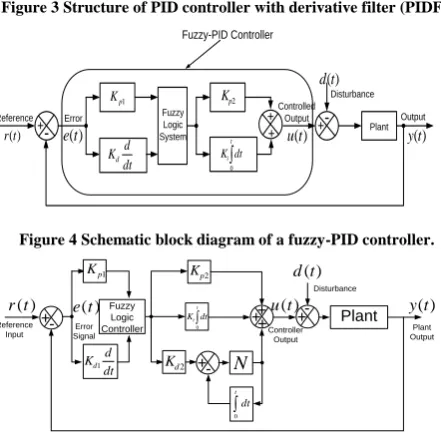
[image:5.595.116.486.54.556.2]PIDF controller’s transfer function is given by
s
N
Ns
K
s
K
K
TF
i dp
PIDF
(15)p
K
i
K
d
K
s
1
N
+-s
1
++ +
Proportional gain
Integral gain
Derivative gain
Filter Derivative filter
coefficient Integrator Error
Signal
[image:6.595.60.282.65.238.2]Controlled output
Figure 3 Structure of PID controller with derivative filter (PIDF).
+ -Disturbance
) (t d
Plant Output
) (t y
Controlled Output
) (t u
+
-) (t e
Error
dt d Kd
1
p
K
Fuzzy Logic System
t
idt
K 0
2
p
K
+ +
Fuzzy-PID Controller
Reference
[image:6.595.324.546.231.581.2]) (t r
Figure 4 Schematic block diagram of a fuzzy-PID controller.
) (t y
2
p
K
+-+++
+-tdt
0
+- Plant
Plant Output )
(t d
Disturbance
Controller Output
) (t u )
(t e
Error Signal ) (t r
Reference Input
N 2
d
K
t
idt K
0
Fuzzy Logic Controller
1
p
K
dt d Kd1
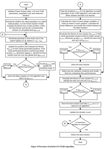
Figure 5 Fuzzy PID controller with derivative filter (fuzzy-PIDF).
PB PS
Z NS NB
1
0.5
0
[image:6.595.60.281.247.470.2]-1 -0.8 -0.4 0 0.4 0.8 1
Figure 6 Membership function for input and output.
Table 1 Rule base for fuzzy logic based controller.
ACE
ACE
NB NS Z PS PB
NB NB NB NB NS Z
NS NB NB NS Z PS
Z NB NS Z PS PB
PS NS Z PS PB PB
PB Z PS PB PB PB
Inputs Fuzzification Interface Engine
Fuzzy Rule Base
Defuzzification Outputs Inputs
Fuzzy Inputs
Fuzzy Outputs
(Crisp) (Crisp)
Figure 7 Block diagram representation of a fuzzy-logic system.
Overview of hybrid LUS-TLBO algorithm: - Local search algorithms are simple, more robust & gradient free and are applied widely in the area of hard computational problems. However main problem is that instead of the solution converges to global minima, there is a probability of convergence of the solution into a local minima. Also, as discussed previously global search techniques like PSO, DE, TLBO etc. are not preferred in case of a problem having less dimensions with few number of fitness evaluations or large dimensions with more fitness evaluations. So to get advantages of both local and global technique, LUS [32] algorithm is hybridized with TLBO [21] algorithm. Steps followed in LUS-TLBO algorithm are:
i. Initialization: - Generate initial population
'
x
k'
. LUS Algorithm begins hereii.Add
'
x
k'
with another vector'
a
k'
which is generated randomly in the sampling range'
r
'
to update the initial position.k k new
k
x
a
x
,
(16)iii. Compare fitness value of
'
x
k'
and'
x
k,new'
.iv. Accept
'
x
k,new'
if it is performing better else'
x
k'
and decrease the sampling range
'
r
'
. LUS Optimization algorithm ends here. TLBO Algorithm begins herev.Consider
'
x
k,new'
as first population.vi. Compute
'
M
diff'
which is the difference between mean results.
best tf d
diff
rand
x
T
M
M
(17)vii. Update
'
x
k,new'
by adding it with'
M
diff'
. diffnew k new
k
x
M
x
, 1
,
(18)viii. Accept
'
x
k,new1'
if performs better, else'
x
k,new'
. ix. Permit the learner for interaction with rest of thelearners to produce new solution
'
x
k,new2'
. x.Lastly select'
x
k,new1'
or'
x
k,new2'
as perperformance.
[image:6.595.74.257.488.604.2]Start
Initialize Power System data, LUS and TLBO parameters, population size and maximum
iteration
Randomly initialize the initial population (xi) called
initial position, run the Power System model, evaluate the fitness f(xi) of each position, select
the best fitness and set the corresponding solution as old global best (gbest,old)
Randomly generate a new vector (ai) in the
search space [-d, d], where d = xup - xlow
Update the position and evaluate the fitness f(xinew) of each newly generated positions. If the
newly generated position is performing better accept xi,new otherwise appept xi. Identify the best
solution and set it as new global best (gbest,new)
Is gbest,new
performing better? Accept
gbest,new
Yes Accept gbest,old and
update the sampling range ‘d’ No
Store the fittest solution of LUS algorithm and take it as gbest,new
A
A
Take the positions xi,new of LUS algorithm as initial
population of the TLBO algorithm, and select the fittest solution and take it as teacher
Calculate the mean of each design variables i.e. mean of marks in each subjects. Calculate the mean difference and modify the solution based on
the fittest solution
Evaluate the fitness of new solution f(xi,new1). If the
newly generated solution performs better accept xi,new1 otherwise accept xi,new. identify the best one
and set it as gbest,new1
B
Is gbest,new1
performing better? Accept
gbest,new1
Accept gbest,new
Select any two solutions randomly and modify them by comparing their performances
Evaluate the fitness of new solution f(xi,new2),
identify the best one and set it as gbest,new2
Is gbest,new2
performing better? Accept
gbest,new2
Accept gbest,new1
Is maximum iteration is reached?
Store the best solution and take xi.new2 as xi i.e.
input of LUS algorithm
Update the iteration count
Select the best solution
Stop
B
Yes
No
No Yes
Yes No
[image:7.595.82.522.55.680.2]Store the best solution
0 10 20 30 40 50 60 70 80 90 100 0.05
0.055 0.06 0.065 0.07 0.075 0.08 0.085 0.09
Generation
F
it
n
e
s
s
v
a
lu
e
[image:8.595.55.285.61.216.2]LUSTLBO TLBO LUS
Figure 9 Convergence characteristics of individual LUS& TLBO and hybrid LUS-TLBO algorithms.
IV. RESULT AND DISCUSSION
In this paper, AGC problem in a two area interconnected hybrid power system is addressed. Every area of the hybrid interconnected power system consists of a reheat type thermal generating unit and distributed generating units such as WTG, AE, FC, DEG and BESS. The proposed hybrid power system model as shown in Figure 1 is developed in MATLAB/Simulink environment and proposed hybrid LUS-TLBO program is written in .m file and taken to optimize the gains of proposed controllers whose values are depicted in Table 2. Using these controllers’ gains dynamic performance of the proposed two area hybrid power system is measured by applying a quick step load change of 0.01 pu in area-1. Figures 10-12 show the frequency alteration in area-1 (
f
1) & area-2 (
f
2) and tie-line power alteration (
P
tie) after undergoing a step load perturbation of 0.01 pu in area-1 with different proposed controllers. Overshoot (O
sh ), undershoot (U
sh) and settling time (T
s) (with 0.02% band for
f
1&
f
2 and 0.005% band for
P
tie) of
f
1,
f
2andtie
P
with various controllers, optimized through hybrid LUS-TLBO algorithm are depicted in Table 3.0 1 2 3 4 5 6 7 8 9 10
-14 -12 -10 -8 -6 -4 -2 0 2 4 6 8x 10
-3
Time in sec
f1
i
n
H
z
Fuzzy-PIDF Fuzzy-PID PIDF PID
Figure 10 Frequency deviation in area-1.
0 1 2 3 4 5 6 7 8 9 10
-6 -5 -4 -3 -2 -1 0 1 2 3x 10
-3
Time in sec
f2
i
n
H
z
Fuzzy-PIDF Fuzzy-PID PIDF PID
Figure 11 Frequency deviation in area-2.
0 1 2 3 4 5 6 7 8 9 10
-15 -10 -5 0
5x 10
-4
Time in sec
Ptie
i
n
p
u
[image:8.595.308.553.63.368.2]Fuzzy-PIDF Fuzzy-PID PIDF PID
Figure 12 Tie-line power deviation.
Four performance indices such as
U
sh,O
sh,T
sand the value of ITAE fitness function are chosen to compare the performance of various controllers. It is observed in Figures 10-12 and Table 3 that the suggested LUS-TLBO based fuzzy PIDF controller provides significant improvements in all the performance indices as against fuzzy-PID and conventional PID & PIDF controllers. Therefore, it can be concluded that the concept of adding derivative filter to fuzzy-PID controller improves the controller performance to a great extent. Percentage improvements inU
sh ,O
sh andT
s with LUS-TLBO based fuzzy PIDF controller as compared to LUS-TLBO based fuzzy PID and conventional PIDF & PID controllers are depicted in Table 4. Percentage improvements in the form of bar plot is shown in Figure 13 for better comparison of controllers’ performance.From Table 4 and Figure 13, it is noticed that proposed LUS-TLBO based fuzzy PIDF controller improves
U
shof1
f
,
f
2 &
P
tie by 65.61%, 71.01% & 66.88% respectively,O
sh of
f
1,
f
2&
P
tieby 57.12%, 65.29% & 62.44% andT
s of
f
1,
f
2&
P
tie by 36.33%, 67.97% and 73.24% respectively in comparison with LUS-TLBO based fuzzy PID controller. Similarly with the proposed fuzzy PIDF controller, improvement inU
sh of
f
1,
f
2&
P
tie are 78.82%, 90.29% and 87.99% respectively, inO
sh of
f
1,2
f
&
P
tie are 85.87%, 95.44% and 93.18% respectively, and inT
s of
f
1,
f
2 &
P
tie are 57.93%, 83.1% and 83.66% respectively in comparison with LUS-TLBO based PIDF controller. Also with the [image:8.595.49.287.520.662.2]improvement in
U
sh of
f
1 ,
f
2 &
P
tie are 83.55%, 93.33% and 90.85% respectively, inO
sh of
f
1 ,2
f
&
P
tie are 93.02%, 97.45% and 93.08% respectively [image:9.595.58.538.126.444.2]and in
T
s of
f
1,
f
2 &
P
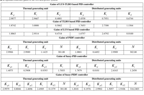
tie are 59.36%, 83.1% and 83.61% respectively in comparison with PID controller based on LUS-TLBO algorithm.Table 2 Optimal controller gains of the two area power system.
Gains of LUS-TLBO based PID controller
Thermal generating unit Distributed generating units
p
K
K
iK
dK
pK
iK
d2.9877 2.9667 0.4801 2.4558 0.7951 0.6744
Gains of TLBO based PID controller
1.8742 3.0000 0.5862 1.7653 2.7300 1.1564
Gains of LUS based PID controller
1.8863 2.9514 0.4718 1.6757 2.6792 0.0100
Gains of PIDF controller
Thermal generating unit Distributed generating units
p
K
K
iK
dN
K
pK
iK
dN
2.9906 2.9989 1.1425 301.00 1.0801 0.6492 2.9989 302.00
Gains of fuzzy-PID controller
Thermal generating unit Distributed generating units
1
p
K
K
dK
p2K
iK
p1K
dK
p2K
i1.4075 0.5908 0.9393 1.7055 1.7879 0.0101 2.6163 1.2450
Gains of fuzzy-PIDF controller
Thermal generating unit Distributed generating units
1
p
K
K
d1K
p2K
iK
d2N
K
p1K
d1K
p2K
iK
d2N
2.9979 0.8046 1.4696 2.4505 0.1379 301.00 1.2018 0.1976 2.9902 1.5057 1.9106 316.2403
Table 3
U
sh,O
shandT
s(0.02% band for
f
1&
f
2 and 0.005% band for
P
tie) of
f
1 ,
f
2 and
P
tie with different controllers.Table 4 Percentage improvement in
U
sh,O
shandT
swith LUS-TLBO based PIDF controller. Controller1
f
f
2
P
tieITAE
sh
U
in Hz
310
sh
O
in Hz
310
s
T
in sec
sh
U
in Hz
310
sh
O
in Hz
310
s
T
in sec
sh
U
in pu
310
sh
O
in pu
310
s
T
in sec
LUS-TLBO fuzzy-PIDF -2.0602 0.4541 1.91 -0.3515 0.0721 0.98 -0.1368 0.0296 1.18 0.0043
LUS-TLBO fuzzy-PID -5.9906 1.0590 3.00 -1.2123 0.2077 3.06 -0.4130 0.0788 4.41 0.0121
LUS-TLBO PIDF -9.7276 3.2142 4.54 -3.6202 1.58 5.8 -1.1392 0.4341 7.22 0.0692
LUS-TLBO PID -12.5274 6.5090 4.70 -5.2733 2.8286 5.80 -1.4944 0.4277 7.20 0.0513
TLBO-PID -13.0448 8.1029 5.47 -5.9968 4.7565 5.55 -1.7406 0.8149 6.67 0.0624
LUS-PID -13.7321 9.3202 5.61 -6.4682 5.6245 5.35 -1.8446 0.9120 6.83 0.0647
1
f
f
2
P
tieITAE
sh
U
O
shT
sU
shO
shT
sU
shO
shT
sIn comparison with LUS-TLBO based fuzzy-PID controller
65.61 57.12 36.33 71.01 65.29 67.97 66.88 62.44 73.24 64.46
In comparison with LUS-TLBO based PIDF controller
78.82 85.87 57.93 90.29 95.44 83.10 87.99 93.18 83.66 93.79
In comparison with LUS-TLBO based PID controller
1
f of Ush
f2
of Ush
tie
sh P of U
1
f of Osh
f2
of Osh
tie
sh P of O
1
f of Ts
f2
of Ts
tie
s P
of T
ITAE
1 2 3 4 5 6 7 8 9 10
0 10 20 30 40 50 60 70 80 90 100
P
e
rc
e
n
ta
g
e
I
m
p
ro
v
e
m
e
n
t
[image:10.595.306.548.73.511.2]In comparison with fuzzy-PID In comparison with PIDF In comparison with PID
Figure 13 Percentage improvement in the form of bar plot.
Integral time absolute error (ITAE) also plays a main role in optimally designing the values of controller gains. Less is the ITAE value better is the system performance and vice versa. It is seen in Table 4 and Figure 13 that improvement in ITAE with proposed LUS-TLBO based fuzzy PIDF controller are 64.46%, 93.79% and 91.62% in comparison with LUS-TLBO based fuzzy-PID and conventional PIDF & PID controller respectively. Therefore it can be finally concluded that the proposed LUS-TLBO based fuzzy PIDF controller outperforms the other proposed controllers.
V. SENSITIVITYANALYSIS
Sensitive/robustness analysis of the proposed LUS-TLBO based fuzzy PIDF controller is done in order to prove its efficacy under system parametric variation. With optimal controller gains as depicted in Table 2, robustness analysis is done by (i) randomly varying the loading pattern in both the areas of the power system and (ii) varying one at a time, parameters of the hybrid power system in the range of -50% to +50% in steps of 25% of their nominal values.
A. Sensitivity analysis by randomly varying the loading patterns
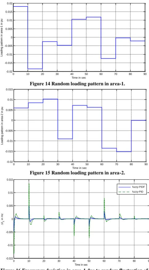
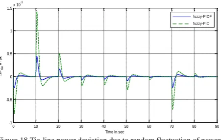
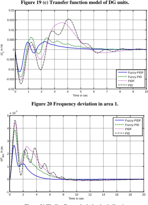
To prove the robustness of the suggested controller against variation in electrical power demand, both the area of the power system subjected to randomly varying loading pattern as shown in Figures 14 and 15 respectively. This study is done by taking the nominal system parameters as given in Appendix. Frequency deviation in area 1 & area 2 and tie-line power deviation due to randomly varying loading patterns in area 1 (Figure 14) and area 2 (Figure 15) are shown in Figures 16, 17 and 18 respectively. It is noted from Figures 16, 17 and 18 that both fuzzy-PIDF and fuzzy-PID controllers’ exhibit stable dynamic performance under randomly varying loading patterns in area-1 and area-2. However fuzzy-PIDF controller exhibits less undershoot/overshoot and settles quickly as against fuzzy PID controller. Therefore, finally it can be inferred that the proposed LUS-TLBO optimized fuzzy-PIDF controlled AGC system for the hybrid power system is robust against variation in loading conditions.
0 10 20 30 40 50 60 70 80 90
-0.02 -0.015 -0.01 -0.005 0 0.005 0.01 0.015 0.02
Time in sec
L
o
a
d
in
g
p
a
tt
e
rn
i
n
a
re
a
-1
i
n
p
u
Figure 14 Random loading pattern in area-1.
0 10 20 30 40 50 60 70 80 90
-0.02 -0.015 -0.01 -0.005 0 0.005 0.01 0.015
Time in sec
L
o
a
d
in
g
p
a
tt
e
rn
i
n
a
re
a
-2
i
n
p
u
Figure 15 Random loading pattern in area-2.
0 10 20 30 40 50 60 70 80 90
-0.015 -0.01 -0.005 0 0.005 0.01 0.015
Time in sec
f1
i
n
H
z
fuzzy-PIDF
fuzzy-PID
Figure 16 Frequency deviation in area-1 due to random fluctuation of power demand in area-1 and area-2.
0 10 20 30 40 50 60 70 80 90
-8 -6 -4 -2 0 2 4 6 8
10x 10
-3
Time in sec
2
i
n
H
z
fuzzy-PIDF
[image:10.595.53.286.111.263.2]fuzzy-PID
[image:10.595.307.552.519.681.2]0 10 20 30 40 50 60 70 80 90 -1
-0.5 0 0.5 1 1.5x 10
-3
Time in sec
Pti
e
i
n
p
u
fuzzy-PIDF
[image:11.595.57.283.51.194.2]fuzzy-PID
Figure 18 Tie-line power deviation due to random fluctuation of power demand in area-1 and area-2.
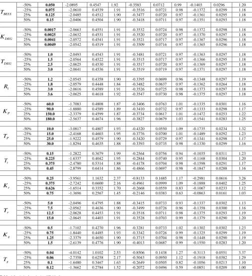
B. Sensitivity analysis by varying all the parameters of the proposed power system
In this study, all the system parameters are varied within -50% to 50% in steps of 25% to prove the robustness of the suggested LUS-TLBO based fuzzy PIDF controller against parametric variation. A step load change of 1% is taken in area 1 in this study and
U
sh ,O
sh &T
s of
f
1 ,2
f
&
P
tieare depicted in Table 5. Statistical study of Table 5 is carried out by taking maximum, minimum & mean value along with standard deviation which are mentioned in Table 6. In Table 6, it is clearly verified that every transient parameter such asU
sh,O
sh&T
schange within a narrow range. Percentage deviation of mean values ofU
sh ,sh
O
&T
sfrom their nominal values are given in Table 7. It is seen from Table 7 that with system parametric variation the percentage deviation of mean values from nominal value lie in the range of -6.01 to 0.77 % only.From above Tables, Figures and analysis it is concluded that overshoot, undershoot and settling time of
2
1
,
f
f
and
P
tie of the suggested two area hybrid power system with LUS-TLBO based fuzzy PIDF controller vary within acceptable range. Hence, it can be conferred that the proposed LUS-TLBO based fuzzy PIDF controller is robust against variation in loading pattern as well as parametric variation.Table 5 Robustness analysis with parametric variation using the proposed LUS-TLBO optimized fuzzy-PIDF controller.
Paramet ers
% age deviation
Numerical values
after deviation
3
10
sh
U
of
f
1 (in Hz)3
10
sh
O
of
f
1 (in Hz)s
T
of
1
f
(in sec)3
10
sh
U
of
f
2 (in Hz)3
10
sh
O
of
f
2 (in Hz)s
T
of
2
f
(in sec)3
10
sh
U
of
tie
P
(in pu)3
10
sh
O
of
tie
P
(in pu)s
T
of
tie
P
(in sec)WTG
K
-50% 0.5 -2.1281 0.3029 1.77 -0.3796 0.0369 1.15 -0.1499 0.0152 1.44 -25% 0.75 -2.0941 0.3766 1.84 -0.3571 0.0522 1.05 -0.1429 0.0215 1.30 25% 1.25 -2.0313 0.5377 1.97 -0.3343 0.0953 0.90 -0.1306 0.0393 1.08 50% 1.5 -2.0026 0.6229 2.02 -0.3170 0.1216 0.84 -0.1247 0.0502 2.53
WTG
T
-50% 0.75 -1.9506 0.5165 1.64 -0.3027 0.0663 0.79 -0.1179 0.0266 0.97 -25% 1.125 -2.0231 0.4863 1.82 -0.3298 0.0713 0.90 -0.1295 0.0291 1.09 25% 1.875 -2.0867 0.4272 1.96 -0.3513 0.0712 1.02 -0.1411 0.0295 1.25 50% 2.25 -2.1045 0.4011 1.98 -0.3627 0.0695 1.06 -0.1446 0.0289 1.30
AE
K
-50% 0.001 -2.0846 0.4553 1.91 -0.3531 0.0721 0.98 -0.1381 0.0297 1.19 -25% 0.0015 -2.0667 0.4535 1.91 -0.3532 0.0720 0.98 -0.1372 0.0297 1.18 25% 0.0025 -2.0538 0.4520 1.91 -0.3498 0.0719 0.97 -0.1365 0.0297 1.18 50% 0.003 -2.0475 0.4513 1.91 -0.3472 0.0720 0.97 -0.1362 0.0296 1.18
AE
T
-50% 0.25 -2.0422 0.4526 1.91 -0.3485 0.0719 0.97 -0.1362 0.0295 1.18 -25% 0.375 -2.0534 0.4556 1.91 -0.3489 0.0719 0.97 -0.1365 0.0297 1.18 25% 0.625 -2.0647 0.4544 1.91 -0.3528 0.0720 0.98 -0.1370 0.0297 1.18 50% 0.75 -2.0669 0.4531 1.91 -0.3525 0.0720 0.98 -0.1372 0.0297 1.18
FC
K
-50% 0.005 -2.0685 0.4553 1.91 -0.3530 0.0724 0.98 -0.1374 0.0297 1.18 -25% 0.0075 -2.0649 0.4538 1.91 -0.3527 0.0720 0.97 -0.1371 0.0297 1.18 25% 0.0125 -2.0555 0.4519 1.91 -0.3513 0.0717 0.97 -0.1366 0.0296 1.18 50% 0.015 -2.0509 0.4526 1.91 -0.3491 0.0720 0.97 -0.1363 0.0296 1.18
FC
T
-50% 2.0 -2.0426 0.4533 1.91 -0.3459 0.0721 0.97 -0.1359 0.0297 1.18 -25% 3.0 -2.0542 0.4518 1.91 -0.3509 0.0717 0.97 -0.1365 0.0296 1.18 25% 5.0 -2.0639 0.4533 1.91 -0.3522 0.0720 0.97 -0.1370 0.0297 1.18 50% 6.0 -2.0664 0.4543 1.91 -0.3532 0.0721 0.98 -0.1372 0.0297 1.18
BESS
K
[image:11.595.47.558.322.813.2]BESS
T
-50% 0.050 -2.0895 0.4547 1.92 -0.3583 0.0712 0.99 -0.1403 0.0296 1.20 -25% 0.075 -2.0610 0.4539 1.91 -0.3516 0.0721 0.98 -0.1372 0.0299 1.18 25% 0.125 -2.0485 0.4512 1.90 -0.3477 0.0720 0.97 -0.1361 0.0295 1.18 50% 0.15 -2.0406 0.4504 1.90 -0.3418 0.0711 0.97 -0.1351 0.0293 1.18
DEG
K
-50% 0.0017 -2.0663 0.4551 1.91 -0.3532 0.0724 0.98 -0.1372 0.0298 1.18 -25% 0.0025 -2.0632 0.4531 1.91 -0.3520 0.0720 0.97 -0.1370 0.0297 1.18 25% 0.0041 -2.0572 0.4541 1.91 -0.3521 0.0717 0.97 -0.1367 0.0296 1.18 50% 0.0049 -2.0542 0.4519 1.91 -0.3509 0.0716 0.97 -0.1365 0.0296 1.18
DEG
T
-50% 1.0 -2.0493 0.4543 1.91 -0.3481 0.0721 0.97 -0.1363 0.0297 1.18 -25% 1.5 -2.0564 0.4522 1.91 -0.3515 0.0717 0.97 -0.1366 0.0295 1.18 25% 2.5 -2.0625 0.4530 1.91 -0.3517 0.0720 0.97 -0.1369 0.0297 1.18 50% 3.0 -2.0641 0.4536 1.91 -0.3519 0.0719 0.97 -0.1371 0.0297 1.18
1
R
-50% 1.2 -2.0545 0.4358 1.90 -0.3395 0.0699 0.96 -0.1348 0.0297 1.19 -25% 1.8 -2.0579 0.4448 1.84 -0.3482 0.0637 0.97 -0.1362 0.0264 1.18 25% 3.0 -2.0616 0.4589 1.91 -0.3526 0.0725 0.98 -0.1373 0.0297 1.18 50% 3.6 -2.0625 0.4618 1.92 -0.3547 0.0730 0.98 -0.1375 0.0297 1.18
P
K
-50% 60.0 -1.7083 0.4808 1.87 -0.3406 0.0763 1.01 -0.1335 0.0301 1.16 -25% 90.0 -1.8880 0.4589 1.89 -0.3410 0.0732 0.97 -0.1333 0.0298 1.17 25% 150.0 -2.3379 0.4599 1.87 -0.3734 0.0617 1.01 -0.1472 0.0253 1.22 50% 180.0 -2.5637 0.4674 1.96 -0.3827 0.0679 1.03 -0.1541 0.0283 1.25
P
T
-50% 10.0 -3.0817 0.4807 1.93 -0.4320 0.0550 1.09 -0.1735 0.0234 1.32 -25% 15.0 -2.4168 0.4603 1.95 -0.3776 0.0700 1.01 -0.1489 0.0292 1.23 25% 25.0 -1.9222 0.4579 1.90 -0.3420 0.0729 0.97 -0.1341 0.0298 1.17 50% 30.0 -1.8294 0.4635 1.88 -0.3393 0.0735 0.98 -0.1330 0.0299 1.16
t
T
-50% 0.15 -1.2822 0.3679 1.99 -0.2564 0.0756 0.94 -0.1035 0.0311 1.23 -25% 0.225 -1.6337 0.4042 1.95 -0.2844 0.0740 0.95 -0.1168 0.0304 1.20 25% 0.375 -2.4780 0.5314 1.88 -0.4178 0.0704 0.98 -0.1598 0.0291 1.17 50% 0.45 -2.8799 0.6414 1.86 -0.4866 0.0697 0.98 -0.1847 0.0288 1.16
r
K
-50% 0.25 -3.9561 1.1632 2.37 -0.8133 0.1685 1.17 -0.2981 0.0616 3.26 -25% 0.375 -2.7242 0.6600 2.16 -0.4961 0.0999 1.09 -0.1888 0.0402 1.25 25% 0.626 -1.6514 0.3352 1.70 -0.2668 0.0559 0.83 -0.1067 0.0233 1.12 50% 0.75 -1.3696 0.2567 1.45 -0.2146 0.0383 0.63 -0.0863 0.0161 1.03
r
T
-50% 5.0 -2.0496 0.4795 1.88 -0.3415 0.0733 0.93 -0.1337 0.0302 1.13 -25% 7.5 -2.0562 0.4636 1.90 -0.3499 0.0726 0.96 -0.1358 0.0300 1.16 25% 12.5 -2.0628 0.4453 1.91 -0.3518 0.0711 0.98 -0.1375 0.0293 1.19 50% 15.0 -2.0645 0.4403 1.91 -0.3528 0.0703 0.99 -0.1379 0.0290 1.20
g K
-50% 0.5 -1.7102 0.4270 1.96 -0.3281 0.0733 1.02 -0.1302 0.0302 1.23 -25% 0.75 -1.8440 0.4485 1.93 -0.3342 0.0726 0.99 -0.1325 0.0299 1.19 25% 1.25 -2.3379 0.4650 1.90 -0.3715 0.0704 0.98 -0.1448 0.0290 1.19 50% 1.5 -2.6139 0.4776 1.90 -0.4013 0.0687 0.99 -0.1550 0.0283 1.20
g
T
[image:12.595.48.555.46.601.2]-50% 0.04 -4.0142 1.0102 2.53 -0.8506 0.1438 1.27 -0.3113 0.0551 3.37 -25% 0.06 -2.7358 0.6258 2.17 -0.5043 0.0950 1.12 -0.1918 0.0382 1.29 25% 0.1 -1.6480 0.3467 1.63 -0.2649 0.0505 0.82 -0.1056 0.0213 1.10 50% 0.12 -1.3662 0.2784 1.52 -0.2072 0.0496 0.59 -0.0851 0.0209 1.00
Table 6 Statistical analysis of Table 5.
Statistical parameters
1
f
f
2
P
tiesh
U (in
Hz)
)
10
(
3sh
O (in
Hz)
)
10
(
3s
T
(in sec)
sh
U (in
Hz)
)
10
(
3sh
O (in
Hz)
)
10
(
3s
T
(in sec)
sh
U (in
pu)
)
10
(
3sh
O (in
Hz)
)
10
(
3s
T
(in sec)
Maximum
value -4.0142 1.1632 2.53 -0.8506 0.1685 1.27 -0.3113 0.0616 3.37
Minimum
value -1.2822 0.2567 1.45 -0.2072 0.0369 0.59 -0.0851 0.0152 0.97
Average
value -2.1217 0.4719 1.9083 -0.3634 0.0733 0.9725 -0.1418 0.0300 1.2615 Standard